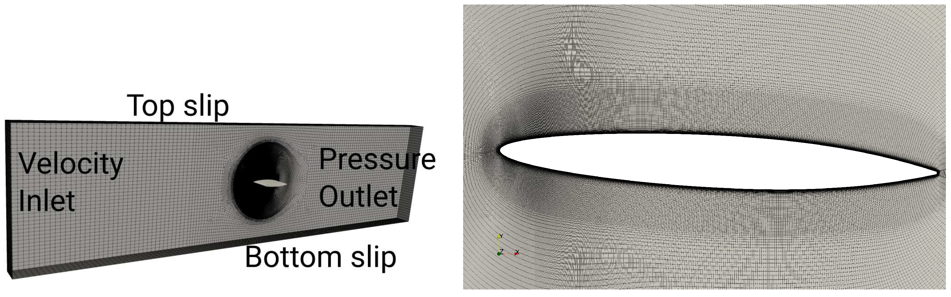
Figure 1.
Simulation domain (left) and closer view of computational grids (right).
Figure 1.
Simulation domain (left) and closer view of computational grids (right).
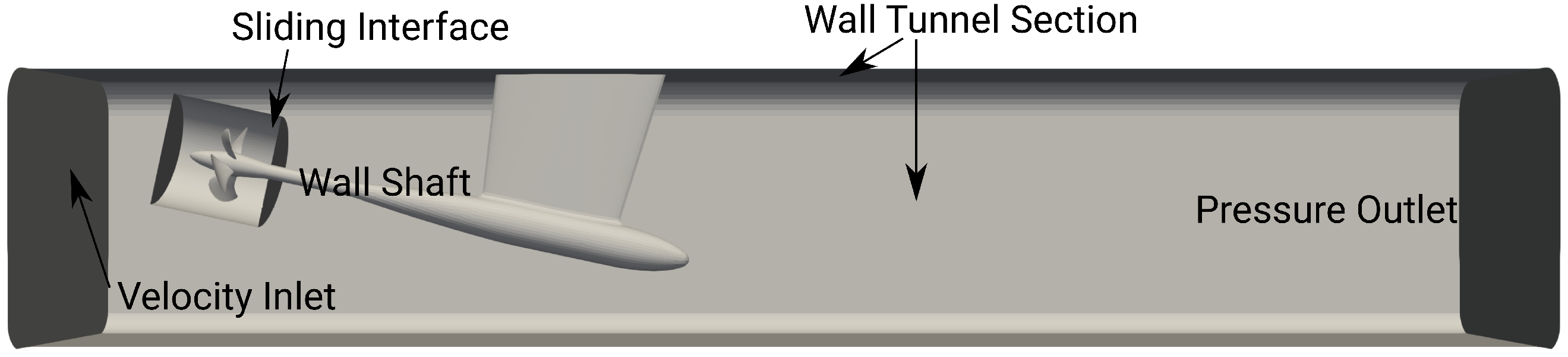
Figure 2.
Simulation domain and boundary conditions.
Figure 2.
Simulation domain and boundary conditions.
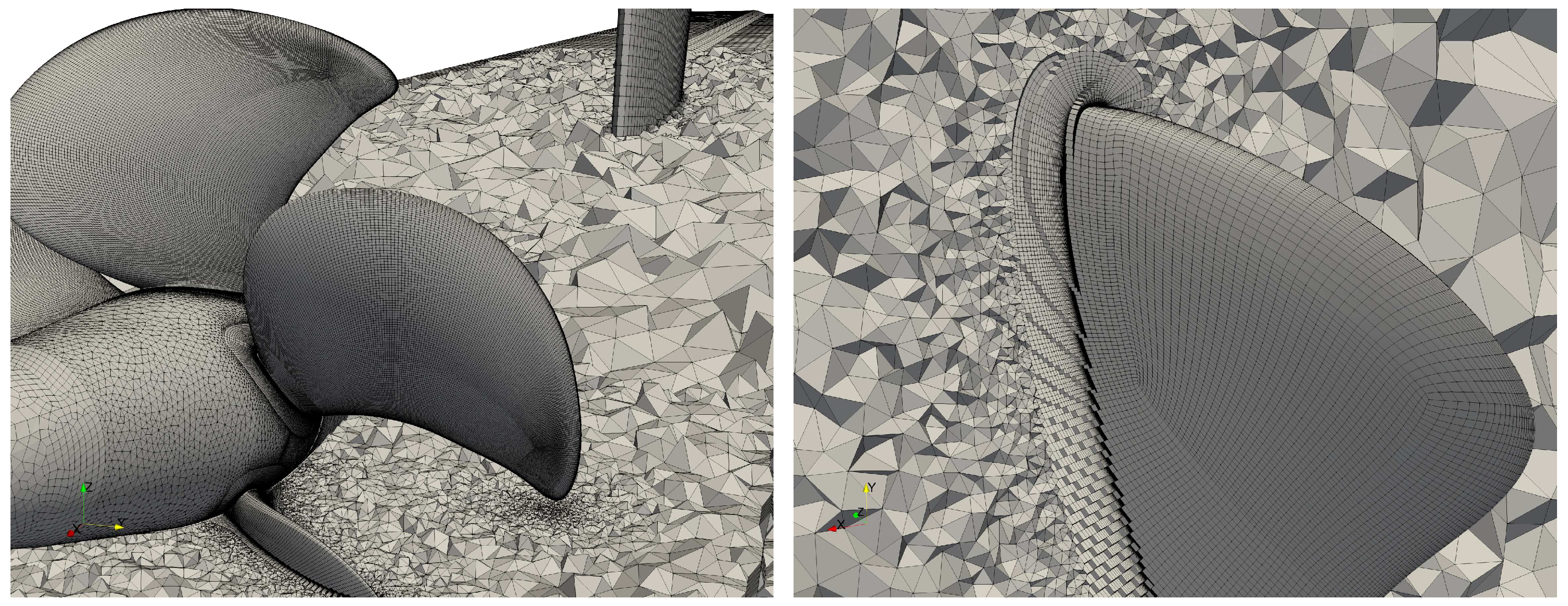
Figure 3.
Close-up view at the blade surface mesh and tip volume grids.
Figure 3.
Close-up view at the blade surface mesh and tip volume grids.
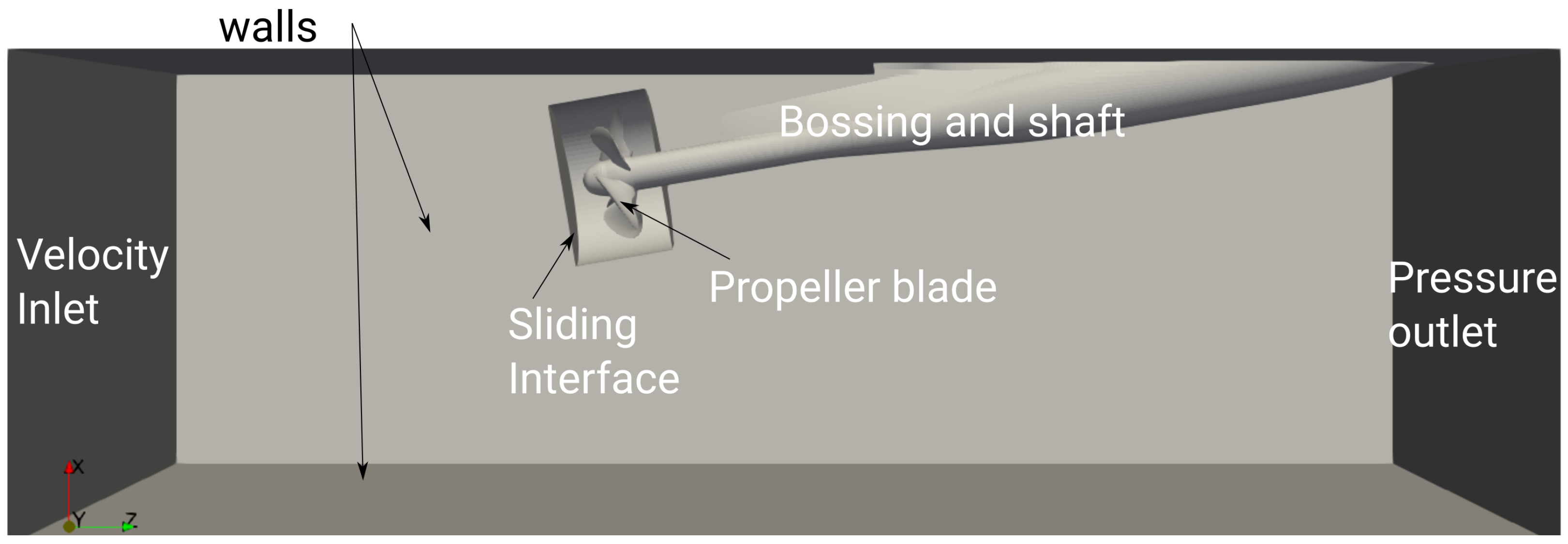
Figure 4.
Simulation configuration for propeller A tested in the cavitation tunnel.
Figure 4.
Simulation configuration for propeller A tested in the cavitation tunnel.
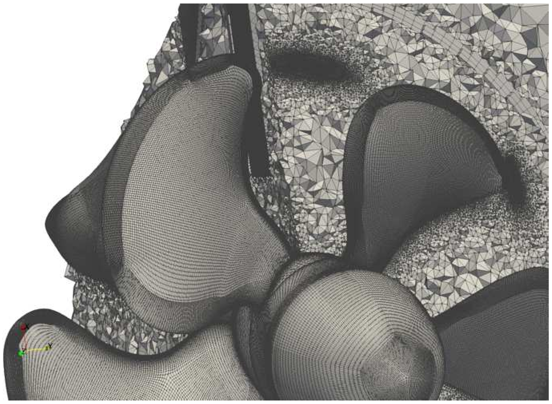
Figure 5.
Closer view of surface and volume mesh close to the propeller blades.
Figure 5.
Closer view of surface and volume mesh close to the propeller blades.
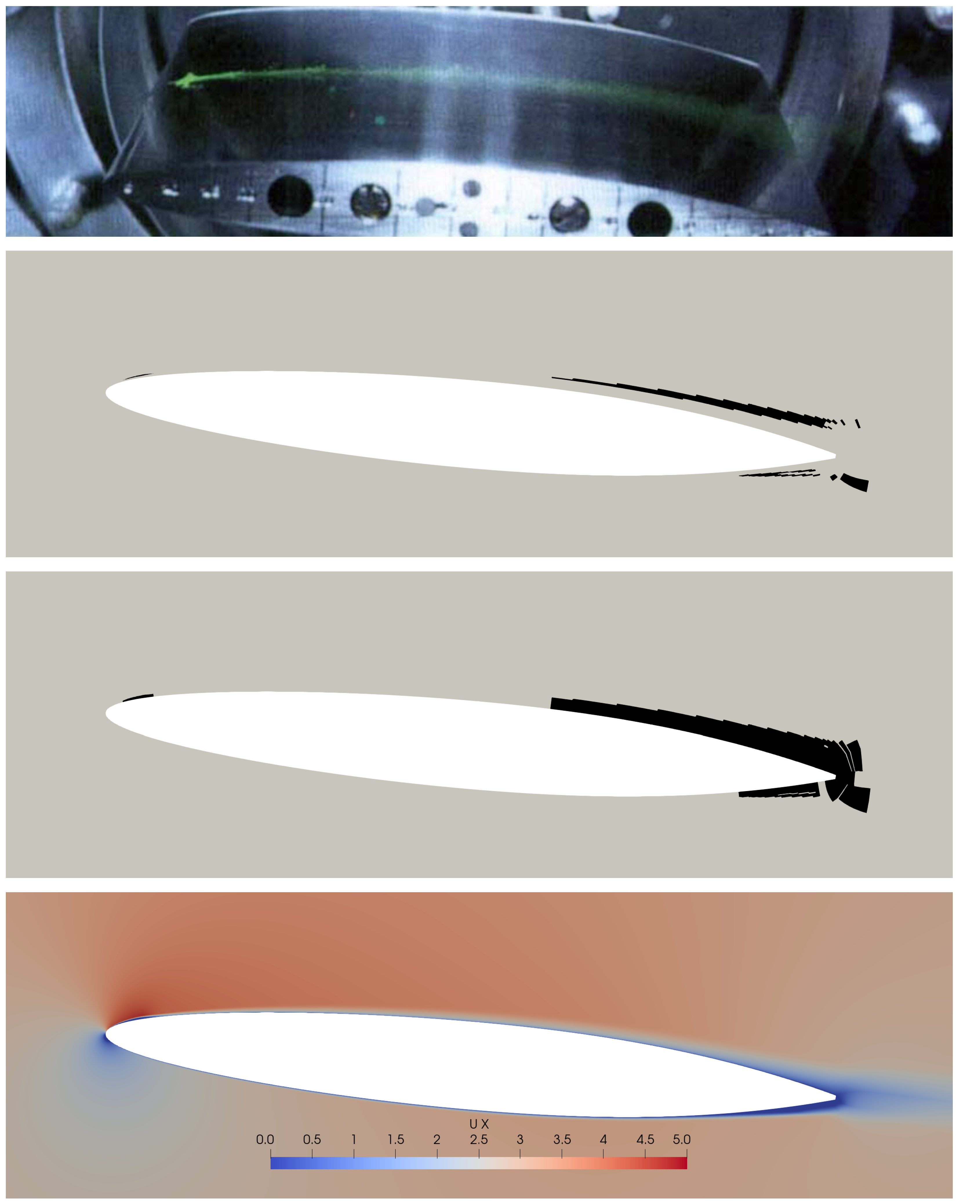
Figure 6.
Visualization of laminar transition for NACA16012, AoA = , Re = 300,000. From top to bottom: experimental photograph; predicted ; predicted ; predicted velocity in flow direction.
Figure 6.
Visualization of laminar transition for NACA16012, AoA = , Re = 300,000. From top to bottom: experimental photograph; predicted ; predicted ; predicted velocity in flow direction.
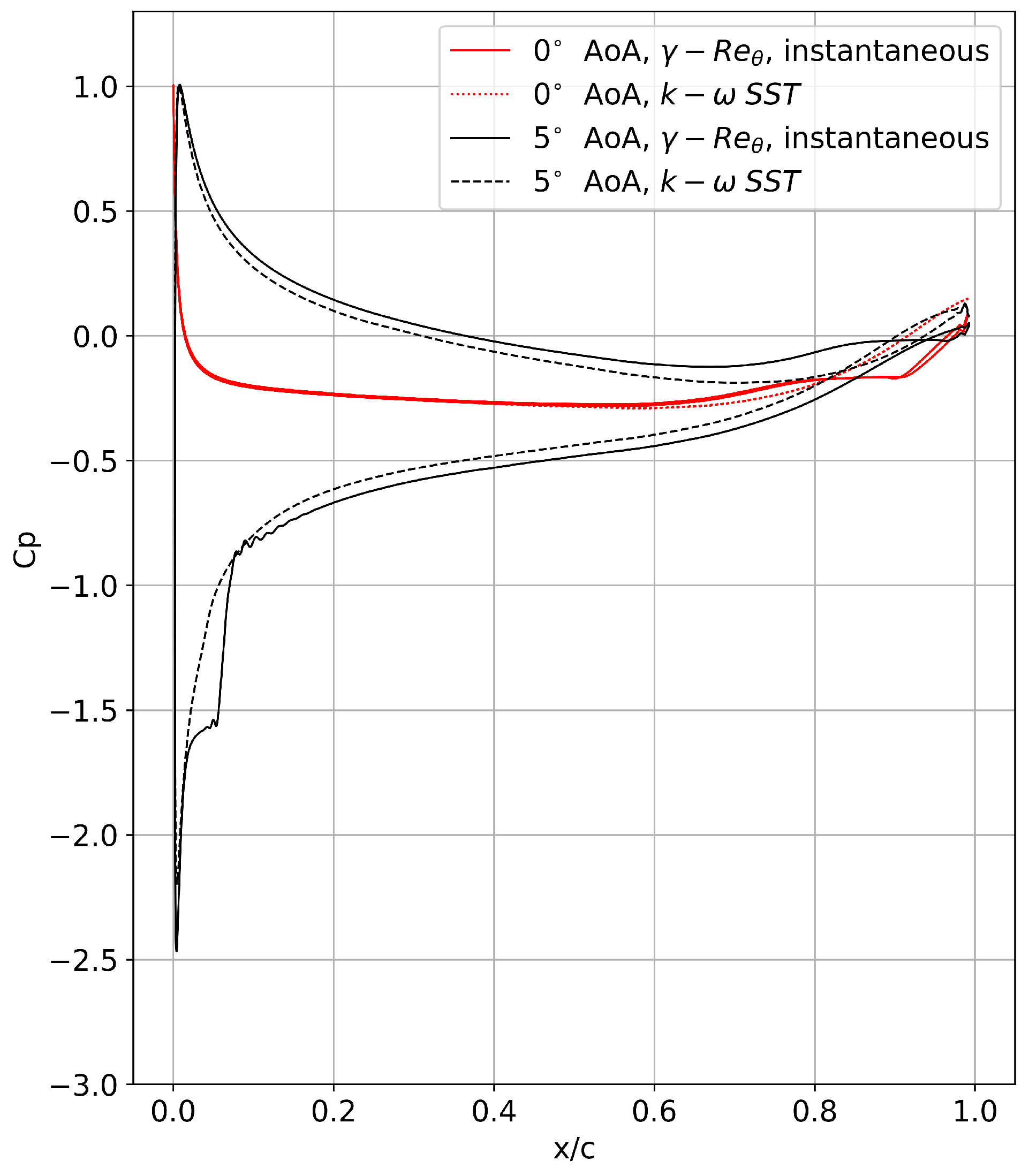
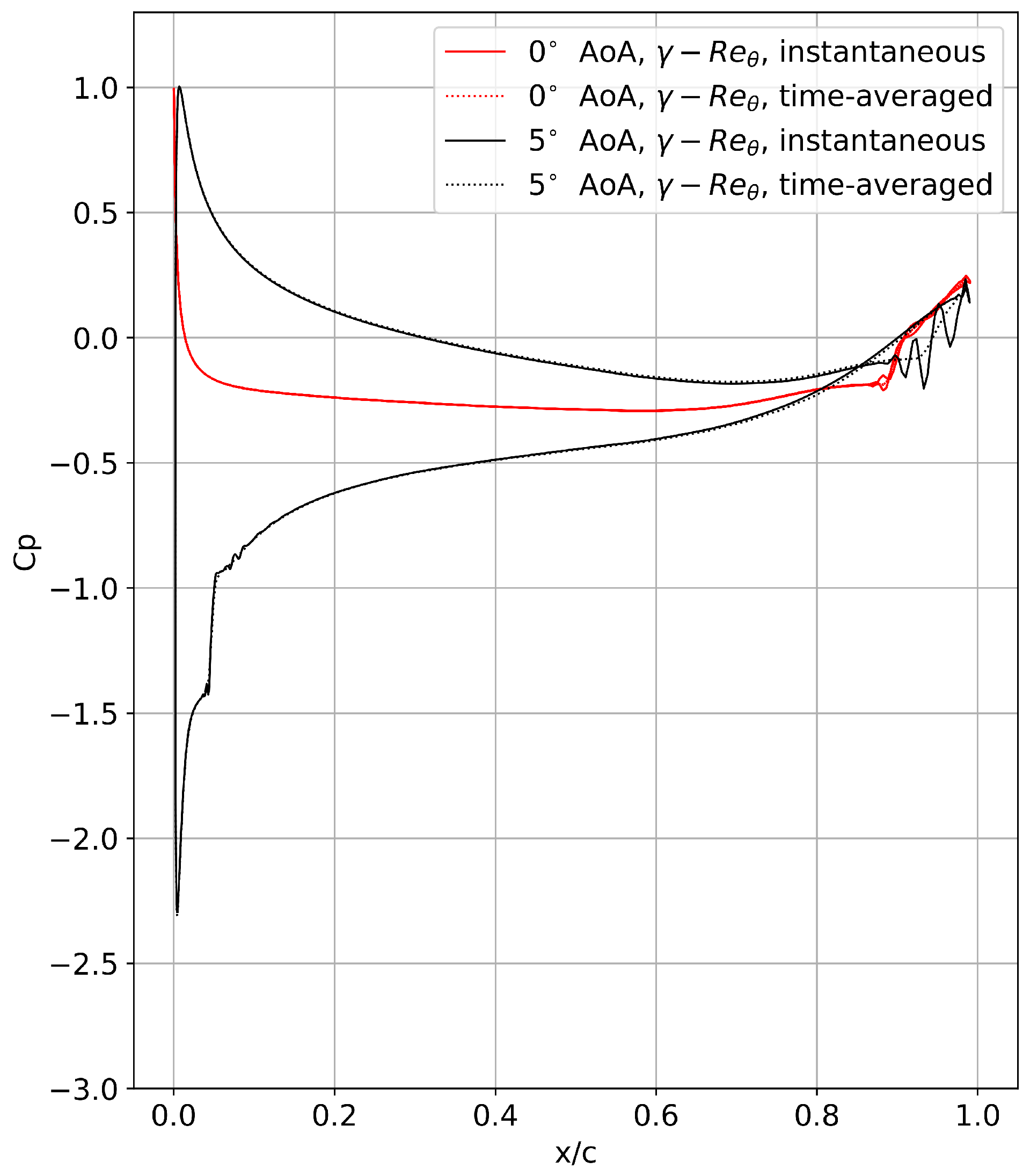
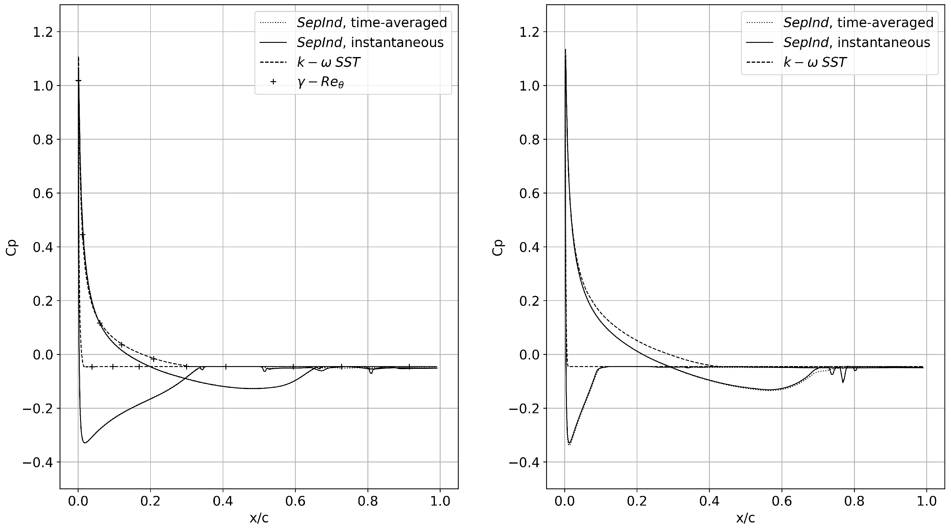
Figure 7.
Predicted pressure coefficients at AoA of and , Re = 300,000.
Figure 7.
Predicted pressure coefficients at AoA of and , Re = 300,000.
Figure 8.
Predicted pressure coefficients at AoA of and , Re = 1,000,000.
Figure 8.
Predicted pressure coefficients at AoA of and , Re = 1,000,000.
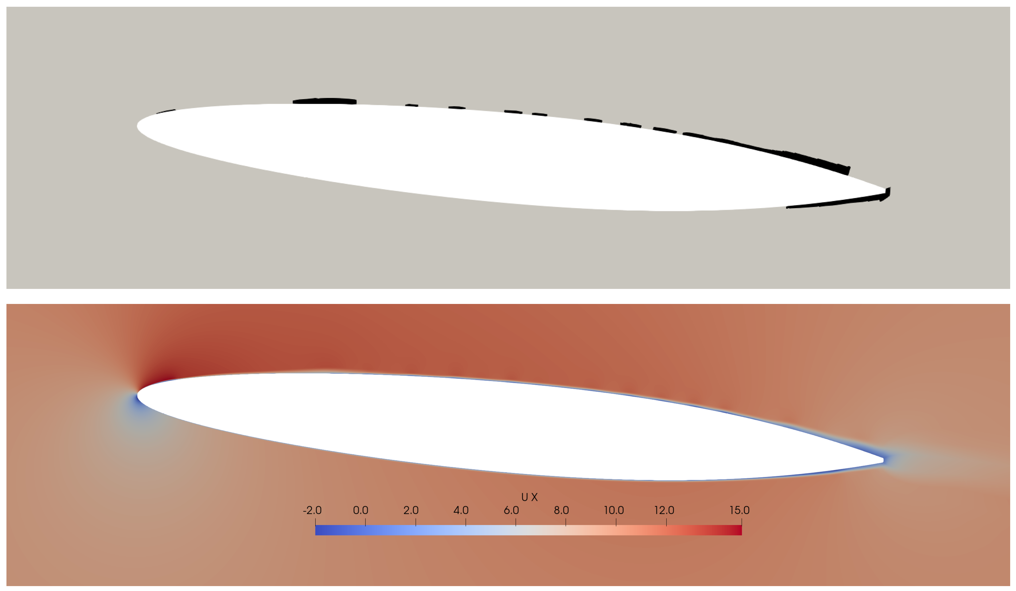
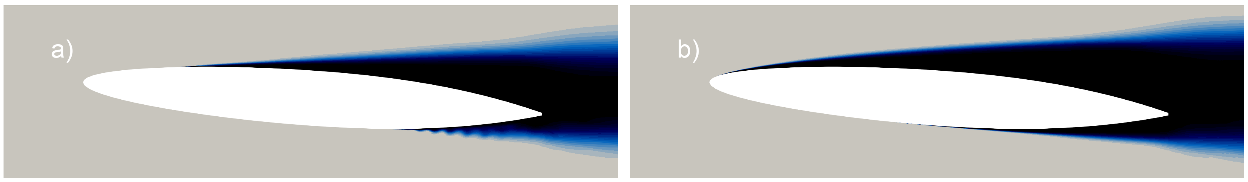
Figure 9.
Predicted non-cavitating (marked in black) and streamwise velocity at Reynolds number of 1,000,000, 2D simulation.
Figure 9.
Predicted non-cavitating (marked in black) and streamwise velocity at Reynolds number of 1,000,000, 2D simulation.
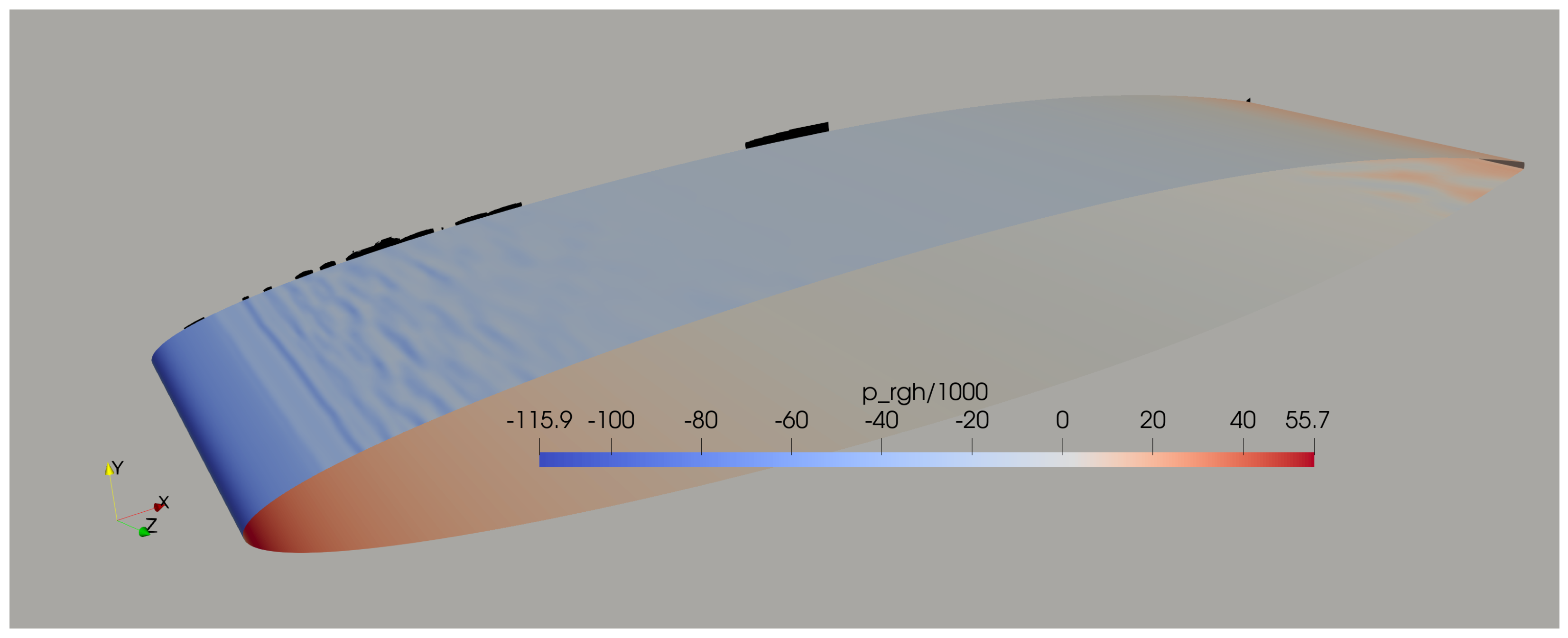
Figure 10.
Predicted non-cavitating (marked in black) and pressure on foil surface at Reynolds number of 1,000,000, 3D simulation.
Figure 10.
Predicted non-cavitating (marked in black) and pressure on foil surface at Reynolds number of 1,000,000, 3D simulation.
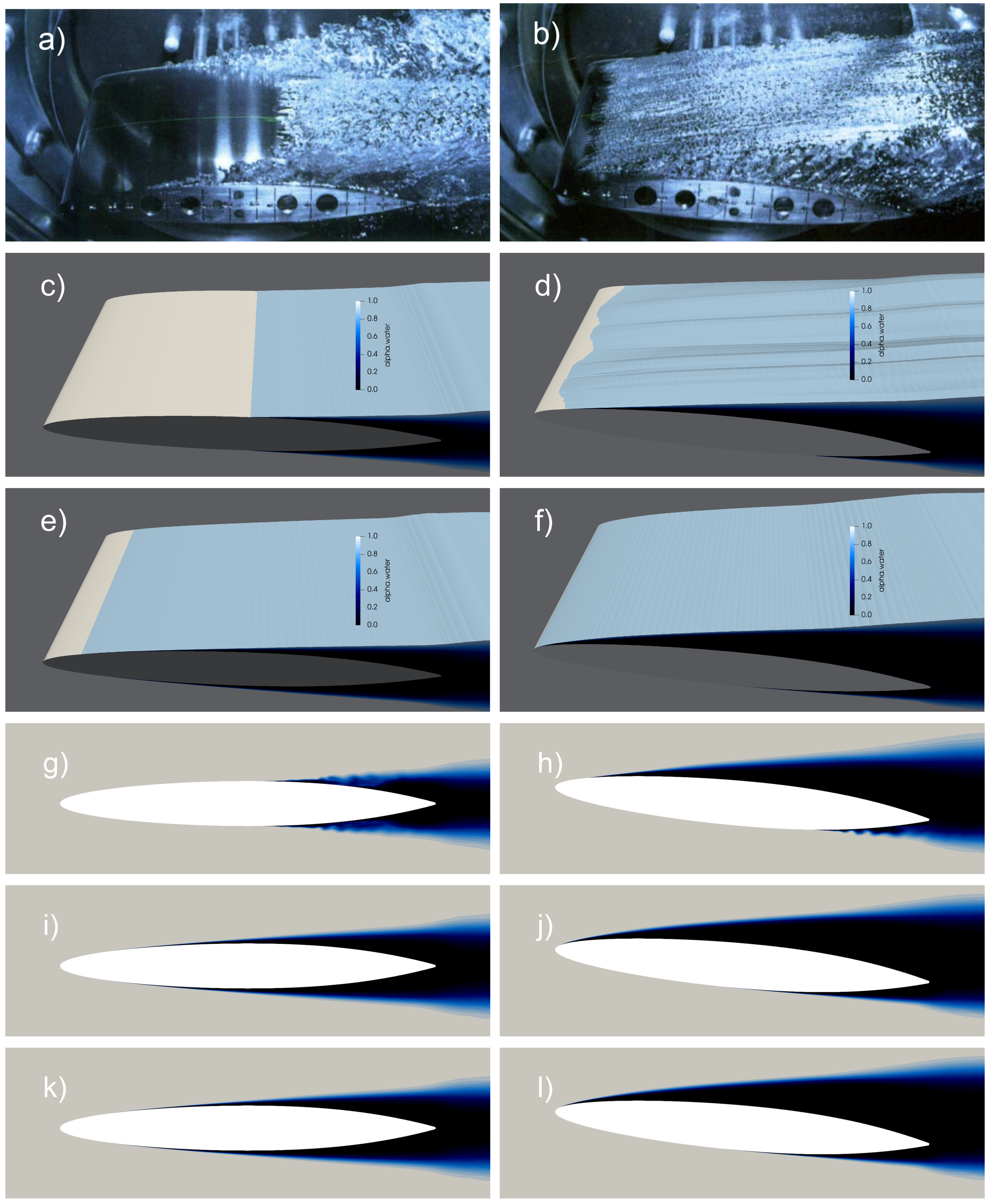
Figure 11.
Cavitation patterns on NACA 16012 at AoA of (left column) and (right column) with = 1,000,000; = 0.045. From top to bottom: (a,b) experimental photos; (c,d) bridged model, 3D; (e,f) , 3D; (g,h) bridged model, 2D; (i,j) , 2D; (k,l) , 2D.
Figure 11.
Cavitation patterns on NACA 16012 at AoA of (left column) and (right column) with = 1,000,000; = 0.045. From top to bottom: (a,b) experimental photos; (c,d) bridged model, 3D; (e,f) , 3D; (g,h) bridged model, 2D; (i,j) , 2D; (k,l) , 2D.
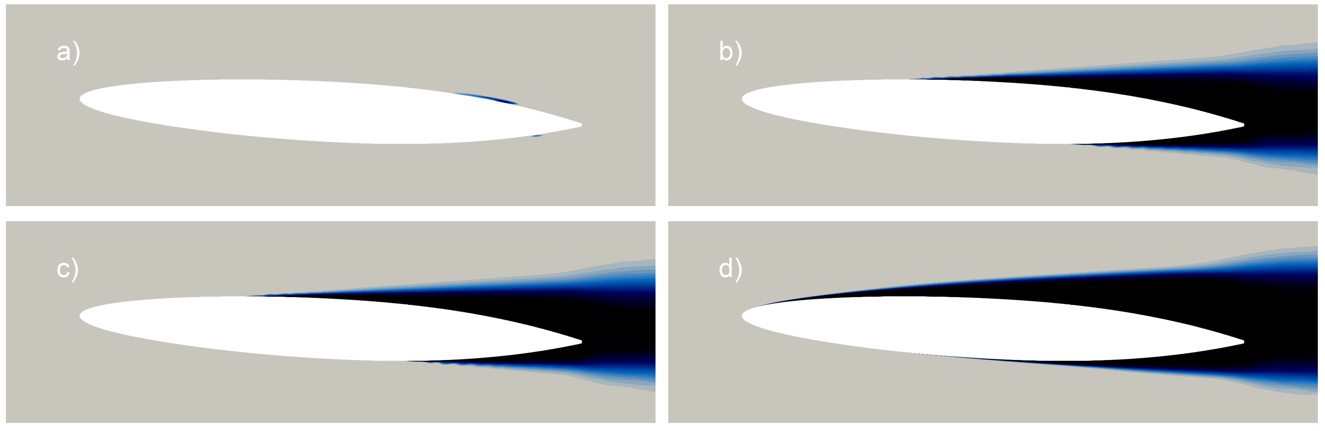
Figure 12.
Sheet cavitation development history of NACA16012, AoA = , = 1,000,000, = 0.045. (a–c) bridged model at T = 0.001 s, 0.1 s and 0.3 s. (d) unbridged at T = 0.3 s.
Figure 12.
Sheet cavitation development history of NACA16012, AoA = , = 1,000,000, = 0.045. (a–c) bridged model at T = 0.001 s, 0.1 s and 0.3 s. (d) unbridged at T = 0.3 s.
Figure 13.
Sheet cavitation prediction of NACA16012, AoA = , Re = 1,000,000, = 0.045. (a) bridged model; (b) unbridged .
Figure 13.
Sheet cavitation prediction of NACA16012, AoA = , Re = 1,000,000, = 0.045. (a) bridged model; (b) unbridged .
Figure 14.
Predicted pressure coefficients under cavitating condition for AoA = (left) and AoA = (right).
Figure 14.
Predicted pressure coefficients under cavitating condition for AoA = (left) and AoA = (right).
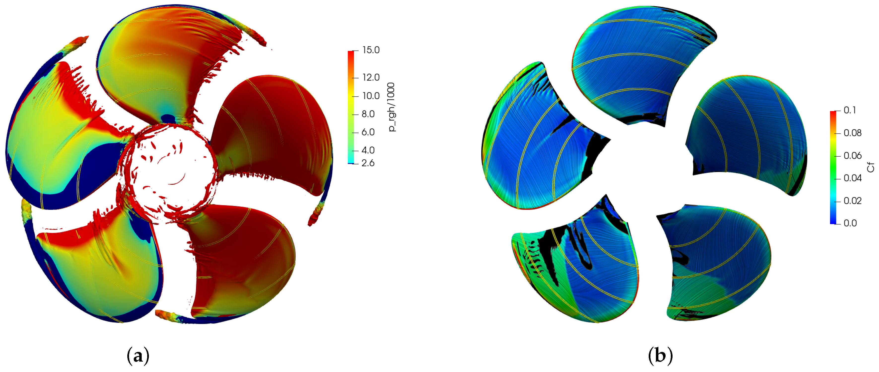
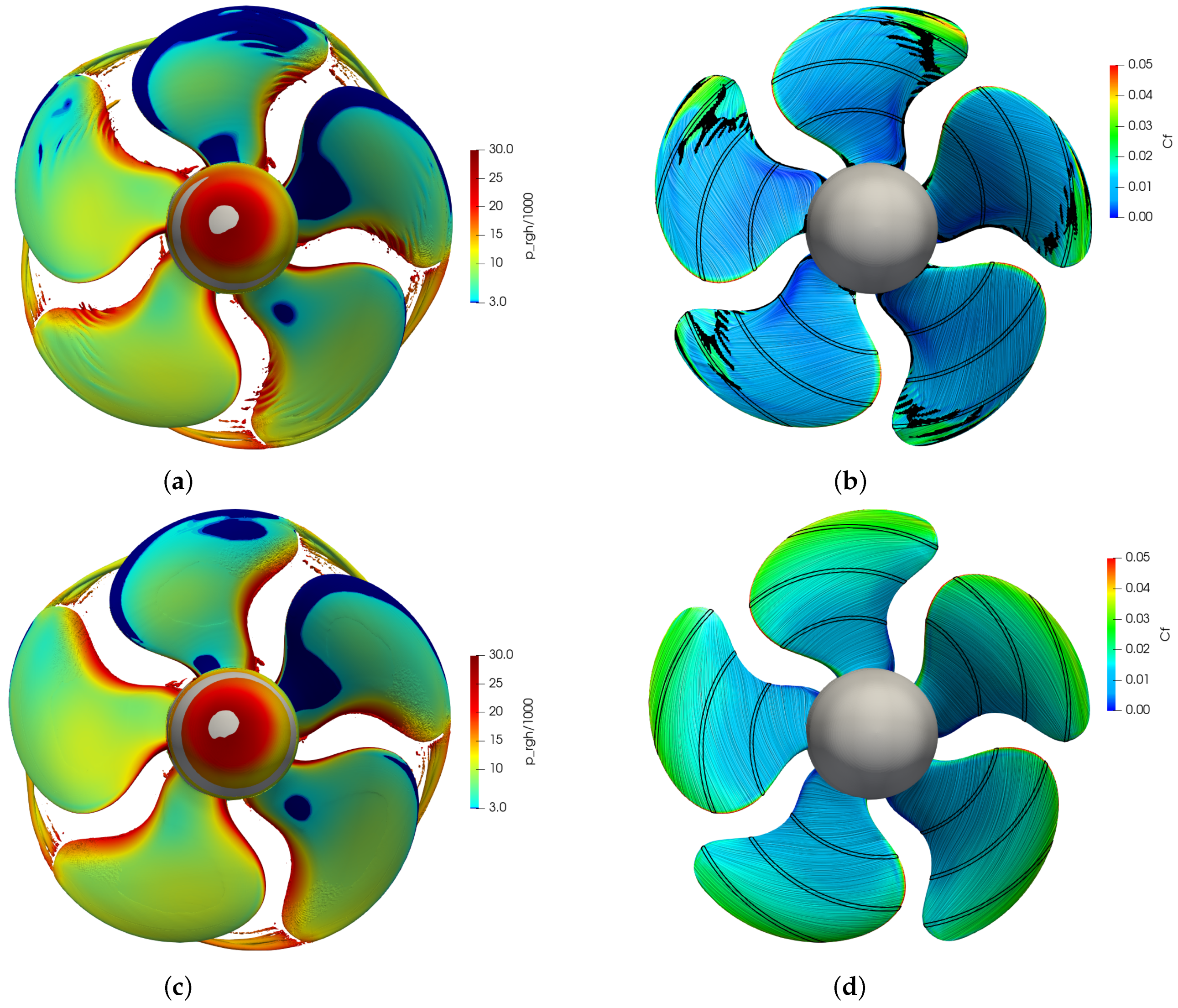
Figure 15.
PPTC VP1304 mounted on inclined shaft, J = 1.019, non-cavitating condition predictions using model with calculated . (a) Q = colored by pressure; (b) with wall limiting streamlines and contours of .
Figure 15.
PPTC VP1304 mounted on inclined shaft, J = 1.019, non-cavitating condition predictions using model with calculated . (a) Q = colored by pressure; (b) with wall limiting streamlines and contours of .
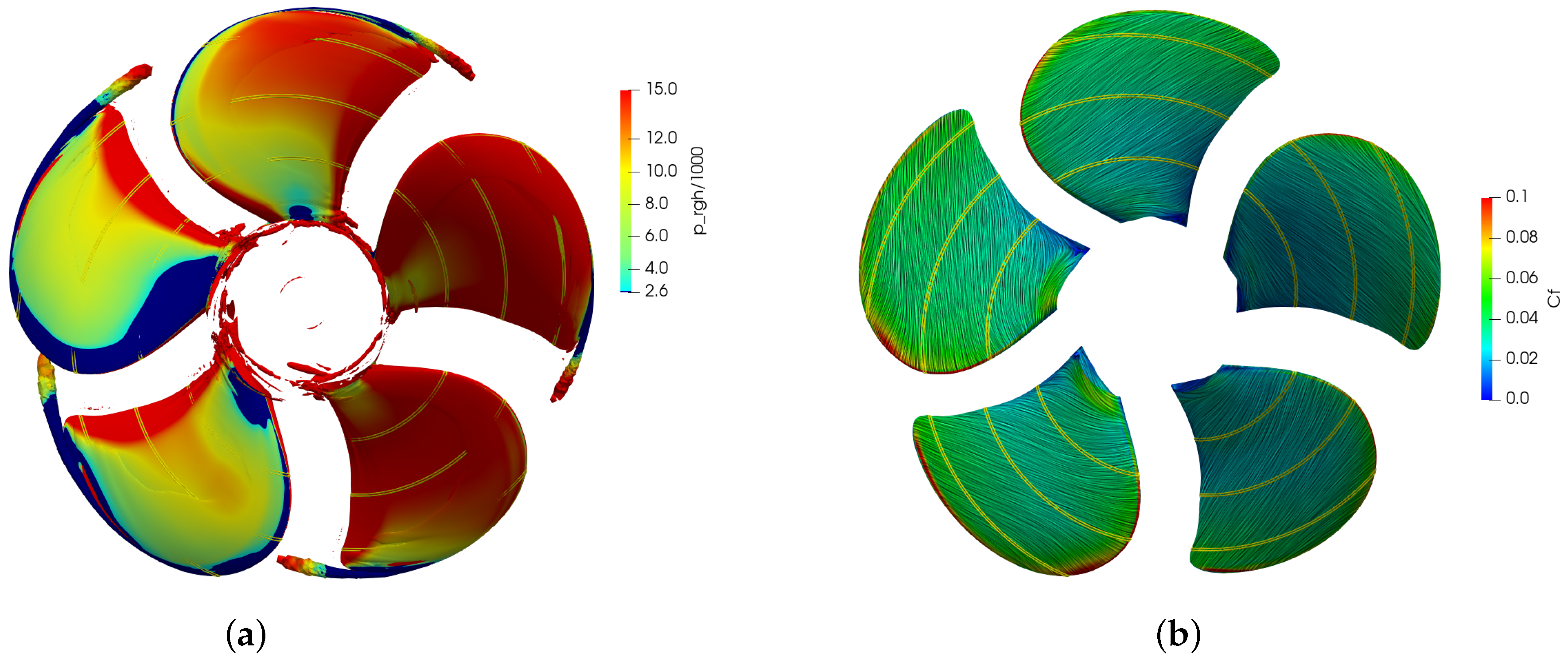
Figure 16.
PPTC VP1304 mounted on inclined shaft, J = 1.019, non-cavitating condition predictions using model. (a) Q = colored by pressure; (b) wall limiting streamlines and contours of .
Figure 16.
PPTC VP1304 mounted on inclined shaft, J = 1.019, non-cavitating condition predictions using model. (a) Q = colored by pressure; (b) wall limiting streamlines and contours of .
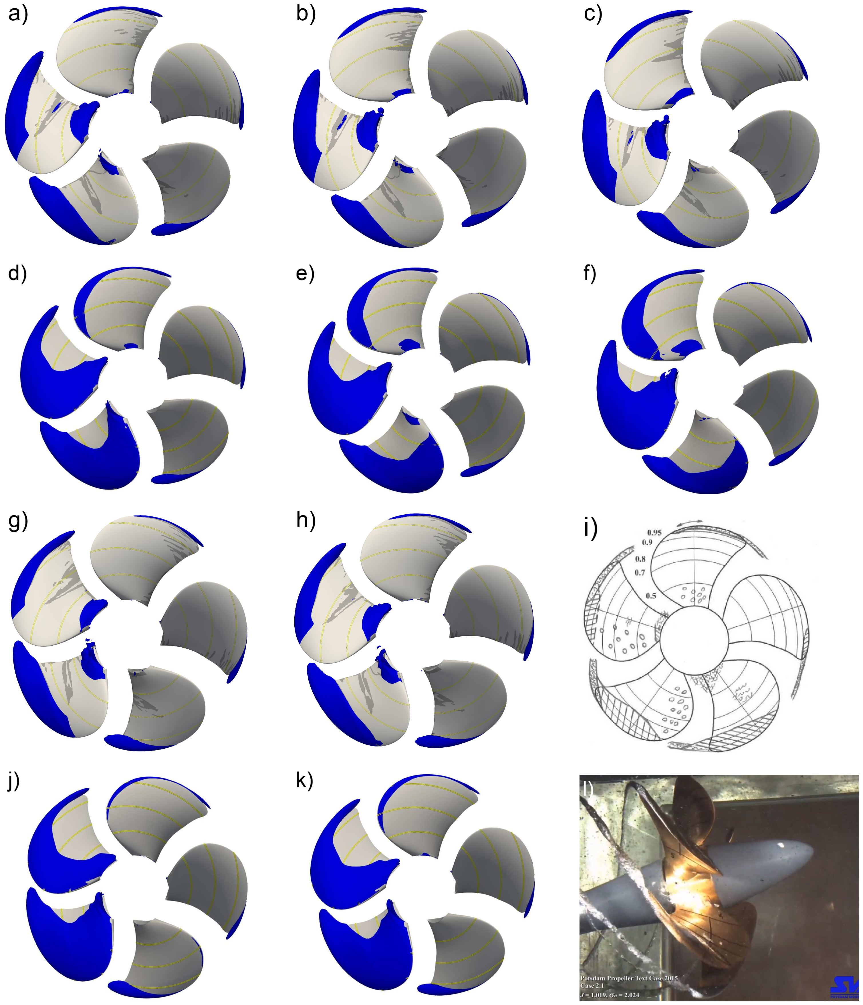
Figure 17.
Predicted cavitation pattern () using the bridged model (upper frames (a–c,g,h)) and without transition model (lower frames (d–f,j,k)) compared to the experimental sketch (i) and photo snapshot (l). (a,d) blade phase = ; (b,e): blade phase = ; (c,f) blade phase = ; (g,j) blade phase = ; (h,k) blade phase = .
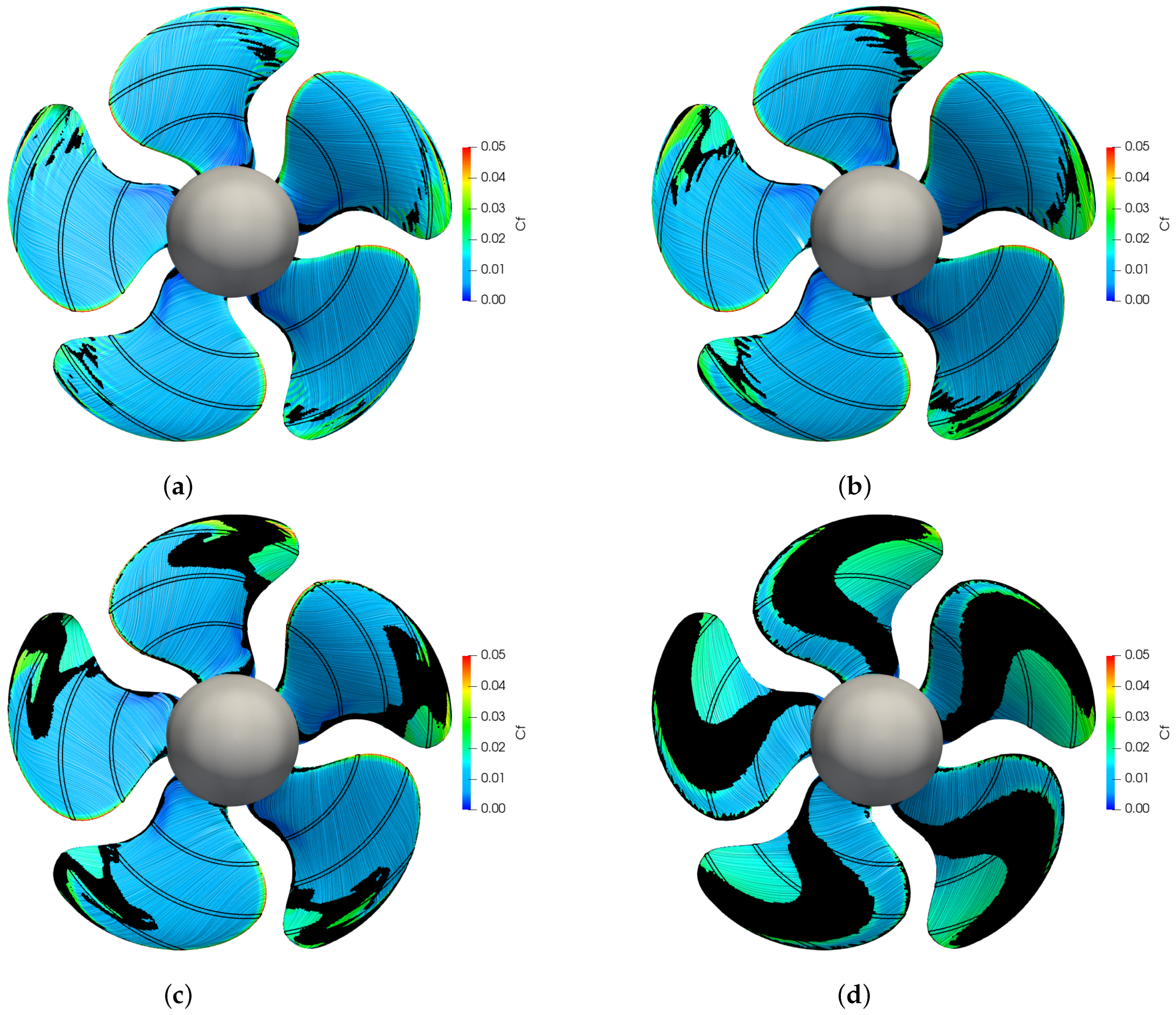
Figure 18.
Non-cavitating condition predictions. (a,c): iso-surface of Q = colored by pressure; (b,d): predicted with wall limiting streamlines colored by ; with (upper row) and (lower row) turbulence model.
Figure 18.
Non-cavitating condition predictions. (a,c): iso-surface of Q = colored by pressure; (b,d): predicted with wall limiting streamlines colored by ; with (upper row) and (lower row) turbulence model.
Figure 19.
Predicted , wall limiting streamlines and with different levels. (a) ; (b) ; (c) ; (d) .
Figure 19.
Predicted , wall limiting streamlines and with different levels. (a) ; (b) ; (c) ; (d) .
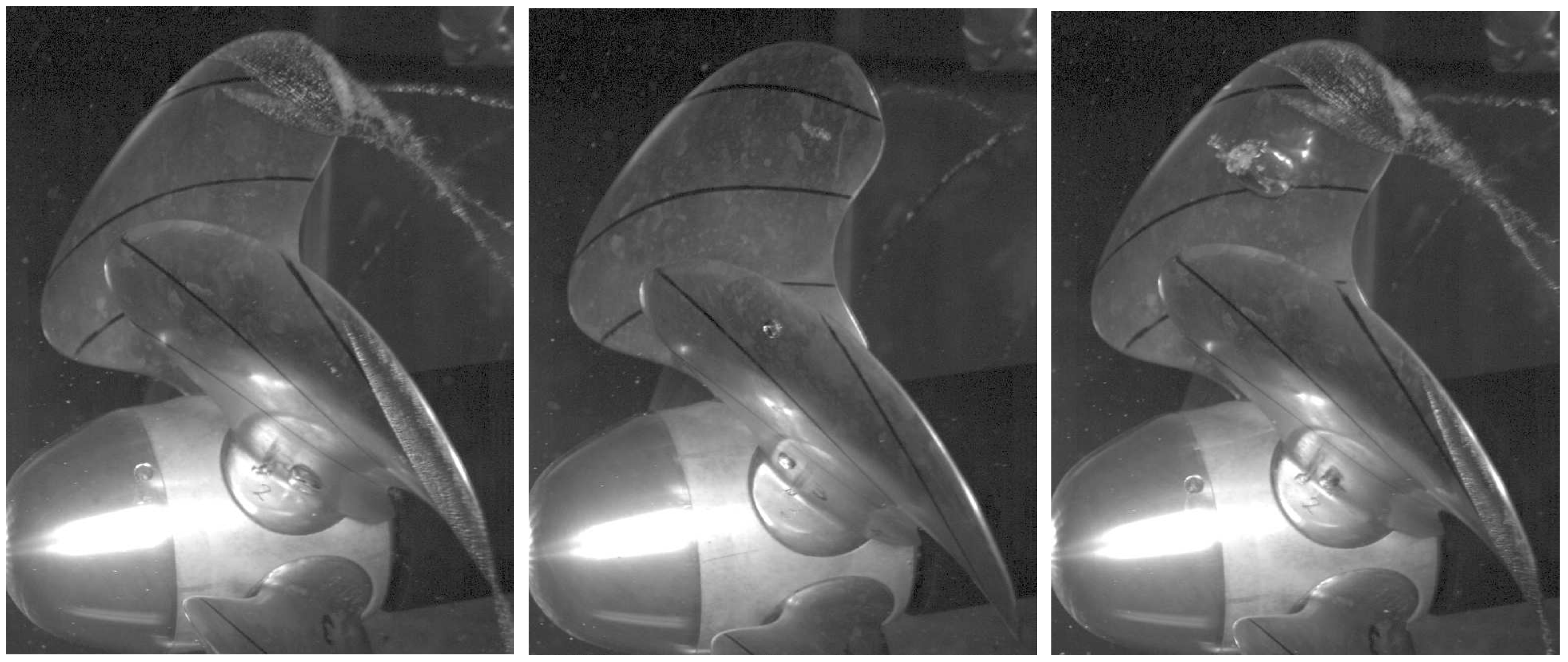
Figure 20.
Typical cavitation patterns recorded in the experiments, , . Left frame: typical cavitation pattern; middle frame: strip like cavitation on upper blade with traveling bubble on the lower blade; right frame: typical cavitation pattern with collapsing bubble.
Figure 20.
Typical cavitation patterns recorded in the experiments, , . Left frame: typical cavitation pattern; middle frame: strip like cavitation on upper blade with traveling bubble on the lower blade; right frame: typical cavitation pattern with collapsing bubble.
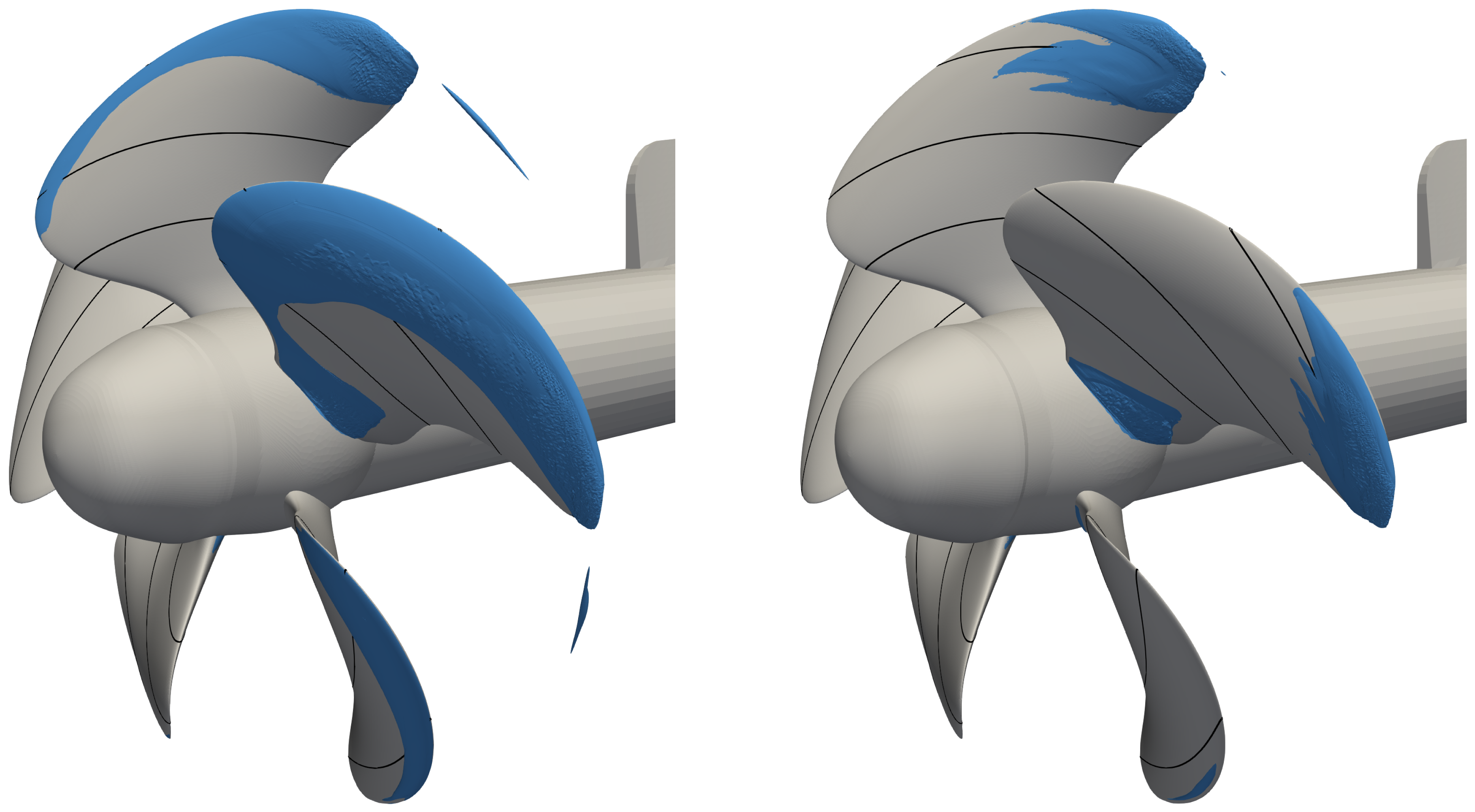
Figure 21.
Predicted cavitation patterns , , . Left frame: unbridged ; right frame: bridged model.
Figure 21.
Predicted cavitation patterns , , . Left frame: unbridged ; right frame: bridged model.
Table 1.
Studied conditions of the NACA 16012 foil.
Table 1.
Studied conditions of the NACA 16012 foil.
| Angle of Attack (AOA) | Reynolds Number | Cavitation Number | Turbulence Rate |
|---|
| 300,000 | Non-cavitating | |
| 1,000,000 | | |
| 300,000 | Non-cavitating | |
| 1,000,000 | | |
Table 2.
Inlet boundary conditions of the NACA 16012 foil.
Table 2.
Inlet boundary conditions of the NACA 16012 foil.
| Reynolds Number | U | k | | | |
|---|
| 300,000 | 3.012 | | 1.952 | | 1118 |
| 1,000,000 | 10.04 | 0.00034 | 33.885 | | 1094.8 |
Table 3.
Main characteristics of propeller VP1304.
Table 3.
Main characteristics of propeller VP1304.
| Diameter | Pitch | Chord Length (0.7 R) | Pitch Ratio (0.7 R) | Skew | No. of Blades |
|---|
| 250 mm | 408.75 mm | 104.167 mm | 1.635 | 18.8 | 5 |
Table 4.
Cell counts for case PPTC VP1304.
Table 4.
Cell counts for case PPTC VP1304.
| Region | Tets | Pyramids | Prisms | Hexes | Total |
|---|
| Inner | 11.2 Mio | 0.3 Mio | 0.06 Mio | 15.7 Mio | 27.3 Mio |
| Outer | 1.8 Mio | 0.06 Mio | 0.01 Mio | 0.5 Mio | 2.4 Mio |
| Total | 13.0 Mio | 0.36 Mio | 0.31 Mio | 16.2 Mio | 29.7 Mio |
Table 5.
Studied operating condition of VP1304.
Table 5.
Studied operating condition of VP1304.
| Advance Ratio J | Cavitation Number | Rotation Speed |
| 1.019 | 2.024 | 1200 rpm |
| Water Density | Water Kinematic Viscosity | Saturation Pressure |
| 997.78 kg/m | 9.567 × m/s | 2643 Pa |
Table 6.
Cell counts for case Kongsberg propeller A.
Table 6.
Cell counts for case Kongsberg propeller A.
| Region | Tets | Pyramids | Prisms | Hexes | Total |
|---|
| Inner | 11.7 Mio | 0.4 Mio | 0.2 Mio | 10.1 Mio | 22.4 Mio |
| Outer | 2.1 Mio | 0.1 Mio | 0.1 Mio | 1.6 Mio | 3.9 Mio |
| Total | 13.8 Mio | 0.5 Mio | 0.3 Mio | 11.7 Mio | 26.3 Mio |
Table 7.
Predicted laminar separation location and comparison to experiments, Re = 300,000.
Table 7.
Predicted laminar separation location and comparison to experiments, Re = 300,000.
| AoA | Laminar Separation Location (EXP) | Laminar Separation Location (CFD) |
|---|
| 74 ∼ 80% c | 80% c |
| 73 ∼ 77% c | 74% c |
| 40 ∼ 60% c | 67% c |
| 3 ∼ 5% c | 3 ∼ 6% c |
Table 8.
Summary of sheet cavitation inception locations.
Table 8.
Summary of sheet cavitation inception locations.
| AoA | Exp | Bridged Model | |
|---|
| 0 (2D) | 60% c | 61% c | 11% c |
| 0 (3D) | 60% c | 59% c | 11% c |
| 3 (2D) | 29–45% c | 32% c | 0.1% c |
| 4 (2D) | 13–23% c | 20.5% c | 0.1% c |
| 5 (2D) | 6–7% c | 8.7% c | 0.1% c |
| 5 (3D) | 6–7% c | 5–8% c | 0.1% c |
Table 9.
Predicted non-cavitating propulsion characteristics.
Table 9.
Predicted non-cavitating propulsion characteristics.
| Cavitation Number | | |
|---|
| EXP | non-cavitating | 0.392 | 1.010 |
| non-cavitating | 0.408 | 1.010 |
| non-cavitating | 0.393 | 0.990 |
Table 10.
Predicted cavitating propulsion characteristics.
Table 10.
Predicted cavitating propulsion characteristics.
| Cavitation Number | | | |
|---|
| EXP | 2.024 | 0.363 | 0.960 | 0.029 |
| Bridged model | 2.024 | 0.392 | 0.982 | 0.016 |
| Standard | 2.024 | 0.375 | 0.973 | 0.018 |
Table 11.
Predicted relative differences of force coefficients for propeller A, J = 0.85, non-cavitating condition.
Table 11.
Predicted relative differences of force coefficients for propeller A, J = 0.85, non-cavitating condition.
| J = 0.85 | | rdKT | rdKQ | Turbulence Model |
|---|
| | 0.1% | 2.3% | −0.29% | |
| | 0.5% | 2.5% | 0.36% | |
| | 1.0% | 2.0% | 0.39% | |
| | 3.0% | −2.3% | 0.21% | |
| | 0.5% | −2.6% | 0.24% | |


