
Scheduling of AGVs in Automated Container Terminal Based on the Deep Deterministic Policy Gradient (DDPG) Using the Convolutional Neural Network (CNN)


Abstract
:1. Introduction
2. Literature Review
3. Mathematical Model
3.1. Problem Description
3.2. Notation of the Global Parameters
3.3. AGVs Dynamic Scheduling Model
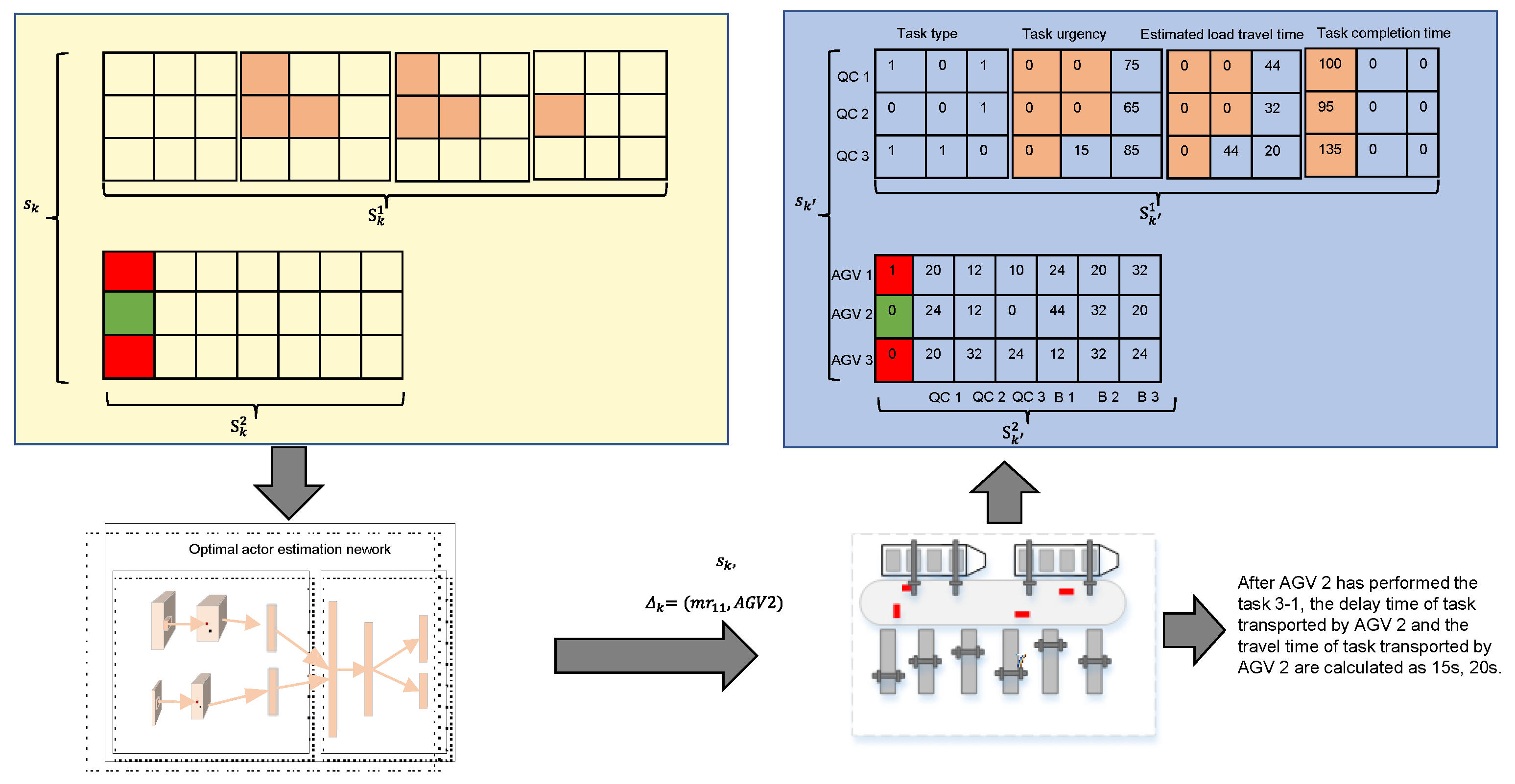
3.3.1. System State Information
- (1)
- The channel of container types is used to indicate the types of containers. In the dual-cycle mode of loading and unloading, the execution of different types of containers by the AGVs affects the synchronization of the operation of the QCs and the AGVs. For example, when the AGVs transport the importing containers, they directly travel to the QCs to pick up the container, this process only includes the empty travel time of the AGVs. When the AGVs transport and export the container, they first travel to the front of the YCs to pick up container, and then travel to the QCs to unload the container, the process includes two processing stages, so it takes longer for AGVs to reach QCs. The values 0 and 1 are used to denote the import and export boxes, respectively.
- (2)
- The channel for container urgency indicates the urgency of each container. In order to ensure the synchronization of the QCs in loading and unloading each container with the AGVs, and to reduce the delay time of containers handover, the urgency of a container can be expressed as the remaining time until the earliest possible event time. Once the container is transported, the urgency of the container is set to 0; otherwise, the urgency of the unexecuted container can be expressed as:
- (3)
- The estimated load travel time channel records the estimated load travel time for each container not transported by the AGV. The load travel time for the AGV to execute the container is estimated using an automated terminal horizontal transportation map of path network , according to the container loading and unloading location. The estimated load travel time is set to 0 if the container is assigned to the AGV for execution.
- (4)
- The completion time channel records the actual time that each container is completed, initialized to an all-0 matrix.
3.3.2. Action Space Expression
3.3.3. Reward Design and Reshaping
3.3.4. Optimal Scheduling Strategy
4. CDA Scheduling Algorithm
4.1. CDA Algorithm Network Structure
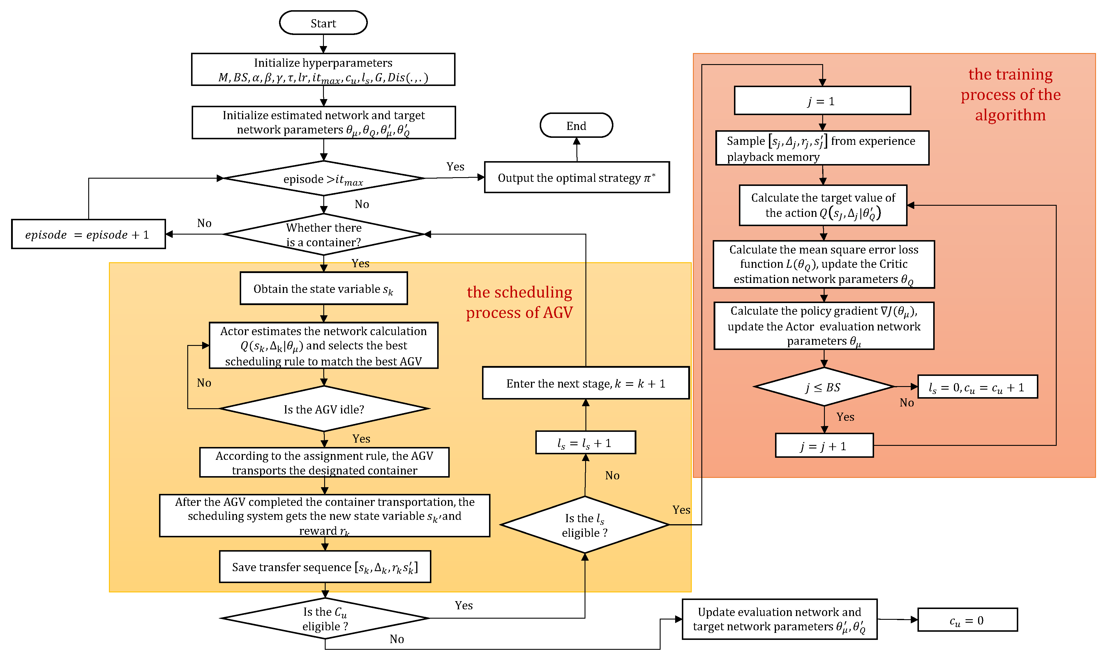
4.2. Algorithm Update Process
| Algorithm 1. Solving AGV scheduling based on CDA algorithm. |
| Input: Hyperparameters , the automated terminal horizontal transportation map of path network , transport time function Output: The optimal strategy is the optimal Actor estimation network parameter 1: Initialize estimated network and target network parameters, including 2: For episode: = 1 to 3: Scheduling system obtains state information from the AGV scheduling terminal environment 4: The Actor estimation network gives the decision action based on the state variable 5: and reward , and determines if the task is completed 6: Store the state transfer sequence into the experience replay memory 7: If meets the conditions, start training the network 8: For : = 1 to 9: Sample from the experience replay memory, and calculate the state action target value 10: Calculate the mean square error loss function and update the Critic estimation network parameters by the gradient descent algorithm 11: Use the backpropagation of the policy gradient to update the Actor target network parameters 12: End for 13: End if 14: If the condition of is met 15: Update the parameters and using the “soft” target update method 16: End if 17: End for |
4.3. Implementation of AGVs Dynamic Scheduling
5. Numerical Experiments
5.1. Experimental Parameters Setting
- (1)
- The number of container tasks considered in each episode , where 50–100 containers are considered for the small-scale problem and 100–500 containers for the large-scale problem; the number of QCs on the sea side and the number of YCs on the land side ; and the number of AGVs are considerations of this study.
- (2)
- Studying the adaptability of the scheduling algorithm in dynamic situations by introducing uncertainty in the operation time of QCs and YCs, is a consideration of this study. It is assumed that the operation time of QC, loading containers onto or unloading containers from the AGV obeys uniform distribution ; the time of the AGV loading and unloading containers at YC obeys uniform distribution .
- (3)
- This experiment takes the port operation values obtained from Xiamen Yuanhai Container Automation Terminal as a reference. The length and width of the horizontal transport area are set to 240 m and 100 m, respectively, and the speed of AGV is 5 m/s [30].
- (4)
- According to the containers and the task sequence arranged before the ship berthing, the earliest possible event time for each container task is set. The earliest possible event interval of the preceding and following tasks in the tasks sequence obeys a normal distribution , e.g., if container is the successor of container in the tasks sequence, then the earliest possible event time of container is .
5.2. Parameter Experiment
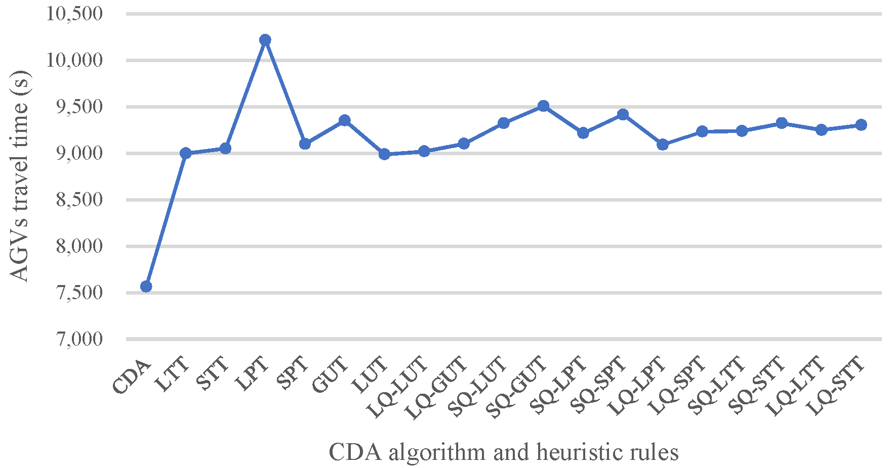
5.3. Comparison of Experimental Results
6. Conclusions and Future Research Direction
Author Contributions
Funding
Institutional Review Board Statement
Informed Consent Statement
Data Availability Statement
Conflicts of Interest
Appendix A

| Cases | Tasks Completion Time (s) | ||||||||||||||||||
|---|---|---|---|---|---|---|---|---|---|---|---|---|---|---|---|---|---|---|---|
| LTT | STT | LPT | SPT | GUT | LUT | LQ-LUT | LQ-GUT | SQ-LUT | SQ-GUT | SQ-LPT | SQ-SPT | LQ-LPT | LQ-SPT | SQ-LTT | SQ-STT | LQ-LTT | LQ-STT | CDA | |
| 1 | 933 | 917 | 985 | 912 | 956 | 904 | 945 | 958 | 983 | 963 | 937 | 1034 | 991 | 962 | 959 | 1031 | 964 | 1008 | 826 |
| 2 | 609 | 575 | 659 | 627 | 625 | 601 | 592 | 581 | 632 | 638 | 625 | 648 | 565 | 654 | 619 | 651 | 578 | 610 | 513 |
| 3 | 938 | 973 | 1020 | 959 | 933 | 912 | 939 | 907 | 1014 | 999 | 979 | 1030 | 951 | 941 | 996 | 1031 | 946 | 1004 | 760 |
| 4 | 909 | 919 | 1015 | 932 | 913 | 884 | 926 | 959 | 978 | 985 | 954 | 984 | 954 | 975 | 959 | 990 | 912 | 953 | 809 |
| 5 | 723 | 780 | 782 | 749 | 747 | 737 | 734 | 767 | 773 | 755 | 719 | 761 | 748 | 753 | 733 | 764 | 724 | 733 | 691 |
| 6 | 759 | 787 | 844 | 755 | 765 | 776 | 811 | 805 | 772 | 806 | 760 | 773 | 806 | 772 | 774 | 769 | 785 | 754 | 662 |
| 7 | 918 | 907 | 1009 | 904 | 909 | 936 | 911 | 943 | 950 | 989 | 906 | 957 | 897 | 949 | 910 | 942 | 905 | 946 | 799 |
| 8 | 928 | 993 | 1064 | 960 | 982 | 935 | 938 | 957 | 984 | 989 | 965 | 994 | 940 | 996 | 974 | 989 | 953 | 978 | 806 |
| 9 | 756 | 809 | 868 | 761 | 781 | 774 | 776 | 768 | 760 | 808 | 748 | 792 | 766 | 797 | 750 | 761 | 761 | 783 | 637 |
| 10 | 781 | 804 | 884 | 792 | 800 | 785 | 786 | 815 | 823 | 806 | 818 | 822 | 776 | 837 | 818 | 826 | 809 | 775 | 680 |
| Cases | Tasks Delay Time (s) | ||||||||||||||||||
|---|---|---|---|---|---|---|---|---|---|---|---|---|---|---|---|---|---|---|---|
| LTT | STT | LPT | SPT | GUT | LUT | LQ-LUT | LQ-GUT | SQ-LUT | SQ-GUT | SQ-LPT | SQ-SPT | LQ-LPT | LQ-SPT | SQ-LTT | SQ-STT | LQ-LTT | LQ-STT | CDA | |
| 1 | 4228 | 1924 | 4809 | 3713 | 367 | 3585 | 6239 | 1423 | 4333 | 2451 | 3417 | 3234 | 4089 | 1861 | 3175 | 3107 | 2917 | 3209 | 1328 |
| 2 | 902 | 1435 | 1472 | 188 | 355 | 1450 | 2915 | 205 | 1774 | 1526 | 1420 | 1372 | 938 | 1583 | 1109 | 1228 | 297 | 1717 | 491 |
| 3 | 3841 | 2839 | 4898 | 3890 | 384 | 4122 | 7071 | 145 | 3559 | 3664 | 3177 | 2963 | 3269 | 2768 | 2693 | 2801 | 1203 | 2506 | 1360 |
| 4 | 7760 | 5092 | 9244 | 6425 | 1002 | 9376 | 12,254 | 1669 | 7252 | 5368 | 6334 | 6270 | 7098 | 6170 | 6147 | 6145 | 5886 | 6921 | 2731 |
| 5 | 3732 | 4167 | 4623 | 4019 | 522 | 5998 | 7732 | 412 | 5222 | 2940 | 4211 | 4579 | 3821 | 4260 | 4136 | 4519 | 2391 | 4459 | 2648 |
| 6 | 4779 | 5266 | 5147 | 5954 | 725 | 5622 | 8823 | 975 | 4983 | 4413 | 4301 | 4275 | 4469 | 5124 | 4242 | 4225 | 3543 | 6313 | 1633 |
| 7 | 6269 | 6158 | 8639 | 7111 | 829 | 9513 | 12,695 | 918 | 7410 | 6083 | 6338 | 6375 | 6523 | 5643 | 5990 | 6398 | 4580 | 6739 | 3345 |
| 8 | 6447 | 6771 | 8114 | 6861 | 1017 | 10,016 | 12,952 | 2810 | 5799 | 5537 | 4891 | 4692 | 7550 | 6570 | 4693 | 4441 | 7535 | 10453 | 2746 |
| 9 | 4899 | 3627 | 6896 | 4255 | 707 | 6973 | 9717 | 337 | 4881 | 2650 | 4174 | 4279 | 5274 | 3430 | 4162 | 3972 | 4096 | 4793 | 1739 |
| 10 | 6316 | 3261 | 6989 | 5772 | 587 | 6163 | 8672 | 931 | 5640 | 3153 | 5233 | 4931 | 5546 | 3010 | 5319 | 4720 | 4930 | 5366 | 1800 |
| Cases | AGVs Travel Time (s) | ||||||||||||||||||
|---|---|---|---|---|---|---|---|---|---|---|---|---|---|---|---|---|---|---|---|
| LTT | STT | LPT | SPT | GUT | LUT | LQ-LUT | LQ-GUT | SQ-LUT | SQ-GUT | SQ-LPT | SQ-SPT | LQ-LPT | LQ-SPT | SQ-LTT | SQ-STT | LQ-LTT | LQ-STT | CDA | |
| 1 | 4530 | 4379 | 4882 | 4380 | 4595 | 4294 | 4599 | 4637 | 4734 | 4746 | 4634 | 4862 | 4724 | 4565 | 4606 | 4874 | 4602 | 4730 | 3901 |
| 2 | 4483 | 4229 | 4853 | 4460 | 4609 | 4450 | 4431 | 4331 | 4616 | 4666 | 4604 | 4752 | 4336 | 4676 | 4604 | 4752 | 4387 | 4405 | 3779 |
| 3 | 7149 | 7212 | 8030 | 7291 | 7173 | 6991 | 7125 | 7013 | 7673 | 7605 | 7493 | 7833 | 7278 | 7199 | 7445 | 7913 | 7312 | 7493 | 5937 |
| 4 | 7025 | 6994 | 7921 | 7043 | 7077 | 6811 | 7108 | 7101 | 7384 | 7362 | 7330 | 7514 | 7210 | 7381 | 7300 | 7520 | 6983 | 7274 | 6048 |
| 5 | 6919 | 7061 | 7707 | 7033 | 7095 | 6982 | 6984 | 7043 | 7193 | 7097 | 7019 | 7219 | 7091 | 7093 | 7045 | 7223 | 6833 | 7033 | 6412 |
| 6 | 7041 | 7263 | 8064 | 7264 | 7311 | 7148 | 7452 | 7545 | 7350 | 7709 | 7295 | 7358 | 7396 | 7277 | 7239 | 7352 | 7277 | 7259 | 6093 |
| 7 | 8735 | 8685 | 9682 | 8691 | 8807 | 8620 | 8641 | 8953 | 8975 | 9309 | 8929 | 9135 | 8605 | 8933 | 8835 | 9141 | 8695 | 8733 | 7569 |
| 8 | 8999 | 9053 | 10,220 | 9101 | 9353 | 8988 | 9021 | 9103 | 9325 | 9509 | 9217 | 9417 | 9093 | 9234 | 9241 | 9323 | 9251 | 9304 | 7565 |
| 9 | 8628 | 8724 | 9815 | 8677 | 8809 | 8741 | 8883 | 8722 | 8735 | 8997 | 8645 | 8927 | 8719 | 8761 | 8631 | 8825 | 8756 | 8642 | 7325 |
| 10 | 8888 | 8785 | 9941 | 8823 | 8948 | 8824 | 8811 | 8960 | 9264 | 9835 | 9304 | 9334 | 8899 | 9168 | 9350 | 9308 | 9075 | 8795 | 7482 |
| Cases | Tasks Delay Rate | ||||||||||||||||||
|---|---|---|---|---|---|---|---|---|---|---|---|---|---|---|---|---|---|---|---|
| LTT | STT | LPT | SPT | GUT | LUT | LQ-LUT | LQ-GUT | SQ-LUT | SQ-GUT | SQ-LPT | SQ-SPT | LQ-LPT | LQ-SPT | SQ-LTT | SQ-STT | LQ-LTT | LQ-STT | CDA | |
| 1 | 0.24 | 0.18 | 0.24 | 0.2 | 0.14 | 0.12 | 0.26 | 0.10 | 0.22 | 0.18 | 0.18 | 0.24 | 0.22 | 0.14 | 0.20 | 0.22 | 0.16 | 0.22 | 0.10 |
| 2 | 0.12 | 0.14 | 0.16 | 0.10 | 0.10 | 0.10 | 0.20 | 0.06 | 0.16 | 0.16 | 0.14 | 0.14 | 0.14 | 0.14 | 0.14 | 0.14 | 0.10 | 0.10 | 0.08 |
| 3 | 0.123 | 0.14 | 0.15 | 0.14 | 0.09 | 0.09 | 0.19 | 0.04 | 0.10 | 0.15 | 0.09 | 0.09 | 0.14 | 0.14 | 0.08 | 0.09 | 0.09 | 0.10 | 0.08 |
| 4 | 0.29 | 0.21 | 0.34 | 0.28 | 0.28 | 0.21 | 0.34 | 0.13 | 0.26 | 0.25 | 0.24 | 0.26 | 0.30 | 0.24 | 0.24 | 0.25 | 0.25 | 0.24 | 0.20 |
| 5 | 0.19 | 0.21 | 0.24 | 0.21 | 0.19 | 0.15 | 0.25 | 0.09 | 0.21 | 0.22 | 0.20 | 0.19 | 0.16 | 0.18 | 0.20 | 0.19 | 0.18 | 0.21 | 0.18 |
| 6 | 0.23 | 0.19 | 0.25 | 0.21 | 0.19 | 0.15 | 0.28 | 0.13 | 0.20 | 0.21 | 0.20 | 0.20 | 0.24 | 0.21 | 0.20 | 0.20 | 0.19 | 0.23 | 0.13 |
| 7 | 0.22 | 0.18 | 0.22 | 0.22 | 0.19 | 0.15 | 0.29 | 0.07 | 0.21 | 0.20 | 0.22 | 0.20 | 0.25 | 0.17 | 0.20 | 0.20 | 0.19 | 0.21 | 0.15 |
| 8 | 0.20 | 0.18 | 0.27 | 0.22 | 0.20 | 0.17 | 0.28 | 0.12 | 0.22 | 0.18 | 0.20 | 0.20 | 0.20 | 0.19 | 0.20 | 0.18 | 0.20 | 0.22 | 0.14 |
| 9 | 0.18 | 0.16 | 0.17 | 0.15 | 0.15 | 0.14 | 0.25 | 0.08 | 0.18 | 0.14 | 0.15 | 0.17 | 0.19 | 0.17 | 0.15 | 0.17 | 0.17 | 0.16 | 0.12 |
| 10 | 0.22 | 0.14 | 0.20 | 0.20 | 0.15 | 0.13 | 0.24 | 0.09 | 0.20 | 0.14 | 0.20 | 0.18 | 0.20 | 0.13 | 0.20 | 0.18 | 0.20 | 0.20 | 0.12 |


| Cases | Tasks Completion Time (s) | Tasks Delay Time (s) | AGVs Travel Time (s) | Delay Rate of Tasks | |||||||||||
|---|---|---|---|---|---|---|---|---|---|---|---|---|---|---|---|
| AGA | RHPA | CDA | AGA | RHPA | CDA | AGA | RHPA | CDA | AGA | RHPA | CDA | ||||
| 11 | 200-10-4-6 | 1591 | 1618 | 1584 | 7694 | 12,876 | 7604 | 15,871 | 15,433 | 15,513 | 0.1085 | 0.14 | 0.11 | 0.44 | 2.15 |
| 12 | 200-10-4-8 | 1618 | 1645 | 1616 | 10,282 | 12,112 | 8343 | 15,834 | 15,518 | 15,636 | 0.1072 | 0.14 | 0.12 | 0.12 | 1.79 |
| 13 | 200-12-4-6 | 1310 | 1345 | 1330 | 9288 | 11,509 | 8533 | 15,588 | 15,106 | 15,467 | 0.1186 | 0.15 | 0.12 | −1.50 | 1.13 |
| 14 | 200-12-4-8 | 1315 | 1327 | 1305 | 5952 | 12,973 | 8439 | 15,406 | 15,327 | 15,163 | 0.1117 | 0.13 | 0.12 | 0.77 | 1.69 |
| 15 | 300-12-4-8 | 1994 | 2011 | 1960 | 13,921 | 23,110 | 17,319 | 22,567 | 22,873 | 23,070 | 0.1057 | 0.12 | 0.12 | 1.73 | 2.60 |
| 16 | 300-12-6-10 | 2065 | 1991 | 2030 | 28,736 | 29,521 | 32,325 | 24,067 | 22,915 | 23,694 | 0.1886 | 0.16 | 0.18 | 1.72 | −1.92 |
| 17 | 300-12-6-10 | 2062 | 1983 | 2010 | 23,991 | 36,527 | 31,237 | 24,026 | 23,262 | 23,446 | 0.1699 | 0.18 | 0.20 | 2.59 | −1.34 |
| 18 | 300-13-6-8 | 1838 | 1821 | 1803 | 23,171 | 25,389 | 20,073 | 23,424 | 22,654 | 22,548 | 0.1557 | 0.16 | 0.14 | 1.94 | 1.00 |
| 19 | 300-13-6-10 | 1846 | 1890 | 1779 | 29,140 | 32,153 | 24,933 | 23,676 | 22,499 | 22,682 | 0.1683 | 0.19 | 0.17 | 3.77 | 6.24 |
| 20 | 300-13-8-10 | 1828 | 1829 | 1807 | 26,471 | 36,714 | 26,131 | 22,993 | 22,922 | 22,872 | 0.2014 | 0.21 | 0.21 | 1.16 | 1.22 |
| 21 | 400-13-6-8 | 2398 | 2435 | 2320 | 43,908 | 47,248 | 35,032 | 30,865 | 29,290 | 29,538 | 0.1,455 | 0.17 | 0.14 | 3.36 | 4.96 |
| 22 | 400-13-6-10 | 2471 | 2459 | 2384 | 37,124 | 52,999 | 47,076 | 30,935 | 30,198 | 31,038 | 0.1501 | 0.18 | 0.17 | 3.65 | 3.15 |
| 23 | 400-13-8-10 | 2374 | 2379 | 2337 | 55,548 | 64,424 | 57,329 | 30,011 | 30,033 | 29,902 | 0.243 | 0.24 | 0.19 | 1.58 | 1.80 |
| 24 | 400-14-6-8 | 2270 | 2224 | 2188 | 27,675 | 42,383 | 27,089 | 31,515 | 30,096 | 29,943 | 0.126 | 0.14 | 0.12 | 3.75 | 1.65 |
| 25 | 400-14-6-10 | 2282 | 2187 | 2083 | 32,490 | 43,594 | 34,507 | 30,617 | 29,822 | 29,820 | 0.1397 | 0.15 | 0.14 | 9.55 | 4.99 |
| 26 | 400-14-8-10 | 2265 | 2228 | 2175 | 58,538 | 48,992 | 44,950 | 31,033 | 30,217 | 29,870 | 0.2191 | 0.18 | 0.21 | 4.13 | 2.44 |
| 27 | 500-14-6-8 | 2817 | 2775 | 2649 | 46,780 | 75,977 | 66,679 | 37,914 | 37,388 | 38,196 | 0.1315 | 0.17 | 0.15 | 6.34 | 4.76 |
| 28 | 500-14-6-10 | 2832 | 2794 | 2708 | 55,802 | 64,888 | 41,159 | 38,436 | 38,102 | 38,247 | 0.1461 | 0.15 | 0.13 | 4.58 | 3.18 |
| 29 | 500-14-8-10 | 2764 | 2705 | 2611 | 68,922 | 94,360 | 73,322 | 37,949 | 36,953 | 37,204 | 0.1852 | 0.2 | 0.2 | 5.86 | 3.60 |
| 30 | 500-15-8-10 | 2722 | 2632 | 2558 | 73,674 | 78,205 | 76,810 | 38,937 | 38,548 | 37,876 | 0.1691 | 0.2 | 0.19 | 6.41 | 2.98 |
References
- Luo, J.; Wu, Y. Scheduling of container-handling equipment during the loading process at an automated container terminal. Comput. Ind. Eng. 2020, 149, 106848. [Google Scholar] [CrossRef]
- Saidi-Mehrabad, M.; Dehnavi-Arani, S.; Evazabadian, F.; Mahmoodian, V. An Ant Colony Algorithm (ACA) for solving the new integrated model of job shop scheduling and conflict-free routing of AGVs. Comput. Ind. Eng. 2015, 86, 2–13. [Google Scholar] [CrossRef]
- Xu, B.; Jie, D.; Li, J.; Yang, Y.; Wen, F.; Song, H. Integrated scheduling optimization of U-shaped automated container terminal under loading and unloading mode. Comput. Ind. Eng. 2021, 162, 107695. [Google Scholar] [CrossRef]
- Li, J.; Yang, J.; Xu, B.; Yang, Y.; Wen, F.; Song, H. Hybrid Scheduling for Multi-Equipment at U-Shape Trafficked Automated Terminal Based on Chaos Particle Swarm Optimization. J. Mar. Sci. Eng. 2021, 9, 1080. [Google Scholar] [CrossRef]
- Kim, K.H.; Bae, J.W. A look-ahead dispatching method for automated guided vehicles in automated port container terminals. Transp. Sci. 2004, 38, 224–234. [Google Scholar] [CrossRef]
- Iris, Ç.; Christensen, J.; Pacino, D.; Ropke, S. Flexible ship loading problem with transfer vehicle assignment and scheduling. Transp. Res. Part B Methodol. 2018, 111, 113–134. [Google Scholar] [CrossRef] [Green Version]
- Iris, Ç.; Lam, J.S.L. Recoverable robustness in weekly berth and quay crane planning. Transp. Res. Part B Methodol. 2019, 122, 365–389. [Google Scholar] [CrossRef]
- Degris, T.; White, M.; Sutton, R.S. Off-policy actor-critic. arXiv 2012, arXiv:1205.4839. [Google Scholar]
- Rashidi, H.; Tsang, E.P.K. A complete and an incomplete algorithm for automated guided vehicle scheduling in container terminals. Comput. Math. Appl. 2011, 61, 630–641. [Google Scholar] [CrossRef]
- Grunow, M.; Günther, H.O.; Lehmann, M. Strategies for dispatching AGVs at automated seaport container terminals. In Container Terminals and Cargo Systems; Springer: Berlin/Heidelberg, Germany, 2007; pp. 155–178. [Google Scholar]
- Pjevčević, D.; Vladisavljević, I.; Vukadinović, K.; Teodorović, D. Application of DEA to the analysis of AGV fleet operations in a port container terminal. Procedia-Soc. Behav. Sci. 2011, 20, 816–825. [Google Scholar] [CrossRef] [Green Version]
- Skinner, B.; Yuan, S.; Huang, S.; Liu, D.; Cai, B.; Dissanayake, G.; Pagac, D. Optimisation for job scheduling at automated container terminals using genetic algorithm. Comput. Ind. Eng. 2013, 64, 511–523. [Google Scholar] [CrossRef]
- Luo, J.; Wu, Y. Modelling of dual-cycle strategy for container storage and vehicle scheduling problems at automated container terminals. Transp. Res. Part E Logist. Transp. Rev. 2015, 79, 49–64. [Google Scholar] [CrossRef]
- Angeloudis, P.; Bell, M.G.H. An uncertainty-aware AGV assignment algorithm for automated container terminals. Transp. Res. Part E Logist. Transp. Rev. 2010, 46, 354–366. [Google Scholar] [CrossRef]
- Klerides, E.; Hadjiconstantinou, E. Modelling and solution approaches to the multi-load AGV dispatching problem in container terminals. Marit. Econ. Logist. 2011, 13, 371–386. [Google Scholar] [CrossRef]
- Cai, B.; Huang, S.; Liu, D.; Dissanayake, G. Rescheduling policies for large-scale task allocation of autonomous straddle carriers under uncertainty at automated container terminals. Robot. Auton. Syst. 2014, 62, 506–514. [Google Scholar] [CrossRef] [Green Version]
- Xin, J.; Negenborn, R.R.; Lodewijks, G. Rescheduling of interacting machines in automated container terminals. IFAC Proc. Vol. 2014, 47, 1698–1704. [Google Scholar] [CrossRef] [Green Version]
- Kim, J.; Choe, R.; Ryu, K.R. Multi-objective optimization of dispatching strategies for situation-adaptive AGV operation in an automated container terminal. In Proceedings of the 2013 Research in Adaptive and Convergent Systems, Montreal, QC, Canada, 1–4 October 2013; pp. 1–6. [Google Scholar] [CrossRef]
- Han, B.A.; Yang, J.J. Research on adaptive job shop scheduling problems based on dueling double DQN. IEEE Access 2020, 8, 186474–186495. [Google Scholar] [CrossRef]
- Briskorn, D.; Drexl, A.; Hartmann, S. Inventory-based dispatching of automated guided vehicles on container terminals. In Container Terminals and Cargo Systems; Springer: Berlin/Heidelberg, Germany, 2007; pp. 195–214. [Google Scholar]
- Choe, R.; Kim, J.; Ryu, K.R. Online preference learning for adaptive dispatching of AGVs in an automated container terminal. Appl. Soft Comput. 2016, 38, 647–660. [Google Scholar] [CrossRef]
- Fotuhi, F.; Huynh, N.; Vidal, J.M.; Xie, Y. Modeling yard crane operators as reinforcement learning agents. Res. Transp. Econ. 2013, 42, 3–12. [Google Scholar] [CrossRef]
- Hu, H.; Jia, X.; He, Q.; Fu, S.; Liu, K. Deep reinforcement learning based AGVs real-time scheduling with mixed rule for flexible shop floor in industry 4.0. Comput. Ind. Eng. 2020, 149, 106749. [Google Scholar] [CrossRef]
- Tang, X.; Qin, Z.; Zhang, F.; Wang, Z.; Xu, Z.; Ma, Y.; Ye, J. A deep value-network based approach for multi-driver order dispatching. In Proceedings of the 25th ACM SIGKDD International Conference on Knowledge Discovery & Data Mining, Anchorage, AK, USA, 4–8 August 2019; pp. 1780–1790. [Google Scholar] [CrossRef]
- Yao, Z.; Wang, Y.; Meng, L.; Qiu, X.; Yu, P. DDPG-Based Energy-Efficient Flow Scheduling Algorithm in Software-Defined Data Centers. Wirel. Commun. Mob. Comput. 2021, 2021, 6629852. [Google Scholar] [CrossRef]
- Luo, S.; Lin, X.; Zheng, Z. A novel CNN-DDPG based AI-trader: Performance and roles in business operations. Transp. Res. Part E Logist. Transp. Rev. 2019, 131, 68–79. [Google Scholar] [CrossRef]
- Ying, C.; Chow, A.H.F.; Chin, K.S. An actor-critic deep reinforcement learning approach for metro train scheduling with rolling stock circulation under stochastic demand. Transp. Res. Part B Methodol. 2020, 140, 210–235. [Google Scholar] [CrossRef]
- Yang, Y.; Zhong, M.; Dessouky, Y.; Postolache, O. An integrated scheduling method for AGV routing in automated container terminals. Comput. Ind. Eng. 2018, 126, 482–493. [Google Scholar] [CrossRef]
- Iqbal, S.; Sha, F. Actor-attention-critic for multi-agent reinforcement learning. International Conference on Machine Learning. arXiv 2019, arXiv:1810.02912. [Google Scholar]
- Zhong, M.; Yang, Y.; Dessouky, Y.; Postolache, O. Multi-AGV scheduling for conflict-free path planning in automated container terminals. Comput. Ind. Eng. 2020, 142, 106371. [Google Scholar] [CrossRef]
- Liu, D.; Wang, W.; Wang, L.; Jia, H.; Shi, M. Dynamic Pricing Strategy of Electric Vehicle Aggregators Based on DDPG Reinforcement Learning Algorithm. IEEE Access 2021, 9, 21556–21566. [Google Scholar] [CrossRef]
- Díaz-Madroñero, M.; Mula, J.; Jiménez, M.; Peidro, D. A rolling horizon approach for material requirement planning under fuzzy lead times. Int. J. Prod. Res. 2017, 55, 2197–2211. [Google Scholar] [CrossRef]
- Sun, Z.W. The world’s First! Zhenhua Heavy Industry Releases New Technology for Container Terminal Loading and Unloading, China Water Transport Network 2019. Available online: http://app.zgsyb.com/news.html?aid=530549 (accessed on 25 November 2021).


| Parameters | Notations |
|---|---|
| Set of AGVs, indexed by . | |
| Set of QCs, indexed by . | |
| Set of YCs, indexed by . | |
| Set of containers for QC , indexed by . | |
| Set of all containers, . | |
| The earliest possible event time container . | |
| Automated terminal horizontal transportation map of path network. | |
| The function of time for each container transported by AGV. | |
| Service time of QC loading or unloading container . | |
| Service time of YC loading or unloading container . | |
| Time interval is the final completion time of the task. | |
| Set of heuristic container allocation rule, . | |
| Action space. | |
| State space. | |
| Representation of the dimensions of the matrix. | |
| Learning rate of Actor network and Critic network. | |
| Capacity of experience replay memory. | |
| Batch size. | |
| Maximum number of episodes. | |
| Target network parameter update frequency. | |
| Algorithm training time step. | |
| Target network parameter soft update coefficient. | |
| The discount coefficient of accumulate reward. | |
| The scaling factor in the reward function. |
| Variables | Notations |
|---|---|
| . | |
| . | |
| The component of the state variable represents the information of containers. | |
| The component of the state variable represents the AGV information. | |
| . | |
| . | |
| . | |
| . | |
| The state variable of next decision stage. | |
| , which is also the completion time of the individual container task. | |
| . | |
| . | |
| . | |
| . | |
| The optimal strategy. | |
| Average delay time of all containers. | |
| Average travel time per container for AGVs transportation. | |
| Number of containers delayed. |
| Symbols | Rules | Description |
|---|---|---|
| LTT | The container with the longest transport time from origin to destination is assigned to an AGV. | |
| STT | The container with the shortest transport time from origin to destination is assigned to an AGV. | |
| GUT | The container with the greatest urgency is assigned to an AGV. | |
| LUT | The container with the least urgency is assigned to an AGV. | |
| LPT | The container with the longest processing time is assigned to an AGV; the processing time includes the time for loading and unloading the container at QCS and YCS, as well as the transportation time from the origin to the destination of the container. | |
| SPT | The container with the shortest processing time is assigned to an AGV. | |
| LQ-LTT | with the most remaining containers, from which the container with the longest transport time is selected. | |
| LQ-STT | with the most remaining containers, from which the container with the shortest transport time is selected. | |
| SQ-LTT | with the fewest remaining containers, from which the container with the longest transport time is selected. | |
| SQ-STT | with the fewest remaining containers, from which the container with the shortest transport time is selected. | |
| LQ-GUT | with the most remaining containers, from which the container with the greatest urgency is assigned to an AGV. | |
| LQ-LUT | with the most remaining containers, from which the container with the least urgency is assigned to an AGV. | |
| SQ-GUT | with the fewest remaining containers, from which the container with the greatest urgency is assigned to an AGV. | |
| SQ-LUT | with the fewest remaining containers, from which the container with the least urgency is assigned to an AGV. | |
| LQ-LPT | with the most remaining containers, from which the container with the longest processing time is assigned to the an AGV. | |
| LQ-SPT | with the most remaining containers, from which the container with the shortest processing time is assigned to an AGV. | |
| SQ-LPT | with the fewest remaining containers, from which the container with the longest processing time is assigned to an AGV. | |
| SQ-SPT | with the fewest remaining containers, from which the container with the shortest processing time is assigned to an AGV. |
| Layers | Number of Neurons | Activation Functions | Descriptions |
|---|---|---|---|
| Input layer 1 | None | . | |
| Input layer 2 | None | . | |
| Convolution layer 1 | 32 | Swish | information. |
| Pooling layer 1 | None | None | information. |
| Convolution layer 2 | 64 | Swish | information. |
| Pooling layer 2 | None | None | information. |
| Flatten layer 1 | None | None | . |
| Convolution layer 3 | 64 | Swish | information. |
| Pooling layer 3 | None | None | information. |
| Flatten layer 2 | None | None | . |
| Concatenation layer | None | None | . |
| Fully connected layer | 100 | Relu | None |
| Output layer 1 | Softmax | Output AGV information. | |
| Output layer 2 | Softmax | Output assignment rule information. | |
| Gumbel-softmax layer | 1 | None | Matching of AGV with container. |
| Layers | Number of Neurons | Activation Functions | Descriptions |
|---|---|---|---|
| Input layer 1 | None | Input of state component . | |
| Input layer 2 | None | Input of state component . | |
| Input layer 2 | 2 | None | Actor network output of action . |
| Convolution layer 1 | 32 | Swish | Extracting information. |
| Pooling layer 1 | None | None | Extracting information. |
| Convolution layer 2 | 64 | Swish | Further extraction of information. |
| Pooling layer 2 | None | None | Further extraction of information. |
| Flatten layer 1 | None | None | One-dimensionalization of . |
| Convolution layer 3 | 64 | Swish | Extracting information. |
| Pooling layer 3 | None | None | Extracting information. |
| Flatten layer 2 | None | None | One-dimensionalization of . |
| Concatenation layer 1 | None | None | Concatenation of and . |
| Concatenation layer 2 | None | None | Concatenation of and . |
| Fully connected layer 1 | 100 | Relu | None |
| Fully connected layer 2 | Relu | None | |
| Output layer | Relu | corresponding to states and actions. |
| QC ID | Task ID | Type | From Location | To Location | Earliest Event Time | Estimated Load Travel Time | Whether to Be Executed | Task Competition Time |
|---|---|---|---|---|---|---|---|---|
| QC 1 | 1-1 | 1 | B 2 | QC 1 | 70 | 32 | Y | |
| 1-2 | 0 | QC 1 | B 1 | 130 | 20 | N | ||
| 1-3 | 1 | B 3 | QC 1 | 210 | 44 | N | ||
| QC 2 | 2-1 | 0 | QC 2 | B 3 | 60 | 32 | Y | 95 |
| 2-2 | 0 | QC 2 | B 2 | 140 | 20 | Y | ||
| 2-3 | 1 | B 1 | QC 2 | 200 | 32 | N | ||
| QC 3 | 3-1 | 1 | B 2 | QC 3 | 80 | 32 | N | |
| 3-2 | 0 | QC 3 | B 1 | 150 | 44 | N | ||
| 3-3 | 1 | B 3 | QC 3 | 220 | 20 | N |
| Parameters | Parameter Values | Description of Parameters |
|---|---|---|
| 0.001 | Learning rate of Actor network and Critic network. | |
| 10,000 | Experience replay memory capacity. | |
| 32 | Batch size. | |
| 1500 | Maximum number of episodes. | |
| 100 | Target network parameter update frequency. | |
| 80 | Algorithm training time step. | |
| 0.01 | Target network parameter soft update coefficient. | |
| 0.9 | The discount coefficient of accumulative reward. |
| Reward | Delay Time of Tasks (s) | Total Travel Time of the AGV (s) | |
|---|---|---|---|
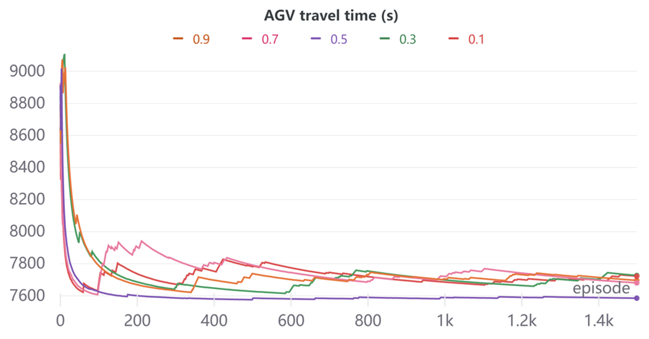
| 0.1 | 135.57 | 3194 | 7722 |
| 0.3 | 135.37 | 3264 | 7727 |
| 0.5 | 136.83 | 2848 | 7585 |
| 0.7 | 135.91 | 3103 | 7680 |
| 0.9 | 135.80 | 3133 | 7696 |
| Tasks Completion Time (s) | Tasks Delay Time (s) | AGVs Travel Time (s) | |||||||
|---|---|---|---|---|---|---|---|---|---|
| CDA | RHPA | AGA | CDA | RHPA | AGA | CDA | RHPA | AGA | |
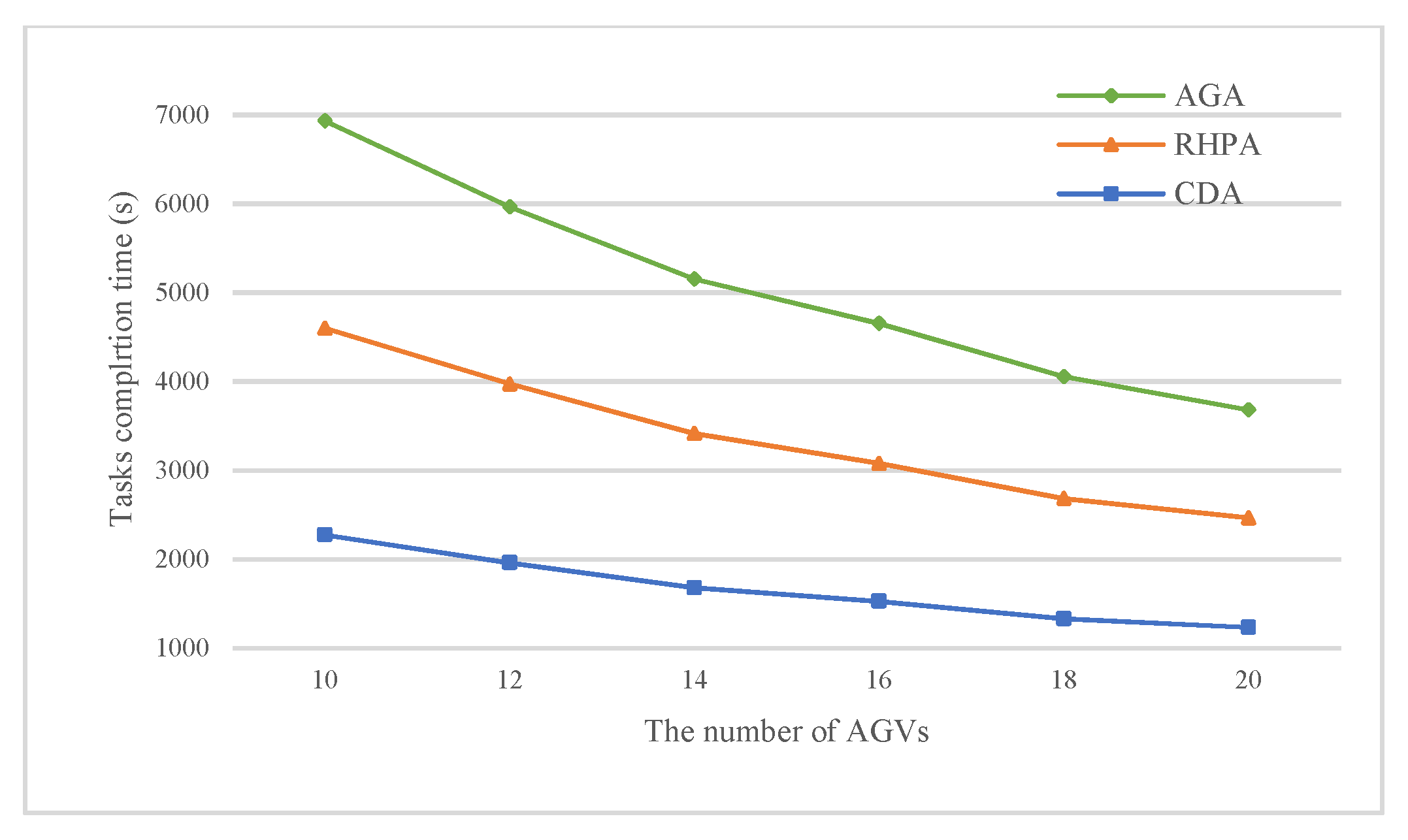
| 300-10-4-8 | 2273 | 2325 | 2332 | 23,134 | 36,705 | 23,505 | 23,357 | 23,492 | 23,016 |
| 300-12-4-8 | 1960 | 2011 | 1994 | 17,319 | 23,110 | 13,921 | 23,070 | 23,873 | 23,567 |
| 300-14-4-8 | 1679 | 1735 | 1739 | 10,731 | 19,670 | 12,810 | 23,635 | 23,902 | 23,492 |
| 300-16-4-8 | 1527 | 1552 | 1574 | 4620 | 75,215 | 7691 | 23,534 | 23,606 | 23,353 |
| 300-18-4-8 | 1331 | 1352 | 1371 | 4946 | 9494 | 6631 | 22,792 | 22,752 | 23,684 |
| 300-20-4-8 | 1234 | 1232 | 1214 | 5755 | 7466 | 6652 | 22,701 | 22,949 | 23,475 |
Publisher’s Note: MDPI stays neutral with regard to jurisdictional claims in published maps and institutional affiliations. |
© 2021 by the authors. Licensee MDPI, Basel, Switzerland. This article is an open access article distributed under the terms and conditions of the Creative Commons Attribution (CC BY) license (https://creativecommons.org/licenses/by/4.0/).
Share and Cite
Chen, C.; Hu, Z.-H.; Wang, L. Scheduling of AGVs in Automated Container Terminal Based on the Deep Deterministic Policy Gradient (DDPG) Using the Convolutional Neural Network (CNN). J. Mar. Sci. Eng. 2021, 9, 1439. https://0-doi-org.brum.beds.ac.uk/10.3390/jmse9121439
Chen C, Hu Z-H, Wang L. Scheduling of AGVs in Automated Container Terminal Based on the Deep Deterministic Policy Gradient (DDPG) Using the Convolutional Neural Network (CNN). Journal of Marine Science and Engineering. 2021; 9(12):1439. https://0-doi-org.brum.beds.ac.uk/10.3390/jmse9121439
Chicago/Turabian StyleChen, Chun, Zhi-Hua Hu, and Lei Wang. 2021. "Scheduling of AGVs in Automated Container Terminal Based on the Deep Deterministic Policy Gradient (DDPG) Using the Convolutional Neural Network (CNN)" Journal of Marine Science and Engineering 9, no. 12: 1439. https://0-doi-org.brum.beds.ac.uk/10.3390/jmse9121439