
Extreme Waves in the Agulhas Current Region Inferred from SAR Wave Spectra and the SWAN Model


Centre for Marine Technology and Ocean Engineering (CENTEC), Instituto Superior Técnico, Universidade de Lisboa, 1049-004 Lisboa, Portugal
*
Author to whom correspondence should be addressed.
J. Mar. Sci. Eng. 2021, 9(2), 153; https://0-doi-org.brum.beds.ac.uk/10.3390/jmse9020153
Submission received: 13 January 2021
/
Revised: 27 January 2021
/
Accepted: 28 January 2021
/
Published: 2 February 2021
(This article belongs to the Special Issue Extreme Waves)
Abstract
:The influence of the Agulhas Current on the wave field is investigated. The study is conducted by performing high resolution spectral wave model simulations with and without ocean currents. The validation of the numerical simulations is performed for the Significant Wave Height (Hs) using all possible satellite altimetry data available in the study region for a winter period of 2018. Wave spectra and extreme waves parameters are examined in places where waves and current are aligned in the Agulhas Current. Sentinel-1 (S1) wave mode Synthetic Aperture Radar (SAR) spectra are used to estimate the composites of the Hs and BFI (Benjamin–Feir Index). SAR computed BFI and Hs were compared with the respective composites obtained from the Simulating Waves Nearshore (SWAN) model. From the Hs composites using SAR data and modeled data, it can be concluded that the Hs maxima values are distributed in the Agulhas Current Retroflection (ACR) and also in the southern limit of the domain that is affected by the strong circumpolar winds around Antarctic. In addition, the BFI composites exhibit the highest values in the ACR and some few values are observed in the southern border as occurred with the Hs. The results of this study indicate that there is direct correlation between the Agulhas Current strength, the Hs and the BFI. It was found that the modeled directional wave spectra are broadened when the ocean current is considered in the simulation. The analysis of the modeled wave spectra is performed over eddies, rings and meanders in the Agulhas Current region. The transformation of the wave spectra due to current refraction is discussed based on the numerical simulations. The effect of the Agulhas Current on the spectral shape is explored. The spectral wave energy grows when the wave and the current are aligned, resulting in peaked, elongated and widened spectra. A decrease of the peak period was observed before the occurrence of maximum values of BFI, which characterize abnormal sea states.
1. Introduction
Bad weather is not the main cause of ship losses and it may represent a relatively small percentage of the direct causes of ship losses, as described in [1]. However, ship losses by other causes, such as fire or grounding can have bad weather as a causal factor or even as a direct cause. This has been explored by [2] who have analyzed a sample of accident records of Lloyds from 1978 to 1999 in a total of 547 reports and in these reference was made to bad weather in about 53% of the cases, which makes bad weather appear as an important effect in ship losses. Further analysis of the location of the accidents and the prevailing weather conditions showed that there was a high correlation of the accidents with the occurrence of sea states with high mean steepness.
Severe sea states have caused the loss of many ships and to improve safety in maritime operations, decision making about ship routing [3] must rely upon wave forecast that require the best available knowledge of hazardous wave environments. Improving the understanding of extreme and abnormal waves [4,5,6,7] is also very important to assess the safety of marine operations to avoid ship casualties [8,9,10,11,12,13].
In the Agulhas Current (AC), Mallory [14] examined weather circumstances under which huge waves developed and their effects on vessels. Using satellite altimetry [15] has shown that up to 17% of the investigated wave profiles showed amplification of more than 40% in the Agulhas Current.
The AC is composed of two main parts: the Northern, which is stable with velocities ranging from 1.4 to 1.6 m/s, and the Southern AC with large meanders and mesoscale eddies [16] with velocities that range from 1.5 to 2 m/s [17,18]. The Agulhas Current meanders contribute in the intensification of the thermocline on the Agulhas Bank through the intrusion of warmer water [19,20].
Having passed the Agulhas Bank, the AC overshoots the African continent prograde into the South Atlantic Ocean where it experiences a strong change in direction [21], retroflecting back into the South Indian Ocean as the Agulhas Return Current [22]. The current turns back on itself in a tight loop known as Agulhas Current Retroflection [17].
Moreover, the AC plays a key role in the inter-ocean exchange and in the global interchange of water masses [23]. In addition, one of the global oceanic circulation processes that has received attention, has been the concept of a global oceanic conveyor belt [24] in which the AC plays an important role [17]. Satellite altimetry data and SAR allowed us to investigate different aspects, behavior and features of the AC [15,19,25]. The AC region is one of the places that shows a statistically substantial increase in mean Hs [26,27].
Despite the fact that the most intense ocean currents are located in deep waters in regions where maritime traffic is sometimes intense, few studies on the effect of western boundary currents on the wave field have deserved attention.
The understanding of the effects of currents on waves has been increasing with time, most papers are based on satellite data, measured data from oceanography expeditions or numerical simulations. Satellite altimetry data have shown that very large significant wave height gradients can be found in the Agulhas Current system [28,29]. The relevance of ocean currents to wave modeling in ocean basins was investigated in [30], who reported that in the Southern hemisphere ocean, accounting for the ocean currents in a spectral wave model reduces the bias of the modeled wave height, among many other interesting findings. The goal of the present investigation is to gain more knowledge about the influence of the Agulhas Current on the wave field and on the wave spectra.
The paper is structured as follows: Section 2 is devoted to the Material and Methods, the set-up of the 3rd generation spectral wave model used and to the validation of the numerical simulations. Section 3 is dedicated to the results and discussions for a temporal and spatial analyses of the integral wave parameters in the AC and in the Agulhas Current Retroflection (ACR). Section 4 discusses a comparison between the 2d wave spectra from simulations with and without currents in three different possible situations regarding the reorientation of waves and current with respect to their directional orientation (waves in opposing current, waves and current not aligned and waves in a following current). Finally, in Section 5 conclusions are given.
2. Materials and Methods
2.1. Wave Model Setup and Forcing
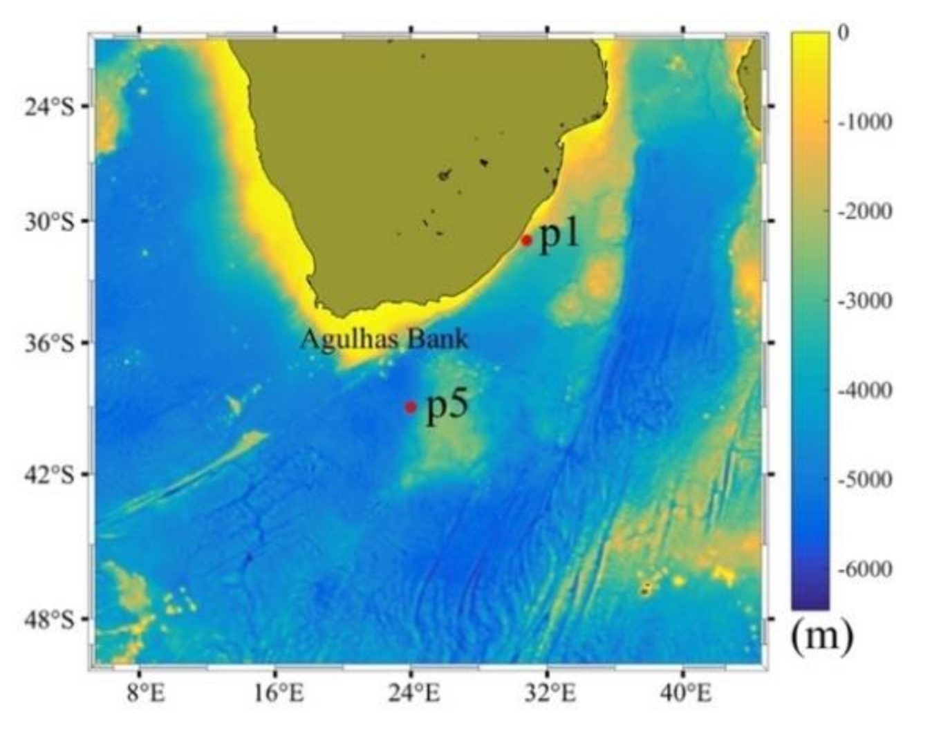
Models such as SWAN are classified as Third Generation Spectral wave models. The configuration of SWAN version 41.31 (Simulating Waves Nearshore) [31,32] grid model covers the AC system region and it extends from 50° S, 19° S up to 5° E, 45° E, at spatial resolution of 0.05°. The bathymetry grid data Etopo1 [33] come from the NOAA’s National Geophysical Data Centre, with a resolution of 1 min of degree in latitude and longitude, which was linearly interpolated to the model grid. Figure 1 shows the bathymetry data and the distribution of the SWAN output locations P1 (31° E, 31° S) and P5 (25° E, 38.36° S).
In this SWAN model configuration, the wave spectrum is provided for 36 directional bands measured clockwise with respect to true north, and 36 frequencies logarithmically spaced from the minimum frequency of 0.030 Hz.
The simulation covers one month from 15 June 2018 up to 15 July 2018 for the integration of the energy balance equation. The integration time step is set at 300 seconds. The wave hindcast wind input and model output time steps were set to 1 hour (Table 1). The wave model was forced with the boundary conditions taken from the ECMWF (European Centre for Medium-Range Weather Forecasts) Era5 reanalysis wave model [34]. For the nested grid shown in Figure 1, the ERA-5 ECMWF wind reanalysis [35] was chosen. More details about the wave model implementation used can be found in Table 1.
ERA5 wind is distributed at 32 km horizontal resolution with 137 vertical levels and at 3-hourly intervals. Analysis fields are prepared hourly with inclusion of newly reprocessed observational data, using the 4D-Var data assimilation technique and the IFS cycle 41r2 model version (operational in 2016). The ERA5 HRES atmospheric data has a resolution of 31km, 0.28125°, and the EDA has a resolution of 62 km, 0.5625°. ERA5 data available from the CDS (Climate Data Store of Copernicus Climate Change service) was pre-interpolated to a regular latitude/longitude grid appropriate for that data.
For the simulation considering currents, current Ocean data from Mercator Ocean in the framework of the Copernicus Marine Environment Monitoring Service (CMEMS) were used. The Operational Mercator global ocean analysis-forecast (phy-0010024) is an hourly product with a 1/12° of horizontal resolution [36]. Mercator Ocean monitoring and forecasting systems have been routinely operated in real time since early 2001. The time series starts on December 26, 2006 until real time [37].
The evolution of the two-dimensional ocean wave spectrum F(f—frequency, θ—mean wave propagation direction, φ—latitude, λ—longitude) with respect to the frequency and direction as a function of latitude and longitude is governed by the transport or balance Equation (1) [38]. The model is formulated in finite differences on regular and rectangular grids. In the presence of currents, the governing equation for deep water can be written as,
where, t is the time, u is the current velocity and Cg is the group velocity at which the information travels along the geographical domain. In deep water, the magnitude of the intrinsic group velocity is Cg = cp/2, where the phase velocity is cp.
To the right hand Stot is the source function which considers all the physical processes that allow the growth and the decay of waves: the wave energy generation, dissipation and nonlinear wave-wave interaction. The main processes included in the SWAN model are wave generation by wind [39], nonlinear resonant wave-wave interactions [40], and the whitecapping [41]. The model also considers the shoaling, the refraction due to depth and the refraction of waves due to ocean currents, the bottom friction and the depth-limited breaking [31].
In the present study, the Benjamin–Feir Index (BFI) is used to characterize the probability of occurrence of extreme waves. BFI is the ratio between non-linearity and dispersion [42]:
where ε = kp(m0)1/2 is the integral steepness parameter (kp is the peak wave number and m0 is the spectral zero moment); Qp is Goda’s parameter (peakedness parameter):
BFI = ε Qp (2π)1/2
F(f) is the 1D frequency spectrum, defined as F(f) = , where F(f,θ) is the 2D frequency-direction wave power spectrum where f is the frequency and is the mean wave propagation direction.
2.2. Validation of the Numerical Simulations
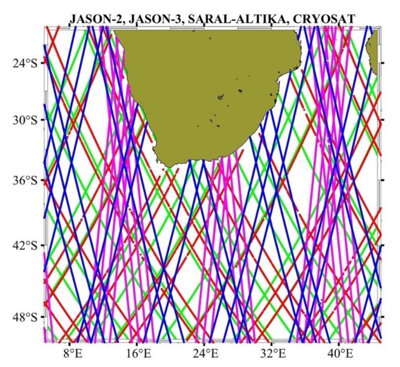
The validation of the two wave hindcasts is done using satellite altimetry data from all the missions that coincided with the simulation period (Figure 2). The validation is performed for the significant wave height (Hs) using the collocation method of satellite altimetry data. The satellite observations are compared to model outputs by averaging the satellite measurements inside a grid cell, around the model output time, and comparing to the average of model output at the grid cell corners.
Table 2 shows some of the statistical parameters computed for each sensor for a week (21–27 June 2018). The validation was made for the two hindcasts performed: (1) considering only waves (WWav) and (2) including currents (WCur). The bias was defined as the difference between the mean observation and the mean prediction. The scatter index (s.i.) is defined as the standard deviation of the predicted data with respect to the best fit line, divided by the mean observations.
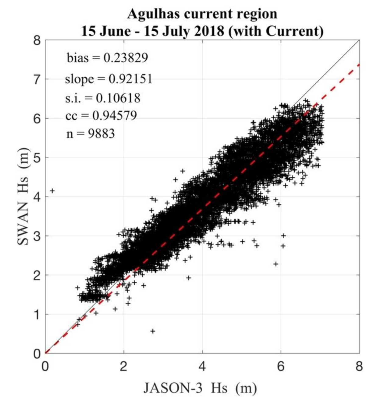
The best correlation coefficient found corresponds to the collocated data of Jason–3 (0.9557, case WCur with current) and the worst value obtained is for Cryosat (0.9207, case WWav only waves). The scatter index varied in the range of 0.1020 (SARAL–ALtika, WCur) to 0.1502 (Jason–3, WWav), the bias obtained varied from 0.2303 (Cryosat, WCur) to −0.6025 (Cryosat, WWav). The best slope corresponds to Jason–3 with 0.9215 (Figure 3) (WCur) and the highest value corresponds to Jason–3 (1.1351, WWav) (Table 2). The lowest RMSE is obtained from the collocation of the Hs between Cryosat and SWAN from the simulation WCur with 0.5387 and the highest resulted from Jason–3 WWav 0.8142.
As can be seen, although the systematic deviation (bias) seems to be slightly higher for the case with currents, the absolute errors, as measured by the RMS error is lower for the simulation with currents, which also improves the dispersion (s.i) and the correlation coefficient between the hindcast and satellite measurements.
2.3. ESA Sentinel-1 SAR Wave Mode Data
Since the launch of Sentinel-1 satellites in 2014, innumerable investigations using S1 SAR imagery have been developed [43,44,45]. The SAR provides ocean wave and surface wind information on an uninterrupted way and at global scale.
The Ocean Swell Spectra (OSW) component is a 2-dimensional ocean surface swell spectrum and contains an estimate of the wind speed and direction per swell spectrum. The OSW component provides continuity measurement of SAR swell spectra at C-band. OSW are estimated from Sentinel-1 Single Look Complex (SLC) images by inversion of the corresponding image cross-spectra [46].
The OSW is generated from Stripmap and Wave modes only and is not available from the TOPSAR IW (Interferometric Processing Facility) and Extra-Wide Swath (EW) modes. For Stripmap mode, there are multiple spectra derived from the Level-1 SLC image. For Wave mode, there is one spectrum per vignette [47,48].
Wave mode products consist of several vignettes with each vignette processed as a separate image. The wave mode acquires data in 20 km by 20 km vignettes, every 100 km along the orbit, acquired alternately on two different incidence angles. One half of the vignette is acquired with one incidence angle and the other half is acquired with another incidence angle [49].
Ocean wave height spectra are provided in units of m4 and given on a polar grid of wavenumber in rad/m and direction in degrees with respect to North.
3. Results and Discussions
3.1. Winter Synoptic Conditions
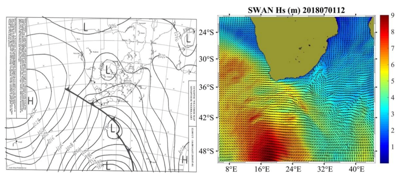
During the winter months (May to October) severe storms are common in the Agulhas Current region. According to South African Weather Service synoptic chart, on the 30 June 2018, a deep depression (976 hPa) and the associated cold front located at 47.8° S and 16° E were observed traversing quickly the area of study from West to East on 1 July 2018 (984 hPa). Figure 4 (left) shows the synoptic conditions for the 1 July2018.
The fetch and strength of the southwesterly winds develop moderate swell (periods of about 15 s and wavelength of 200 m) with high wave heights reaching the South African coast and pushing the bulk of the wave energy towards the region of the Agulhas Current system. The fetch of the southwesterly winds blowing across the Southern Ocean, is of thousand miles and consequently the Hs shows a maximum of 9 m (Figure 4, right).
3.2. Temporal Analysis
In this section the temporal variability of the main wind and ocean current parameters is analyzed at two locations AC (at P1) and in the ACR (at P5), together with the standard averaged wave parameters retrieved from SWAN.
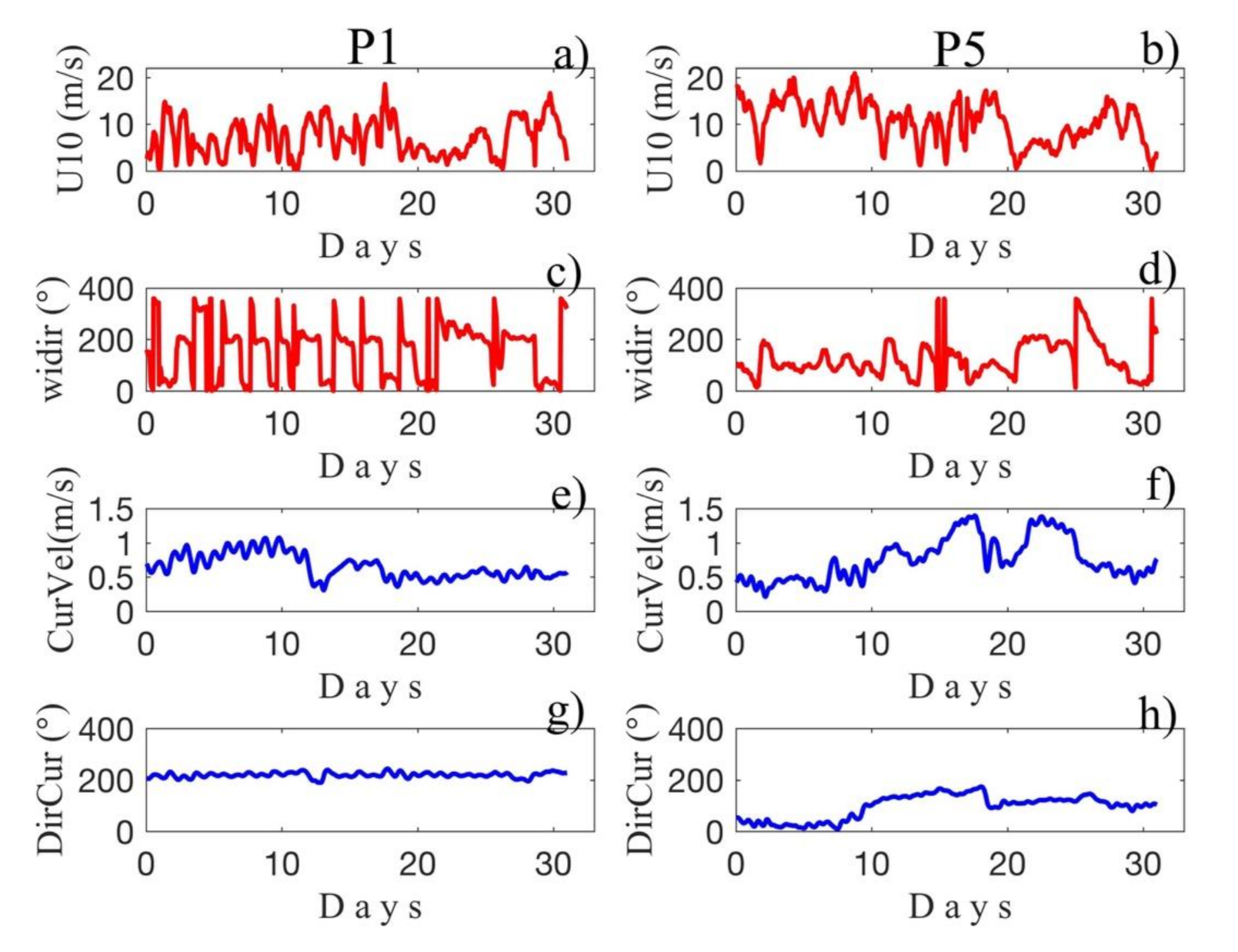
Along the simulation period (15 June 2018–15 July 2018) windspeed at P1 is lower than at P5 (Figure 5a,b). At P1, only 26% of the time is the wind speed above 10 m/s while at P5 this fraction is 58%. Wind direction at P1 is predominantly alongshore (either NE or SW), while at P5 the wind blows consistently from the West as a result of Antarctic Circumpolar jet. Currents at P1 (Figure 5e,g) are dominated by the southward flowing alongshore Agulhas Current that rarely exceeds 1 m/s (4% of the time). At P5, the circulation is dominated by the meandering of the Agulhas Retroflection. Here, current velocities above 1 m/s occur 23% of the time and the flow is either southwestward or northeastward, which puts P5 in the center of the almost stationary first Agulhas Retroflection meander, when the current changes direction and flows into the Indian Ocean.
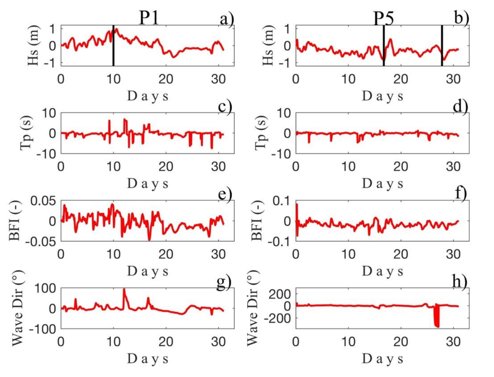
At P1 the ΔHs is positive until day 20 (Figure 6). From day 5 it increases until reaching a maximum of approximately 1 m on day 10. From this day onward until day 20 steadily decreases and from day 20 until the end of the simulation the ΔHs is slightly negative.
During this period, variations in wind speed and directions occur at a much faster time scale, so the increase in Hs when using currents should not be related to wind effect on waves or currents.
Rather, the increase in Hs from day 5 to day 10 seems to be due to a blocking effect of the current on the waves because during this period currents and waves flow in opposing directions and we observe a simultaneous increase in current velocity. From day 10 to day 14 the current velocity decreases to 0.5 m/s and remains around this value for the rest of the simulation.
During this period when the wave blocking by current takes place, changes in the peak period (Tp) due to currents are not observed, the BFI differences fluctuate much faster than the blocking and only a slight trend following the increase of Hs maybe perceived in the time series.
At P5, differences in Tp are also trendless (Figure 6). Here, Hs differences are consistently negative: −0.31 m on average, while at P1 the average ΔHs is 0.07 m. A negative trend is observed in ΔHs at P5 from the beginning of the simulation until approximately day 15. From this day onward, ΔHs is slightly negative but steady. The Hs decrease when currents are present during the first half of the simulation appears to be a result of the change in current velocity and heading in the fixed position of P5 due to the passage of a meander. During this period, the current velocity increases from 0.5 m/s to nearly 1 m/s and the current heading changes from the NW to the SW and then South. With reference to the wave direction, which remains steadily eastward during this period, the current goes from crossing to following and to crossing again, so the decrease in Hs must be caused by the stretch of the meander where the current flows eastward with the waves.
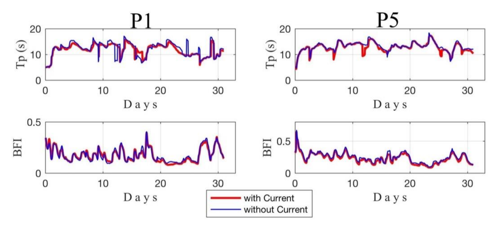
In addition, it was observed that, after the decrease of the peak period, the BFI reached the maximum value. In general, at location P1 and P5 the high values of BFI observed are in a direct relation with a decrease of the Tp (Figure 7) as reported earlier in other studies [50,51,52].
The formulation for the BFI that the wave model used does not have any directionality information and is based on a balance between nonlinearity and dispersion for narrow banded sea state. The directionality of the sea state is introduced in the calculation of the Kurtosis that is the statistical measure of the probability of occurrence of extreme waves.
The model uses a quasi-linear dissipation source function that considers the square of the mean steepness which was reformulated in terms of a mean steepness parameter and a mean frequency, giving more emphasis on the high-frequency part of the spectrum and results in a more realistic interaction between wind sea and swell.
3.3. Composite Spatial Analysis of the Extreme Waves
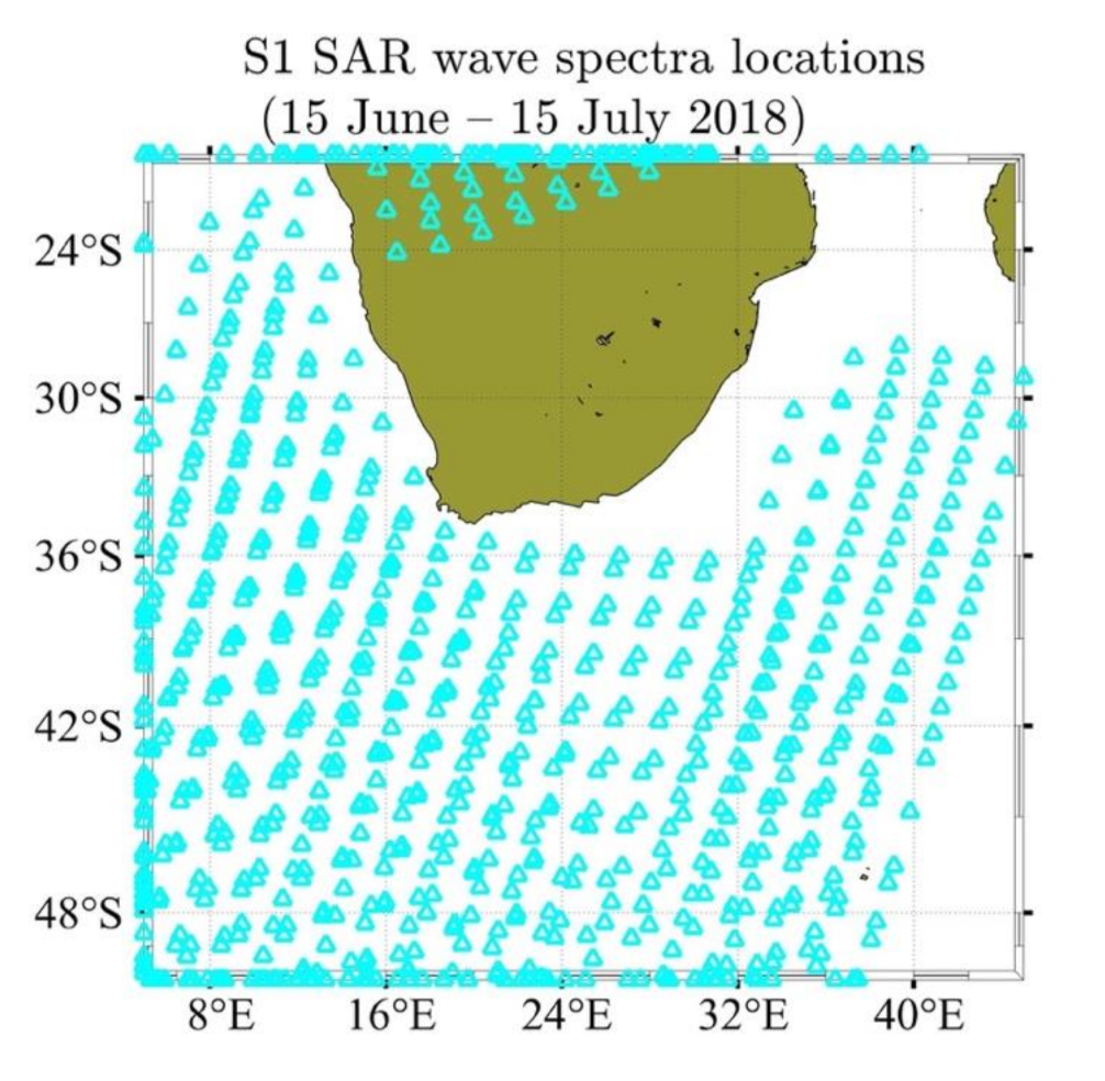
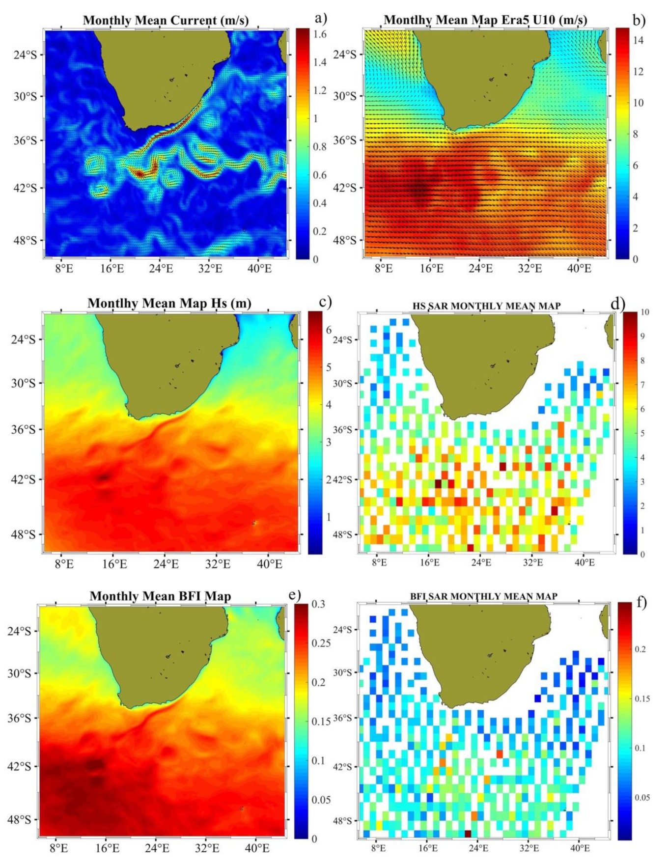
In this section, the monthly composites of Hs and BFI are analyzed. The comparison of the spatial distribution is between the data measured by SAR and the model results. The distribution of the SAR data is depicted in Figure 8 showing a good coverage of the region of study. The monthly mean map of the AC shows that the higher values are around 1.6 m/s distributed mainly in the Northern AC and in the ARC (Figure 9a). In addition, eddies are less intense in terms of current velocity with speeds of about 1 m/s. The current mean map was computed using the MERCATOR ocean data for the period of 15 June 2018–15 July 2018.
The Hs monthly composite (Figure 9c) shows that the model captured the AC and the ACR features as can be seen with maximum values of 5–6 m in those places where the current is intense both in the mainstream and in the meanders and eddies (Figure 9a). Whereas, the Hs composite constructed with the SAR data (Figure 9d) show a similar pattern with the maxima values distributed in the ACR where strong wave-current interactions take place together with the focusing. Unfortunately, the Sentinel 1 SAR instrument did not pass in the region of the Agulhas Current (Northern part) as can be seen from Figure 8. The other region where Hs maximum values were observed by SAR was especially in the southern limit of the domain that is affected by the strong westerly circumpolar winds around Antarctic (Figure 9b).
In the Southern Ocean it has been reported that the reduction of the mean wave energy in presence of currents is mainly due to the relative wind effect in a global scale, except where strong local currents occur. The Antarctic Circumpolar Current plays a key role in reducing the momentum transfer from the wind to the waves [30].
In general, a direct correlation was found between the modelled Hs and the Hs SAR data patterns.
In the case of the BFI, the comparison between the modeled and observed composites (Figure 9e,f) exhibits the highest values located in the ACR and a few high values are observed in the southern border, as occurred with the Hs. A remark can be done emphasizing the fact that the numerical simulations are very useful since they can provide information in those places where the satellite instrument lacks as happens in this case with the AC (Northern part was not observed by SAR, Figure 8). The modeled monthly composite of BFI shows that the highest values are located in the AC and in the ACR. It is necessary to point out that the BFI did not result too high as to say that we found freak waves, but the results of this study indicate that there is direct correlation between the Agulhas Current intensity and the Hs and BFI.
4. Analysis of the Wave Spectra
4.1. Influence of Currents on the Modelled 2d Wave Spectra
This section presents a comparison between the 2d wave spectra from the simulations with and without current at two locations: P1 and P5 located in quite different places since the North part of the AC (P1) is more stable than the ACR (P5) (Figure 9a) where the current fluctuates, having a meandering character with different current directions and deflections that could have some effects on the wave field and consequently in the spectral shapes.
Wave spectra often have one swell component and one wind sea condition, which are combined to represent what is denoted as the total wave spectra [53]. The concept is also adopted when more sea components are present [54].
From the obtained results it can be seen that the intensity of the current is very important and modifies the wave spectrum in a noticeable manner. In addition, the attention was focused on the wave and current directions. Three different situations are analyzed below.
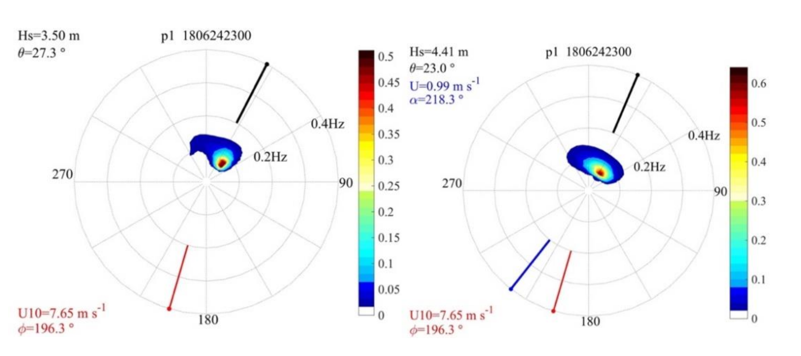
4.2. Case 1: Waves in Opposing Current (P1)
Wave spectra were retrieved from SWAN at P1 (Figure 1) for the date 24 June 2016 at 23 UTC, when the current speed (0.99 m/s) from the NE (blue arrow in Figure 10) as well as the wind direction (from NE red arrow), whereas waves propagate against the current and the wind from the SW direction (black arrow). The effect of the current on the spectrum is therefore to broaden as can be observed and to grow the spectral wave energy.
The analysis of the wave spectra evolution at P1, showed that in general if the current velocity is about 1 m/s and the wave and current propagate in opposing directions (aligned), an increase in the spectral wave energy occurs.
The Hs is higher (4.41 m, Figure 10, right panel) from the simulation with current in contrast with the wave spectrum from (Figure 10, left panel, no current) where the level of the spectral wave energy is inferior. In particular, the difference between the Hs (with and without current cases) was 91 cm.
In the region of the ACR, which is a region with a noticeable variability due to the meandering, the modeled wave spectra resulted quite different that those obtained inP1.
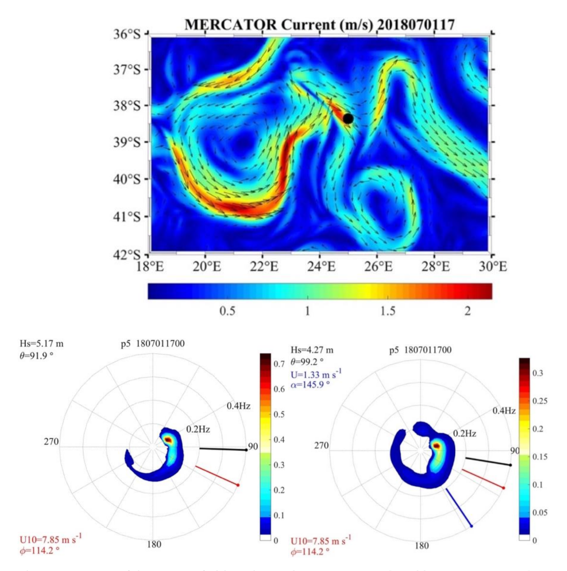
4.3. Case 2: Waves and Current Not Aligned (P5)
The complexity of the spectra is shown in Figure 11 and Figure 12. Two different dates are analyzed at P5 (coordinates −38.36° S, 25° E. Figure 1) without and with current, respectively, on the 1 July 2018 at 17 UTC and 12 July 2018 at 19 UTC.
From these spectra (01/07/2018 at 17 UTC, Figure 11) it is possible to see how in presence of a strong current (velocity = 1.33 m/s) the wave spectrum is transformed due to the wave refraction induced by the current. In this case the wave energy decreased (Figure 11 bottom panel). As can be seen the Hs in the wave spectrum (simulation without current (left panel)) is higher than the spectrum from the right panel (simulation with current (right panel)). In this case the difference between the Hs from the simulation considering current and without current was 90 cm. This is the largest difference in Hs found at P5 and occurs when a meander crosses P5 flowing to SE (Figure 11, top panel). In this situation, although the waves and current are separated by 45 degrees, the current speed is high enough (1.33 m/s) to cause a decrease in Hs. In addition, the spectral energy (with current considered) covers almost whole the circle as the wave and current are not aligned.
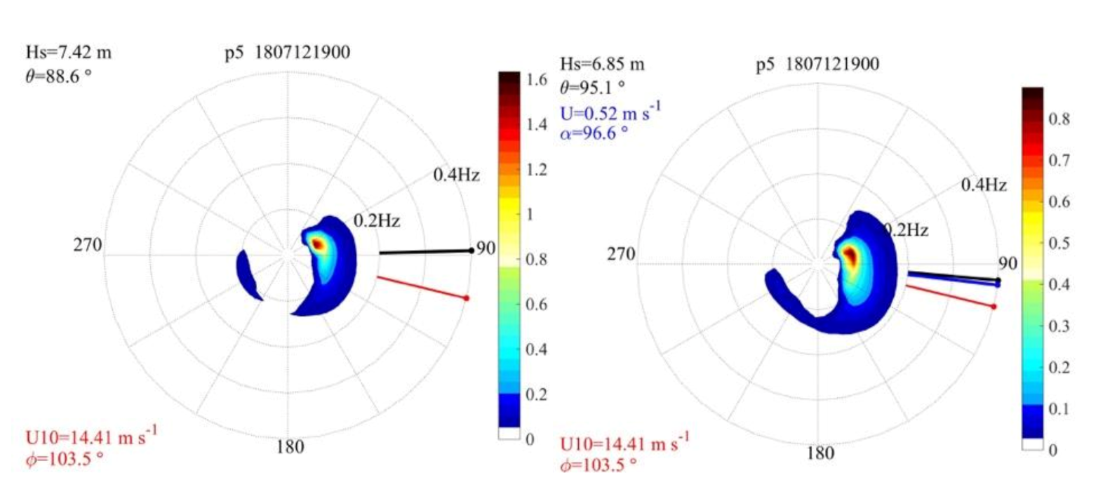
4.4. Case 3: Waves in a Following Current (P5)
As can be seen, when wave and current are aligned (12 July 2018 at 19 UTC, Figure 12) the effect is the opposite: the spectral wave energy decreases, and the shape of the wave spectrum lengthens and broadens as reported in [55,56]. When currents are included (right panel) in the simulations the Hs decreases 0.57 m with respect to the simulation without currents. In presence of currents, the decrease of wave energy was also reported in [30]. If winds and currents are running in the same direction, the momentum flux to the waves is reduced and the resultant waves are smaller. Instead, if waves and currents are opposed, the wind stress increases and so does the momentum flux from wind to waves.
5. Conclusions
The obtained results demonstrate that in the presence of a strong current (of the order of 1.38 m/s) the wave spectrum suffers a transformation due to wave-current interaction. However, in the present study the nonlinear mechanisms that might have generated extreme waves are not discussed because the SWAN model is a phase-averaged model.
The explicit representation of abnormal waves in the spectrum of waves is not possible as only statements about the probability of occurrence of individual waves can be related to spectral parameters. The present study uses the standard extreme wave parameter BFI computed by the SWAN model to get more information about dangerous waves in the Agulhas Current Retroflection region and nearby the coast where an intense maritime traffic takes place. The high values depicted in the ACR are located in the zones where waves experienced rapid changes due to the interaction with this strong ocean current.
The wave-current interaction and the focusing due to the current in the Agulhas Current Retroflection result in many peaked wave spectra if the wave and the current are in an opposite direction (aligned or almost aligned), as was shown in the present study inferred from high resolution numerical simulations.
In the Agulhas Current Retroflection region, the modelled wave spectra are broader than those obtained from simulations without currents. Similar spectral shapes have been reported in [54]. Results obtained in present work must be taken with caution since the present spatial resolution of the oceanic current data used (MERCATOR) does not fully resolve the mesoscale vorticity and for this reason the simulation considering ocean currents may likely underestimate the effects of currents on waves.
The exclusion of oceanic current in a simulation, in regions of strong currents such as the Agulhas Current system could lead to a wrong prediction of the extreme wave parameters and consequently to an unrealistic extreme sea states which is essential for the maritime activities and safety. In addition, when surface currents are taken into account in the model, a significant improvement is seen in the modeled wave parameters.
The current effects basically produce blocking, whirling and bunching. It remains to be fully understood why spectral models cannot fully deal with the special circumstances such as rapid changes in the flow of intense currents such as the Gulf Stream, Agulhas or Kuroshio. Correctly reproducing the refraction produced by this kind of currents in the swell through numerical simulations mainly requires that the current gradients be sufficiently exact as input data to the high resolution (not only in time and space, but also in the spectral domain) wave models. Even so, having the best existing ocean current product to date, the physics of the wave model will present limitations.
In the future, we plan to continue this investigation using high resolution coupled wave-current simulations able to represent better the current gradients and sub-mesoscale vorticity.
Author Contributions
S.P.d.L.: Conceptualization; methodology; validation; formal analysis; writing—original draft, review and editing; C.G.S.: writing—review and editing. All authors have read and agreed to the published version of the manuscript.
Funding
This work contributes to the Strategic Research Plan of the Centre for Marine Technology and Ocean Engineering (CENTEC), which is financed by the Portuguese Foundation for Science and Technology (Fundação para a Ciência e Tecnologia—FCT) under UIDB/UIDP/00134/2020. The first author has been contracted as a Researcher funded by FCT through Scientific Employment Stimulus.
Data Availability Statement
The data presented in this study are not publicly available because the data is still being used for follow-up studies.
Acknowledgments
The first author is grateful to the European Space Agency for the training on Sentinel SAR data provided during the “25 Years of Progress in Radar Altimetry” Symposium, São Miguel, Azores.
Conflicts of Interest
The authors declare no conflict of interest.
References
- Guedes Soares, C.; Teixeira, A.P. Risk assessment in maritime transportation. Reliab. Eng. Syst. Saf. 2001, 74, 299–309. [Google Scholar] [CrossRef]
- Guedes Soares, C.; Bitner-Gregersen, E.; Antao, P. Analysis of the Frequency of Ship Accidents under Severe North Atlantic Weather Conditions. In Proceedings of the Conference on Design and Operation for Freak Conditions II, Royal Institution of Naval Architects (RINA), London, UK, 6–7 November 2001; pp. 221–230. [Google Scholar]
- Vettor, R.; Guedes Soares, C. Development of a ship routing system. Ocean Eng. 2016, 123, 1–14. [Google Scholar] [CrossRef]
- Draper, L. “Freak” ocean waves. Weather 1966, 21, 2–4. [Google Scholar] [CrossRef]
- Dean, R.G. Freak waves: A possible explanation. In Water Wave Kinetics; Tørum, A., Gudmestad, O.T., Eds.; (NATO ASI Series (E Applied Sciences)); Springer: Dordrecht, The Netherlands, 1990; Volume 178. [Google Scholar] [CrossRef]
- Fedele, F.; Brennan, J.; de León, S.P.; Dudley, J.; Dias, F. Real world ocean freak waves explained without the modulational instability. Sci. Rep. 2016, 6, 27715. [Google Scholar] [CrossRef] [PubMed]
- Dudley, J.M.; Genty, G.; Mussot, A.; Chabchoub, A.; Dias, F. Rogue waves and analogies in optics and oceanography. Nat. Rev. Phys. 2019, 1, 675–689. [Google Scholar] [CrossRef]
- Lavrenov, I. The wave energy concentration at the Agulhas current of South Africa. Nat. Hazards 1998, 17, 117–127. [Google Scholar] [CrossRef]
- Tamura, H.; Waseda, T.; Miyazawa, Y. Freakish sea state and swell-windsea coupling: Numerical study of the Suwa-Maru incident. Geophys. Res. Lett. 2009, 36, L01607. [Google Scholar] [CrossRef] [Green Version]
- Cavaleri, L.; Bertotti, L.; Torrisi, L.; Bitner-Gregersen, E.; Serio, M.; Onorato, M. Rogue waves in crossing seas: The Louis Majesty accident. J. Geophys. Res. 2012, 117, C00J10. [Google Scholar] [CrossRef]
- Waseda, T.; In, K.; Kiyomatsu, K.; Tamura, H.; Miyazawa, Y.; Iyama, K. Predicting freakish sea state with an operational third-generation wave model. Nat. Hazards Earth Syst. Sci. 2014, 14, 945–957. [Google Scholar] [CrossRef] [Green Version]
- Ponce de León, S.; Bettencourt, J.H.; Brennan, J.; Dias, F. Evolution of the Extreme Wave Region in the North Atlantic Using a 23 Year Hindcast. In Proceedings of the ASME. International Conference on Offshore Mechanics and Arctic Engineering, Volume 2: Structures, Safety and Reliability (OMAE2015):V003T02A019, Newfoundland, NL, Canada, 31 May–5 June 2015. [Google Scholar] [CrossRef]
- Ponce de León, S.; Bettencourt, J.H.; Dias, F. Comparison of hindcasted extreme waves with a Doppler radar measurements in the North Sea. Ocean Dyn. 2017, 67, 103–115. [Google Scholar] [CrossRef]
- Mallory, J.K. Freak waves in the south-east coast of South Africa. Int. Hydrogr. Rev. 1974, 51, 99–129. [Google Scholar]
- Gründlingh, M.L. TOPEX/Poseidon observes wave enhancement in the Agulhas current. AVISO Altimeter Newsl. 1994, 3. [Google Scholar]
- Krug, M.; Swart, S.; Gula, J. Submesoscale cyclones in the Agulhas current. Geophys. Res. Lett. 2017, 44, 1–9. [Google Scholar] [CrossRef] [Green Version]
- Lutjeharms, J.R.E. The Agulhas Current; Springer: Berlin, Germany; New York, NY, USA, 2006; Available online: https://0-link-springer-com.brum.beds.ac.uk/content/pdf/10.1007/3-540-37212-1.pdf (accessed on 10 March 2019)ISBN 10 3-540-42392-3.
- Johannessen, J.A.; Chapron, B.; Collard, F.; Kudryavtsev, V.; Mouche, A.; Akimov, D.; Dagestad, K.F. Direct ocean surface velocity measurements from space: Improved quantitative interpretation of Envisat ASAR observations. Geophys. Res. Lett. 2008, 35, L22608. [Google Scholar] [CrossRef] [Green Version]
- Rouault, M.J.; Mouche, A.; Collard, F.; Johannessen, J.A.; Chapron, B. Mapping the Agulhas current from space: An assessment of ASAR surface current velocities. J. Geophys. Res. 2010, 115, C10026. [Google Scholar] [CrossRef] [Green Version]
- Krug, M.; Tournadre, J.; Dufois, F. Interactions between the Agulhas Current and the eastern margin of the Agulhas Bank. Cont. Shelf Res. 2014, 81, 67–79. Available online: https://0-www-sciencedirect-com.brum.beds.ac.uk/science/article/pii/S0278434314000843 (accessed on 15 April 2020). [CrossRef] [Green Version]
- Bang, N.D. Dynamic interpretations of a de- tailed surface temperature chart of the Agulhas Current retroflexion and fragmentation area. S. Afr. Geogr. J. 1970, 52, 67–76. [Google Scholar] [CrossRef]
- Lutjeharms, J.R.E.; van Ballegooyen, R.C. The retroflection of the Agulhas Current. J. Phys. Oceanogr. 1988, 18, 1570–1583. [Google Scholar] [CrossRef]
- Lutjeharms, J.R.E. Features of the southern Agulhas Current circulation from satellite remote sensing. S. Afr. J. Sci. 1981, 77, 231–236. Available online: https://journals.co.za/content/sajsci/77/5/AJA00382353_1526 (accessed on 3 January 2018).
- Broecker, W.S. The great ocean conveyor. Oceanography 1991, 4, 79–89. [Google Scholar] [CrossRef]
- Johannessen, J.A.; Chapron, B.; Collard, F.; Backeberg, B. Use of SAR Data to Monitor the Greater Agulhas Current. In Remote Sensing of the African Seas; Barale, V., Gade, M., Eds.; Springer: Cham, Switzerland, 2014; ISBN 978-94-017-8007-0. [Google Scholar] [CrossRef]
- Young, I.R.; Ribal, A. Multiplatform evaluation of global trends in wind speed and wave height. Science 2019, 364, 548–552. [Google Scholar] [CrossRef]
- Young, I.R.; Zieger, S.; Babanin, A. Global trends in wind speed and wave height. Science 2011, 332, 451–455. [Google Scholar] [CrossRef] [PubMed]
- Quilfen, Y.; Yurovskaya, M.; Chapron, B.; Ardhuin, F. Storm waves focusing and steepening in the Agulhas current: Satellite observations and modeling. Remote Sens. Environ. 2018, 216, 561–571. [Google Scholar] [CrossRef] [Green Version]
- Ardhuin, F.; Gille, S.T.; Menemenlis, D.; Rocha, C.B.; Rascle, N.; Chapron, B.; Gula, J.; Molemaker, J. Small-scale open-ocean currents have large effects on wind- wave heights. J. Geophys. Res. Oceans 2017, 122, 4500–4517. [Google Scholar] [CrossRef] [Green Version]
- Rapizo, H.; Durrant, T.H.; Babanin, A.V. An assessment of the impact of surface currents on wave modeling in the Southern Ocean. Ocean Dyn. 2018, 68, 939–955. [Google Scholar] [CrossRef]
- Booij, N.; Ris, R.C.; Holthuijsen, L.H. A third-generation wave model for coastal regions. 1. Model description and validation. J. Geophys. Res. 1999, 104, 7649–7666. [Google Scholar] [CrossRef] [Green Version]
- SWAN Team. SWAN Scientific and Technical Documentation; Delft University of Technology: Delft, The Netherlands, 2019. [Google Scholar]
- Amante, C.; Eakins, B.W. ETOPO1 1 Arc-Minute Global Relief Model: Procedures, Data Sources and Analysis; NOAA Technical Memorandum NESDIS NGDC-24; National Geophysical Data Center NOAA: Boulder, CO, USA, 2009. [Google Scholar] [CrossRef]
- IFS Documentation-Cy46r1. Operational Implementation, 6 June 2019. Part VII: ECMWF Wave Model; European Centre for Medium-Range Weather Forecasts: Shinfield Park, Reading, UK; p. 99. Available online: https://www.ecmwf.int/sites/default/files/elibrary/2019/Part-VII-ECMWF-Wave-Model.pdf (accessed on 2 February 2021).
- Hersbach, H.; Bell, W.; Berrisford, P.; Horányi, A.; Muñoz-Sabater, J.; Nicolas, J.; Radu, R.; Schepers, D.; Simmons, A.; Soci, C.; et al. Global Reanalysis: Goodbye ERA-Interim, Hello ERA5; ECMWF Newsletter: Reading, UK, 2019; pp. 17–24. [Google Scholar] [CrossRef]
- Lellouche, J.-M.; Greiner, E.; Le Galloudec, O.; Garric, G.; Regnier, C.; Drevillon, M.; Benkiran, M.; Testut, C.-E.; Bourdalle-Badie, R.; Gasparin, F.; et al. Recent updates to the Copernicus Marine Service global ocean monitoring and forecasting real-time 1∕12°high-resolution system. Ocean Sci. 2018, 14, 1093–1126, Copernicus Publications. [Google Scholar] [CrossRef] [Green Version]
- Law Chune, S.; Nouel, L.; Fernandez, E.; Derval, C. Product User Manual for the Global Ocean Sea Physical Analysis and Forecasting Products; CMEMS: Brussels, Belgium, 2019; 30p, Available online: http://marine.copernicus.eu/services-portfolio/access-to-products/?option=com_csw&view=details&product_id=GLOBAL_ANALYSIS_FORECAST_PHY_001_024 (accessed on 2 February 2021).
- Komen, G.J.; Cavaleri, L.; Donelan, M.A.; Hasselmann, K.; Hasselmann, S.; Janssen, P.A.E.M. Dynamics and Modelling of Ocean Waves; Cambridge University Press: Cambridge, UK, 1994; Available online: https://0-www-cambridge-org.brum.beds.ac.uk/core/books/dynamics-and-modelling-of-ocean-waves/767155B50D6E29B0F62729F29C2DE124 (accessed on 2 February 2021).
- Komen, G.J.; Hasselmann, S.; Hasselmann, K. On the existence of a fully developed wind-sea spectrum. J. Phys. Oceanogr. 1984, 14, 1271–1285. [Google Scholar] [CrossRef]
- Hasselmann, S.; Hasselmann, K.; Allender, J.H.; Barnett, T.P. Computations and parameterizations of the nonlinear energy transfer in a gravity-wave spectrum, Part II. J. Phys. Oceanogr. 1985, 15, 1378–1391. [Google Scholar] [CrossRef] [Green Version]
- Janssen, P.A.E.M. Quasi-linear theory of wind wave generation applied to wave forecasting. J. Phys. Oceanogr. 1991, 21, 1631–1642. [Google Scholar] [CrossRef] [Green Version]
- Janssen, P.A.E.M. Nonlinear four-wave interactions and freak waves. J. Phys. Oceanogr. 2003, 33, 863–884. [Google Scholar] [CrossRef]
- Ardhuin, F.; Stopa, J.; Chapron, B.; Collard, F.; Smith, M.; Thomson, J.; Doble, M. Measuring Ocean Waves in Sea Ice Using SAR Imagery: A Quasi-Deterministic Approach Evaluated with Sentinel-1 and in Situ Data. Remote Sens. Environ. 2016, 189, 211–222. [Google Scholar] [CrossRef] [Green Version]
- Stopa, J.E.; Mouche, A. Significant wave heights from Sentinel-1 SAR: Validation and applications. J. Geophys. Res. Oceans 2017, 122, 1827–1848. [Google Scholar] [CrossRef] [Green Version]
- Rikka, S.; Pleskachevsky, A.; Jacobsen, S.; Alari, V.; Uiboupin, R. Meteo-marine parameters from Sentinel-1 SAR imagery: Towards near real-time services for the baltic sea. Remote Sens. 2018, 10, 757. [Google Scholar] [CrossRef] [Green Version]
- Johnsen, H.; Collard, F. Sentinel-1 Ocean Swell Wave spectra (OSW) Algorithm Definition NORUT Report 13/2009; NORUT: Narvik, Norway; ISBN 1890-5226. Available online: https://earth.esa.int/documents/247904/349449/S-1_L2_OSW_Detailed_Algorithm_Definition.pdf (accessed on 2 February 2021).
- Collard, F.; Chapron, B.; Johnsen, H. Sentinel-1 SAR Wave Mode, Technical Note, Boost Technologies, v1.0, Dec 2007. Available online: https://sentinel.esa.int/documents/247904/349449/S1_L2_OSW_Detailed_Algorithm_Definition.pdf (accessed on 2 February 2021).
- European Space Agency. Sentinel-1 User Handbook 2015; ESA: Paris, France; 64p, Standard Document, Issue 1, Rev. 2; Available online: https://sentinel.esa.int/documents/247904/685211/Sentinel-2_User_Handbook (accessed on 2 February 2021).
- Attema, E.; Cafforio, C.; Gottwald, M.; Guccione, P.; Guarnieri, A.M.; Rocca, F. Flexible dynamic block adaptive quantization for Sentinel-1 SAR missions. IEEE Geosci. Remote Sens. Lett. 2010, 7, 766–770. [Google Scholar] [CrossRef]
- Osborne, A.R.; Ponce de León, S. Properties of Rogue Waves and the Shape of the Ocean Wave Power Spectrum. In Proceedings of the ASME 36th International Conference on Offshore Mechanics and Arctic Engineering, Volume 3A: Structures, Safety and Reliability:V03AT02A013, Trondheim, Norway, 25–30 June 2017. [Google Scholar] [CrossRef]
- Ponce de León, S.; Osborne, A.; Guedes Soares, C. On the importance of the exact nonlinear interactions in the spectral characterization of rogue waves. In Proceedings of the 37th International Conference on Ocean, Offshore and Arctic Engineering, OMAE2018, Madrid, Spain, 17–22 June 2018. [Google Scholar] [CrossRef]
- Ponce de León, S.; Osborne, A.R. Role of Nonlinear Four-Wave Interactions Source Term on the Spectral Shape. J. Mar. Sci. Eng. 2020, 8, 251. [Google Scholar] [CrossRef] [Green Version]
- Guedes Soares, C. Representation of Double-Peaked Sea Wave Spectra. Ocean Eng. 1984, 11, 185–207. [Google Scholar] [CrossRef]
- Boukhanovsky, A.; Guedes Soares, C. Modelling of Multipeaked Directional Wave Spectra. Appl. Ocean Res. 2009, 31, 132–141. [Google Scholar] [CrossRef]
- Kudryavtsev, V.; Yurovskaya, M.; Chapron, B.; Collard, F.; Donlon, C. Sun glitter imagery of surface waves. Part 2: Waves transformation on ocean currents. J. Geophys. Res. Oceans 2017, 122, 1384–1399. [Google Scholar] [CrossRef]
- Ponce de León, S.; Guedes Soares, C. Numerical Modelling of the Effects of the Gulf Stream on the Wave Characteristics. J. Mar. Sci. Eng. 2021, 9, 42. [Google Scholar] [CrossRef]
Figure 1.
Bathymetry grid and locations of the SWAN outputs. P1 (31° E, −31° S) located in the Agulhas Current (AC) and P5 (−38.36° S, 25° E) located in the Agulhas Current Retroflection (ACR) zone.
Figure 1.
Bathymetry grid and locations of the SWAN outputs. P1 (31° E, −31° S) located in the Agulhas Current (AC) and P5 (−38.36° S, 25° E) located in the Agulhas Current Retroflection (ACR) zone.

Figure 2.
Orbit segments of Jason–3 (green), Jason–2 (red), Saral–Altika (blue) and Cryosat (magenta).
Figure 2.
Orbit segments of Jason–3 (green), Jason–2 (red), Saral–Altika (blue) and Cryosat (magenta).

Figure 3.
Scatter plot after the collocation of the SWAN model Hs (considering currents) to the altimeter Hs for a six-day period (21 June 2018–27 June 2018).
Figure 3.
Scatter plot after the collocation of the SWAN model Hs (considering currents) to the altimeter Hs for a six-day period (21 June 2018–27 June 2018).

Figure 4.
The synoptic map showing the weather conditions (left) for the 1 July 2018 at 12 UTC. Right image is the Simulating Waves Nearshore (SWAN) model.
Figure 4.
The synoptic map showing the weather conditions (left) for the 1 July 2018 at 12 UTC. Right image is the Simulating Waves Nearshore (SWAN) model.

Figure 5.
Time series for the Wind speed (a,b), Wind Direction (c,d), Current speed (e,f), Current direction (g,h) at P1 (left) and at P5 (right). Simulation period: 15 June 2018–15 July 2018.
Figure 5.
Time series for the Wind speed (a,b), Wind Direction (c,d), Current speed (e,f), Current direction (g,h) at P1 (left) and at P5 (right). Simulation period: 15 June 2018–15 July 2018.

Figure 6.
Differences (WCur-WWav) between the different averaged wave parameters. Left (at P1), Right (P5): Hs (a,b); Peak Period Tp (c,d); BFI (e,f); Mean wave propagation direction (g,h). Simulation period: 15 June 2018–15 July 2018. Vertical black lines indicate the date where the 2d wave spectra are analyzed in Section 4. (WWav) considering only waves and considering waves and currents (WCur).

Figure 7.
Evolution of the Peak Period (Tp) and BFI at P1 and P5 showing the decrease of the Tp some hours before the increase of the BFI.
Figure 7.
Evolution of the Peak Period (Tp) and BFI at P1 and P5 showing the decrease of the Tp some hours before the increase of the BFI.

Figure 8.
Distribution of the Sentinel 1 (S1) SAR wave mode data.

Figure 9.
Monthly composite map of the ocean current (a), monthly mean wind (b), Modeled Hs monthly composite map (c)(from the simulation considering currents) and SAR observations monthly mean of Hs (d), BFI composite map from the wave model (e) and the computed from SAR mean BFI (f).
Figure 9.
Monthly composite map of the ocean current (a), monthly mean wind (b), Modeled Hs monthly composite map (c)(from the simulation considering currents) and SAR observations monthly mean of Hs (d), BFI composite map from the wave model (e) and the computed from SAR mean BFI (f).

Figure 10.
SWAN wave spectrum at P1 (31° E, 31° S) from the simulation considering only waves (left), affected by the current wave spectrum (right) (Velocity Current = 0.85 m/s) for the 24 June 2018 at 23 UTC. Symbols: φ (wind direction), θ (wave direction), α (current direction), U (Current velocity). The arrowhead (circle) points to where the waves and currents propagate (oceanographic convention).

Figure 11.
Zoom of the current field on the 1 July 2018 at 17 UTC and location P5 (top). SWAN wave spectra at P5 (25° E, 38.36° S) from the simulation considering only waves (left) and considering waves and currents (right). Symbols: φ (wind direction), θ (wave direction), α (current direction), U (Current velocity). The arrowhead (circle) points to where the waves and currents propagate (oceanographic convention).

Figure 12.
SWAN wave spectra at P5 (25° E, 38.36° S) for the 12 July 2018 at 19 UTC, from the simulation considering only waves (left) and considering waves and currents (right). Symbols: φ (wind direction), θ (wave direction), α (current direction), U (Current velocity). The arrowhead (circle) points to where the waves and currents propagate (oceanographic convention).


Table 1.
Parameters of the SWAN model implementation for the Agulhas Current region.
| Parameters | Nested Grid |
|---|---|
| Geographical domain | 50° S, 19° S, 5° E, 45° E |
| Spatial resolution | 0.05° |
| Number of points | (801, 601) 481401 |
| Number of directional bands | 36 |
| Number of frequencies | 30 |
| Frequency range (Hz) | 0.03–0.5 Hz |
| Type of spectral model | Deep water |
| Propagation | Spherical |
| Wind input | Komen (1984) |
| Whitecapping dissipation | Janssen (1991) |
| Nonlinear interactions | 4 waves nonlinear interaction (DIA-discrete interactions approximation) (Hasselmann et al. 1985) |
| Current refraction | Yes |
| Wind input time step (hour) | 1 |
| Wave model output time step (hour) | 1 |
| Integration time step (seconds) | 300 |
| Wind data | Era-5 reanalysis |
| Ice | no |
| Bathymetry data | Etopo 1 |
Table 2.
Statistics for the Hs. S.I.—Scatter Index; cc—correlation coefficient, n—number of records. Bias, the best-fit scatter index and slopes between wave buoys observations and modelled Hs from SWAN. Left column-results from simulation without current (WWav); Right column—results from simulation considering wave-current interactions (WCur).
| Parameter | Jason–3 | Jason–2 | Saral–Altika | Cryosat | ||||
|---|---|---|---|---|---|---|---|---|
| simulation | WWav | WCur | WWav | Wcur | WWav | WCur | WWav | WCur |
| bias | −0.6467 | 0.2382 | −0.5215 | 0.3467 | −0.5349 | 0.3161 | −0.6024 | 0.2303 |
| slope | 1.1351 | 0.9215 | 1.1047 | 0.8976 | 1.1108 | 0.9000 | 1.1323 | 0.9197 |
| S.I. | 0.1382 | 0.1061 | 0.1395 | 0.1120 | 0.1356 | 0.1020 | 0.1502 | 0.1073 |
| RMSE | 0.8142 | 0.5549 | 0.7466 | 0.6537 | 0.7270 | 0.5977 | 0.8033 | 0.5387 |
| cc | 0.9372 | 0.9557 | 0.9209 | 0.9300 | 0.9382 | 0.9518 | 0.9207 | 0.9438 |
| n | 9883 | 8492 | 8765 | 16696 | ||||
Publisher’s Note: MDPI stays neutral with regard to jurisdictional claims in published maps and institutional affiliations. |
© 2021 by the authors. Licensee MDPI, Basel, Switzerland. This article is an open access article distributed under the terms and conditions of the Creative Commons Attribution (CC BY) license (http://creativecommons.org/licenses/by/4.0/).
Share and Cite
MDPI and ACS Style
Ponce de León, S.; Guedes Soares, C. Extreme Waves in the Agulhas Current Region Inferred from SAR Wave Spectra and the SWAN Model. J. Mar. Sci. Eng. 2021, 9, 153. https://0-doi-org.brum.beds.ac.uk/10.3390/jmse9020153
AMA Style
Ponce de León S, Guedes Soares C. Extreme Waves in the Agulhas Current Region Inferred from SAR Wave Spectra and the SWAN Model. Journal of Marine Science and Engineering. 2021; 9(2):153. https://0-doi-org.brum.beds.ac.uk/10.3390/jmse9020153
Chicago/Turabian StylePonce de León, Sonia, and C. Guedes Soares. 2021. "Extreme Waves in the Agulhas Current Region Inferred from SAR Wave Spectra and the SWAN Model" Journal of Marine Science and Engineering 9, no. 2: 153. https://0-doi-org.brum.beds.ac.uk/10.3390/jmse9020153
Note that from the first issue of 2016, this journal uses article numbers instead of page numbers. See further details here.