
Parameter Identification of a Model Scale Ship Drive Train


1
Faculty of Mechanical, Maritime and Materials Engineering, Delft University of Technology, 2628 CD Delft, The Netherlands
2
Department of Electrical, Electronic, Telecommunications Engineering and Naval Architecture, Polytechnic School, University of Genoa, 16126 Genoa, Italy
*
Author to whom correspondence should be addressed.
J. Mar. Sci. Eng. 2021, 9(3), 268; https://0-doi-org.brum.beds.ac.uk/10.3390/jmse9030268
Submission received: 19 January 2021
/
Revised: 8 February 2021
/
Accepted: 22 February 2021
/
Published: 2 March 2021
(This article belongs to the Special Issue Smart Control of Ship Propulsion System)
Abstract
:Simulation models of the ship propulsion system play an increasingly important role, for instance in controller design and condition monitoring. However, creation of such simulation models requires significant time and effort. In this paper, the application of deterministic identification techniques on a DC-electric ship drive train is explored as an alternative for data-driven identification techniques that require extensive measured data sets collected over long periods of ship operation. First, a nonlinear and a linear simulation model that represent the dynamic behavior of the propulsion plant are developed, and the main parameters to be identified are defined. Then, a set of experiments on a model scale boat in the bollard pull condition are conducted using an ad hoc experimental setup and data acquisition system. Subsequently, various types of identification techniques are applied, aiming to determine the unknown model parameters. Eventually, a comparison is made between experimental and simulated results, using the different sets of the estimated parameters. The value of the demonstrated approaches lies in the fast determination of unknown system parameters. These parameters can be used in simulation models, which in turn can be used for various purposes such as system controller development and tuning. Furthermore, periodic determination of system parameters can support condition monitoring to detect faults or degradation of the system. The latter point directly deals with the condition-based maintenance issue; in fact, monitoring the propulsion plant parameters over time could allow for better management (and timing) of maintenance. Although the developed ideas are far from ready to be used on the full-scale, the authors believe that the methodologies are promising enough to be developed further towards a full-scale application.
1. Introduction
Simulation models of the ship propulsion system play an increasingly important role, for instance in controller design [1,2] and condition monitoring [3]. The drawback of using simulation models, however, is that the required parameters are often unknown or very uncertain. Therefore, building a simulation model and determination or estimation of its parameters can be a time-consuming task, which often requires significant experience (see for recent examples [4,5,6]). After building and verifying the model, its validity can sometimes be quantified, at least for a specific domain of applications [7]. Periodic re-validation is not commonly reported, while it is known that many of the physical parameters that play a role in the performance of the ship propulsion plant are time-variant. Examples of time-variant factors are fouling of the hull and propeller, turbocharger contamination, and so on.
A comprehensive description of identification techniques is given by Ljung [8]. Since the 1990s artificial neural network techniques have been widely used to identify electric motor parameters [9,10,11] as well as linear and nonlinear least-squares algorithms [12,13].
Despite the abundant literature on identification techniques, publication of their application to determine marine propulsion plant parameters is not widespread. A noteworthy exception is the research effort that has been put into the identification of parameters of a dynamic thruster performance model for remotely operated underwater vehicles, which attempts to capture the dynamic response of propeller thrust and torque to the applied electric motor torque [14,15,16,17,18,19,20,21,22,23,24,25]. The following observations are made regarding these papers:
- They do not all adhere to general accepted ship propulsion theory and notation. In various papers the system parameters are lumped together such that direct comparison between different cases becomes difficult, and in the opinion of the authors of this paper, the physical viewpoint is easily lost;
- Various papers account for the axial and/or rotational acceleration of the water flowing through the propeller disc. The assumptions and modeling approach, however, differ. Although the effect of flow dynamics on propulsion performance is very interesting, this effect is not included in this paper and does not seem to lead to poor agreement between simulation and measurement;
- None of the papers includes a differential equation for motor current, which is included in this paper to ensure that all relevant electric parameters are captured in the model.
- Examples are given of the use of various input signals for identification purposes, such as the triangular wave, square wave, and single sinusoidal wave. In this paper the use of multiple sinusoidal waves and band-limited white noise as input signals will be treated as well, aiming to ensure good agreement between model and measurement over a wide frequency domain.
Data-driven modeling approaches such as those reported by Coraddu et.al. [26] might offer benefit in the sense that by making use of large amounts of historical data in combination with advanced algorithms, a ”superfit” model can be generated. Drawbacks of using such a black box approach are the amount of required data, the time over which the data are to be collected, and the lack of insight on the physical behavior of the underlying system.
Although the data-driven approaches based on huge datasets will, without doubt, play an important role in the future, in this paper multiple identification techniques are proposed to obtain the propulsion system parameters, based on short (but information-rich) controlled performance tests, and are tested on model scale. The potential benefit of application of these approaches on full scale is that they can be used to, in a relatively short time span (possibly in real time), quantify system performance during sea acceptance trials, after periodic maintenance or following a system upgrade. Comparison of this fingerprint with sister ships or with previous fingerprints could potentially be used to understand the state of decay of components giving a significant contribution to a condition-based approach to ship maintenance operations [27].
To demonstrate the idea, a model scale ship available at Delft University of Technology (DUT) and Genoa University (UNIGE) is used. First, the non-linear system model of its propulsion plant including electric DC-motor, gearbox, and propeller is derived and subsequently linearized. Both models contain the same unknown parameters. Note that this paper focuses on bollard pull conditions, although the ideas can be extended to free sailing conditions as well.
Subsequently, multiple identification methods are explained and applied, making use of data collected during various types of experiments. The resulting parameter sets are implemented in the non-linear and linear simulation models, and their behavior is validated in both time and frequency domains.
At the end of the paper, a possible path is given for the development of full-scale ship propulsion ”fingerprinting” techniques through system performance tests. Such a path includes simulation-based research and both model-scale and full-scale experimental research.
2. Ship Drive Train and Its Mathematical Model
The ship propulsion simulation model is based on a model scale ship called “Tito Neri”, which is shown in Figure 1. A detailed picture of its azimuthing thrusters is shown in Figure 2, and its main particulars are given in Table 1. A schematic representation of one of its two drive trains is given in Figure 3. It consists of a DC motor that drives an azimuthing thruster with a ducted fixed pitch propeller. Although not shown in the figure, the upper shaft is supported by a shaft bearing.
The system behavior is governed by two differential equations that interact with each other. One is related to the (faster) electrical circuit, and the other related to the (slower) mechanical part of the drive train. The differential equation commonly used to model an electric DC motor circuit is given by
in which is the inductance, the current, the supply voltage, the motor coefficient, the motor speed (in rad/s), and the resistance.
The reduction ratio between motor shaft and intermediate vertical shaft between intermediate vertical shaft and propeller shaft and the resulting total reduction ratio are defined by
The differential equation for electric motor speed, assuming constant friction torque on all three shafts, is given by
in which brake motor torque is given by
and in which the total polar moment of inertia is given by
and in which the total friction is given by:
The propeller torque and thrust T are modeled following Carlton [28], making use of the torque and thrust coefficients and at advance ratio :
in which Q is the open water propeller torque, is the relative rotative efficiency, is the water density, and D is the propeller diameter. Although not further used in this paper, propeller thrust T and bollard pull force are modeled by
and
in which is the number of operating propellers, and corrects for thrust deduction.
To summarize, the following system of differential equations describes the nonlinear system dynamics:
in which is given by Equation (4). The unknown parameters of this model are inductance , resistance , motor coefficient , polar moment of inertia , friction torque , propeller torque coefficient , and relative rotative efficiency . However, and are observationally equivalent, meaning that (with the sensors in this experimental setup) they cannot be distinguished from each other. Therefore, propeller torque coefficient and relative rotative efficiency are combined into a single combined unknown parameter , leaving a total of six unknown parameters.
Note that the unknown parameters and are not further considered in this paper due to difficulties in measuring the small thrust force during the experiment.
Linearized Propulsion System Model and Step-Responses
In this section the ship propulsion system model (7) is linearized, and its analytical step responses are given. Later these will be shown to be useful tools for the identification of the unknown parameters.
The linearization process of the ship propulsion plant in free sailing mode is described in detail in [29,30], although in both papers no electric circuit including DC-motor was included. Note that in the main text of this paper only the main results are given, and details of the notation and the full derivations are available in Appendix A, Appendix B and Appendix C. The normalized and linearized versions of (7) are given by
in which the delta-asterisk notation indicates normalized difference as follows:
such that for example a value of means a +5% perturbation from the nominal value . The two integration constants are defined as
The transmission efficiency is related to the friction torque by
When Equations (8) and (9) are put in state space notation, this results in the following linear system:
The benefit of this notation is that it can easily be programmed and analyzed in software like MATLAB. Alternatively, the Laplace transfer function can be used. As derived in Appendix B, the two transfer functions from the supply voltage to the two state variables electric current and rotation speed are
in which . The transfer function for current is recognizable as a summation of a bandpass system and a (lowpass) second-order system, while the transfer function for motor speed is (only) a second-order lowpass system.
Analytic expressions for the two poles and , the single zero , and the two DC-gains of the transfer functions are derived in Appendix B.
As derived in Appendix C the approximate response of motor speed to a unit step in supply voltage is given by
in which . The response of current to a unit step in supply voltage is
with and .
3. Applied Identification Techniques
Once both the non-linear and the linearized plant models have been formulated, measurement data can be used to determine the unknown model parameters by making use of parameter identification techniques.
Many different identification techniques can be used, such as for instance the various possibilities that are included in the ”system identification” toolbox of MATLAB. A possibility is to search for an optimal parameter vector by minimizing the (weighed) sum of squared errors given by the cost function :
where the error is the difference between the vectors of measurement and simulation, containing all output signals that are to be taken into account:
Another approach, which prevents usage of all time samples in the minimization algorithm and which ensures a balanced representation of system behavior throughout the frequency domain, is to define the cost function directly in the frequency domain:
in which the error is defined as the Euclidean norm of the error in the complex frequency response:
in which indicates the measured frequency response data (FRD), model and indicates the modeled frequency response.
Within the two main groups “time domain approach” and “frequency domain approach”, there are various possible refinements and alternatives. For an in-depth review, reference is made to Ljung [8].
The “goodness of fit” of a model with a given parameter set can be expressed in various ways. The quality metrics ”FitPercent” and mean squared error “MSE” are used here:
Equivalent versions of quality metrics can be defined for the goodness of fit in the frequency domain.
From the following non-exhaustive list of possible identification techniques, in this paper three different parameter identification procedures (1, 4, and 5) are applied to the “Tito Neri” drive train in the bollard pull condition:
- a time domain identification approach based on multiple steady operating points and a step response;
- a frequency domain identification approach based on experimental FRD generated by processing the experimental time domain data obtained with multiple single frequency input voltage signals with a correlation algorithm;
- a discrete transfer function estimation based on the Welch method combined with a modified periodogram method [31].
Note that the frequency domain approaches 4 and 5 only differ in the way that they generate the experimental FRD. The subsequent parameter identification procedure is the same and aims to minimize cost function (18). 2 and 3 are not taken into account in the present work since they are investigated in open literature.
3.1. Time Domain Identification: 1
In this first method, for the sake of computational simplicity, the procedure to obtain parameters is split into two parts, assuming that the parameters do not change during the experimental time.
First, the stationary condition and is considered to reduce the number of unknowns, and a least-squares algorithm is applied. Starting from Equation (7) it is possible to obtain
These equations are rearranged in matrix notation as follows, separating known from unknown variables:
where c is obtained from Equation (4):
In this way the system consists of two equations and four unknown variables (, , and ), such that solutions exist. However, if measurements at n different steady state operating points are available, n quadruplets have to satisfy the system of Equation (23), resulting in the following over-determined system:
The last can be written in general form, as follows:
The system (25) cannot be solved in principle since it is overdetermined. Although an exact solution does not exist, an approximate solution to (25) can be determined by means of, for instance, a (weighed) least-squares approach; in our case we used unweighted least squares. The final goal, according to notation reported in (26), is to evaluate the vector that minimizes the squared of the residual, naming , the coefficient matrix, the unknown vector, and the constant terms vector, respectively. The quantity to be minimized is written as follows, in matrix notation:
Differentiating the above equation, and setting to zero the solution, it is possible to obtain the Normal Equation:
If is non-singular, the solution is given by solving the linear algebraic system (28).
Once , , and are known, the second part of the procedure is deterministic. By using Equation (10), it is possible to evaluate the inertia and the motor inductance :
To obtain the two parameters, knowledge of the time constants and is necessary, and the step response of both current and motor speed reported in Appendix C is used. From Equation (14) and fixing whichever time, (authors suggest to use the when the response is at 63.2%), since parameters are time independent, it is possible to obtain , as follows:
Substituting the value of into Equation (A34) and remembering the difference between and gives
The evaluation of , as it can be intuitive from the last equations, it is an approximate solution.
The electric time-constant is more challenging to estimate. As reported in Appendix C the step response of current could be obtained as a summation of two terms. The first term is represented by a low-pass filter in its simplified form and the second by a bandpass filter as reported in Equation (15). The total response is known from the experiment, and all terms describing the low-pass filter are known at this stage; so, numerically, it is possible to obtain the shape of the bandpass filter response over time. A specific time called should be fixed, and at that time the value of can be obtained. After some adjustment the following relation is obtained:
From the previous equation, it is not possible to obtain a solution in closed form for , and numerical methods must be used (i.e., bisection methods or Newton–Raphson method). Eventually, using Equation (29) can be obtained.
3.2. Frequency Domain Approach Using Sinusoidal Input Voltage Signals 4
The idea of the this method is to generate a sinusoidal voltage of a specific frequency and amplitude, to superimpose it on a constant voltage value , and to apply the resulting signal as a voltage input to the system, while recording the response of current and electric motor speed . Based on the input and response at each frequency, the gain and phase of the transfer functions of the system are estimated with a correlation-based single-frequency approach [8,32], in line with Figure 4. Since this method does not deliver the unknown parameters of the model directly, it is called a non-parametric identification method. The non-parametric frequency response data (FRD) model can however be used as a basis to determine the parameters of the model.
In more detail the basis of the method is to generate two harmonic signals:
and the out-of-phase signal
of which the first signal is used to excite the system. The response of the system is
in which n(t) is a noise signal which is assumed uncorrelated with input and output signals.
Both input signals and , in combination with the output , are used to determine the cross-correlations and auto-correlation according to
where X is the amplitude of the input signal (in this case the amplitude of voltage ), and Y is the amplitude of the output signal under consideration (in this case the amplitude of motor current or motor speed ). is the cross-correlation between input and noise, which reduces to zero with increasing measurement time. Division of Equation (33) by Equation (35) delivers the in phase (real) component of the frequency response:
while division of Equation (34) by Equation (35) gives the out-of-phase (imaginary) part of the response:
Based on the real and imaginary components the gain and phase of the transfer function are calculated by
By using this approach, the gain and phase can be determined experimentally for multiple appropriately spaced frequencies, resulting in a non-parametric frequency-response data (FRD) model. The results of the procedure are presented in Table 2. Subsequently, the procedure to derive the unknown system parameters from the obtained FRD model is based on minimization of the cost function (18).
The main advantage of the correlation method to determine an FRD model is the inherent high noise immunity.
3.3. Noise Input Testing: 5
An FRD model of a system can also be determined from the measured system response to a random input signal. This approach is often practical for processes that cannot be taken off-line for dedicated testing, but due to their nature do contain measurable random input disturbances. In this paper, a sequence of random supply voltage will be superimposed on the nominal supply voltage. The method is based on the relation between the transfer function , power spectral density of the input , and cross-spectral density [8,31]:
The estimation of both the input power spectral density and the cross-spectral density requires sufficient length of data, and can be improved by application of suitable “windowing” and “smoothing”, which can be done by averaging the spectrum derived from multiple segments of the total time-trace. Secondly, it is possible to increase the number of portions of a given time-trace by allowing a specific percentage of overlap between the parts.
For this method to work well, it is essential to ensure that the input signal is persistently exciting, which indicates that the signal power is sufficiently large for all frequencies of interest.
When using this method, the coherency usually is presented side by side with the estimated transfer function. It expresses the correlation between the input and output signal of the system with a value between 0 and 1, where 0 means no correlation and 1 means full correlation, thereby giving an idea of the quality of the estimated transfer function at different frequencies. Note that operations such as windowing, smoothing, and quantization of signals due to A-D conversion in the measurement system and noise in the measurement influence the coherency negatively.
4. Experimental Campaign
4.1. Setup and Experimental Matrix
The schematic experimental setup used is shown in Figure 4. The signal generator is operated via a customized graphical user interface and delivers the required voltage signal to the amplifier, which in turn feeds the electric motor of the model scale ship with the supply voltage . Two sensors are installed: a current sensor just before the electric motor and a 15 pulse encoder mounted on the motor shaft. The two sensor signals and , together with the voltages and , are recorded with a data acquisition system. Although not discussed in detail in this paper, the transfer function of the amplifier itself could be determined experimentally, showing that the amplifier only causes a small drop in voltage (<1%), and a small phase lag (<2°) over the frequency range of interest.
Several experiments with varying sequences of voltage have been done. The sampling rate of the data acquisition system was established based on the goals and duration of the specific experiment.
Trials were performed with the following input voltage signals: one staircase, nine sinusoidal waves with the different amplitudes and frequencies, a band-limited white noise input signal, and at the end a mix of the previous signals. Each identification technique uses data from a specific (set of) experiments. The final “mixed” test is used for validation purposes, as reported in Table 3.
4.2. Inspection of Current and Motor Speed Signals
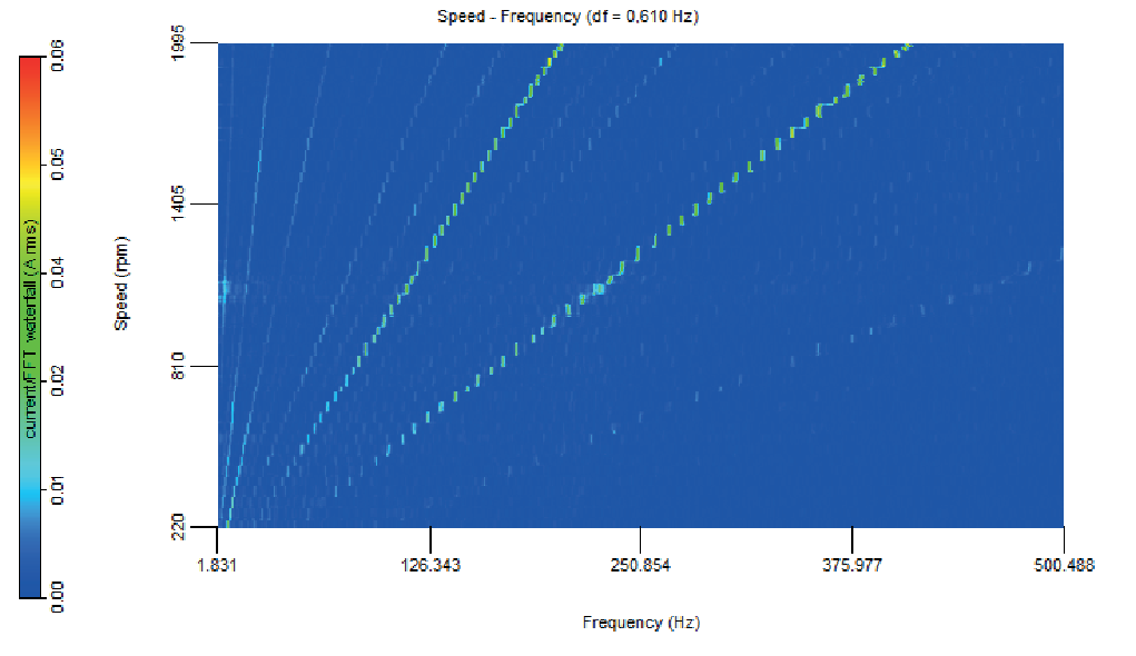
Initial measurements of the current revealed some unexpected behavior. The current signal showed a considerable amount of noise, and the reason was investigated. In particular, specific higher-order frequencies appeared when inspecting the FFT of the current signal. It was hypothesized that these higher-order frequencies, which are not captured by the linear or non-linear system model, could be caused by unmodeled system behavior. Examples could be, for instance, the gear-meshing frequency, shaft misalignment, unbalance in the shafting system, propeller blade passing frequencies, or cogging of the electric motor due to a discrete number of permanent magnets and the gaps in between them.
To obtain insight into the cause of the higher-order frequencies, an order tracking of current in the motor speed range from 220 to 1995 rpm was carried out, as shown in Figure 5 and Figure 6. The figures reveal that although many harmonic frequencies were present in the current signal, the 6th and 12th harmonics of motor speed were particularly dominant. A similarly strong 6th and 12th harmonic were found when carrying out the test with disconnected gearwheels. Manual rotation of the motor shaft revealed a strong cogging effect at 6 times the motor shaft rate. Based on this it is concluded that the root cause of the higher-order frequencies lies in the interaction between rotor and stator of the electric motor.
Filtering has been considered to reduce the visually disturbing effect of cogging-related harmonics from the plotted current signal. However, by filtering additional phase lag would be introduced, which would result in less steep current increase following a step in voltage, and it could reduce the amplitude of the current signal following a sinusoidal voltage input. In the end, it was decided to show the unfiltered current measurements.
In addition, the motor speed signal showed unexpected behavior, which appeared to be caused by the sensor. A sketch of the encoder disk used in the experiments is shown in Figure 7. It is a round disk with 15 holes, which causes 15 pulses per revolution, generated by a photosensitive sensor. The motor speed is derived from the time interval between two upcoming flanks of the pulses. The resulting motor speed signal as shown in Figure 8 shows a repeating sequence of 15 motor speed values, indicating that the angle between the holes varied slightly around 360/15 = 24°. No further corrections have been made to the signal, which explains the relatively ”noisy” motor speed signal presented in the following sections.
5. Results and Discussion
In this section, the results obtained with the different identification techniques are reported. Both the identification and validation analyses are carried out in both time and frequency domains.
In Table 4 the steady-state operating points recorded during the staircase experiment are reported. The time domain approach (1) uses all the five operating points to determine four out of the total of six unknown parameters. To determine the remaining two parameters and the transient response from operating point C to D is used.
The other identification approaches focus on operating point C. The reason to choose this point is that it corresponds to around 75% of the maximum supply voltage, which is a reasonable value thinking about the design of a full-scale propulsion plant.
First, the resulting parameter sets of the different approaches are reported in Table 5 to appreciate the difference in terms of numerical value. The parameters derived from the spectral approach (5) are not reported as will be explained later. The table shows that the parameters obtained with the methods were of the same order of magnitude, but differences up to ≈100% were present. The effect of the different sets of parameters on the simulated system behavior is shown in the validation graphs.
5.1. Results Time Domain Analysis (1)
The time domain identification method was used to derive the parameters from the staircase experiment. The supply voltage during this experiment is shown in Figure 9, while the measured motor speed and current are shown in Figure 10 and Figure 11.
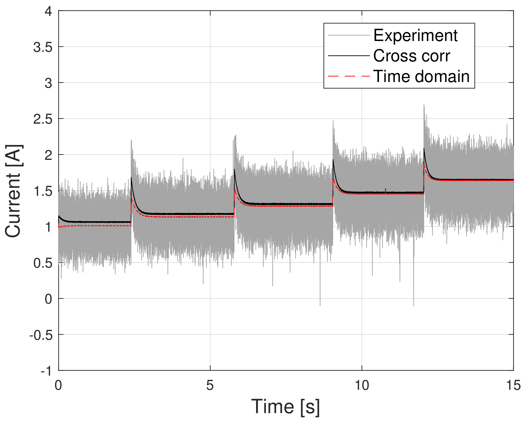
Following the procedure outlined earlier, the five steady-state operating points during the staircase experiment were determined, and the parameters , , , and were derived by the least-squares method. Subsequently, the transient response of motor speed and current, following the voltage step from C to D, was used to determine the parameters and .
The resulting set of parameters was implemented in the non-linear simulation model, and by using the staircase voltage signal as input, the model and its parameters are verified. The result is shown as the dashed red line in Figure 10 and Figure 11. The motor speed matched the experimental data well: the stationary value errors were within 3% at all voltage levels. Close inspection of the transient responses showed that these were also captured well. The simulated current signal had to be compared with very noisy experimental data, as explained earlier. Nevertheless, the static values seemed to be predicted well. Close inspection of the transient response shows that the simulation model could catch the timing and the initial steep slope of the current, but it was not able to represent the peak values in the current. It is concluded that this is either due to the limitations of the mathematical model, which might be too simple to describe the real physical phenomena, or due to the quality of the measured current signal.
Figure 10 and Figure 11 also show the results of the correlation approach, in continuous black line. However, since the staircase experiment was not used to determine the parameters using the correlation approach, this can be seen as validation of that method.
Figure 10 shows that the correlation approach predicted the motor speed behavior nearby the linearization point well, although the error between simulated and experimental data increased moving further away from the nominal operating point that was used in the sine experiments. Figure 11 shows that, compared to the time domain approach, the correlation approach was better able to predict the transient, although this method was also not able to catch the maximum current value.
To have an independent validation for the time-domain method, an experiment based on a mix of different input voltages, as shown in Figure 12, was used. Figure 13 shows that the parameter sets found by both methods led to similar dynamic behavior as the experiment, although a constant bias of around 50 rpm between simulated and sampled time histories was present. Figure 14 shows that the two parameter sets, in general, gave good correlation with the experiment, but both were unable to capture the maximum amplitudes of the current, which was particularly evident in the “sine wave” part from t = 10–13 s.
5.2. Results of Frequency Domain Analysis (4 and 5)
The single frequency testing method was applied in the nominal operating point C that is defined in Table 4. The results of the nine experiments are plotted as asterisks data points in the Bode plots shown in Figure 15 and Figure 16. The data points at 1000 and 5000 rad/s were discarded, as closer inspection of the time signals showed that the signal-to-noise ratio was too low to lead to meaningful results.
Based on the data points, the procedure as outlined above was followed, leading to the estimated parameters as listed in Table 5. The following values were iteratively determined from the experimental data points: rad/s, rad/s, rad/s, , . Note that the locations of the poles and zero were read from the dB versions of the Bode plots.
To verify whether the estimation procedure was followed correctly, the found parameters were implemented in the transfer functions (12) and (13), which are plotted as solid lines in Figure 15 and Figure 16. The agreement in trend and absolute numbers indicates that the procedure was followed correctly and that the linearized model can capture the reality well in the operating point under consideration. Validation in the time domain of the parameter set obtained with this method is reported in the previous section.
The shape of the transfer function for motor speed shows that up to 2 rad/s the response remained flat but then quickly dropped off due to the inertia of the drive train. The transfer function for current showed a flat response up to 1 rad/s and then started to rise due to the zero in the transfer function. Around 20 rad/s, it flattened out due to the inertia of the drive train. Somewhere after 1000 rad/s it dropped off, due to the electric pole, indicating that the current cannot follow the voltage variations anymore.
Figure 15 also shows the transfer function based on the parameter set derived with the time-domain approach. The response to low frequencies was good, but the drop in gain started slightly too early, which aligns with the low estimate of in Table 5. In Figure 16 a substantial deviation from the data points is visible at frequencies higher than 10 rad/s, although the shape is clearly recognizable.
Finally, Figure 15 and Figure 16 also show the results from approach 5. Between 0.4 and 400 rad/s the method resulted in a non-parametric frequency response that aligned well with the asterisk data points. In hindsight, the duration of the experiment should have been extended up to 1–2 min or even longer, instead of 30 s. A more extended trial would allow the estimation of the transfer function up to lower frequencies and would allow for further averaging over multiple data blocks to smooth out irregularities in the results. At frequencies above 400 rad/s, the signal-to-noise ratio dropped leading to bumps in the estimated frequency response.
Although the parameter estimation based on noise injection could be used to assess the unknown parameters from the frequency response, this is not performed here but is left for a further study on the potential of spectral methods for ship drive train identification.
6. Future Outlook
Application of the identification procedures on-board a real ship is expected to make the analytic derivations more complex because the system will, in that case, include other/additional components such as, for instance, a diesel engine and engine speed governor. This introduces at least one extra state equation due to the integral term in the PI(D) governor. An additional state, due the longitudinal equation of motion, and additional parameters would be added if the approach would be extended to free sailing instead of bollard pull conditions. The effect of such additions on the ability to determine parameters needs to be investigated in the future. On the positive side, it has to be noted that in reality it is not likely that all ship drive-train parameters are unknown, which helps to determine estimates of other unknown or more uncertain parameters. More work is required to investigate what parameter estimation procedure would be required for a real ship and drive train.
In the authors’ opinion, in the future the presented algorithms could potentially be part of a condition-based maintenance system. By monitoring parameter variations of a propulsion drive train in real time, it could be possible to detect the degradation (or malfunction) of the machinery, and perhaps even to identify the root cause. For instance, an increase in friction coefficient could mean wear in the bearings, an increase in could mean that the propeller needs to be cleaned, etc. Another possible use of the presented techniques is to assess the correspondence between the design values with the real one, in fact, during the shipbuilding progress some change, or unexpected modification, can modify the original design values.
7. Conclusions and Recommendations
In this paper different parameter identification techniques were discussed and applied to experimentally determine the unknown parameters of a model scale ship drive train in bollard pull conditions.
A set of dedicated experiments was conducted using different DC voltage signals. In all tests the current was affected by a strong noise due to motor cogging. It is therefore recommended to use an electric motor with less strong cogging effect for future experiments. Moreover, the 15 holes encoder was found to give a low-quality motor speed measurement and should be improved.
Three different approaches to determine the unknown DC-electric propulsion plant parameters are discussed including their merits and weaknesses. For now, all three approaches remain candidates to be part of a (real-time) full-scale parameter identification system, which is one of the primary goals.
Two obtained parameter sets have been implemented in a simulation model, and the results were validated against independent measurements, both in the frequency and in the time domains. The time domain results obtained by implementing both parameter sets in the model compared well against the measurements, although differences were present.
In order to move towards firm conclusions about the value of the applied parameter estimation methods for condition monitoring, it is recommended to consider the sensitivity and uncertainty related to the approaches. This recommendation is supported by the relatively large differences between the parameter sets as determined in this paper, and the relatively small differences in time domain response.
Author Contributions
Conceptualization, A.V. and M.M.; methodology, A.V. and M.M.; software, A.V. and M.M.; writing—original draft preparation, A.V. and M.M.; writing—review and editing, A.V. and M.M.; experimental testing A.V. and M.M. All authors have read and agreed to the published version of the manuscript.
Funding
This research was partly supported by Maritime by Holland (in Dutch: NML) and the Ministry of Economic Affairs of the Netherlands. Furthermore, this research was partly funded by University of Genoa within the program “Incentive for research periods abroad”.
Acknowledgments
The authors want to acknowledge Eng. Vittorio Garofano of Delft University of Technology for his essential support during the experimental campaign.
Conflicts of Interest
The authors declare no conflict of interest.
Nomenclature
| Boa | ship breadth | [m] |
| C | constant | |
| c | constant | |
| D | propeller diameter | [m] |
| e | general exponent | |
| FBP | bollar pull force | [N] |
| Ip | moment of inertia | [kgm2] |
| ia | motor current | [A] |
| igb | gearbox ratio | [-] |
| J | advance ratio | [-] |
| K | constant | |
| KQ | torque coefficent | [-] |
| KT | thrust coefficent | [-] |
| Ke | motor speed constant | [V/rad/s] |
| Ke | motor back EMF constant | [Nm/A] |
| kp | propeller number | [-] |
| Loa | ship length | [m] |
| La | motor inductance | [H] |
| Mb,em | motor torque | [Nm] |
| Mf | friction torque | [Nm] |
| Mp | delivered torque | [Nm] |
| Q | open water torque | [Nm] |
| Ra | motor resistance | [Ω] |
| s1 | first pole | [-] |
| s2 | second pole | [-] |
| T | propeller thrust | [N] |
| t | time | [s] |
| t | thrust deduction factor | [-] |
| Ua | voltage supply | [V] |
| Δ | ship displacement | [kg] |
| ζ | ratio of time constants | [-] |
| ηR | relative rotative efficiency | [-] |
| ηtrm | shaftline efficiency | [-] |
| ρ | water density | [kg/m3] |
| τem | electric time constant | [s] |
| τω | mechanical time constant | [s] |
| τω,e | effective mechanical time constant | [s] |
| ωem | motor speed | [rad/s] |
| ωp | propeller speed | [rad/s] |
| ω | frequency | [rad/s] |
| Subscripts and Superscripts | ||
| 0 | nominal | |
| * | normalized | |
| small increment | ||
Appendix A. Normalisation and Linearisation
Assume a variable that is the product of powers of other variables:
where c is a constant multiplier and e is a constant exponent. In an equilibrium point the variable Z equals
If, by definition,
then
Now that the constant value c has been removed by the normalization, the next step is to remove the non-linearity from Equation (A5). Differentiation of Equation (A3) by using the chain rule gives
Near equilibrium , and become small increments , and . Division of by delivers and likewise . Substitution of this in Equation (A6) gives
Taylor series expansion of Equation (A7) and neglecting the second and higher order terms leaves
which by introduction of the shorthand notation for differential increment:
this can be written as
The latter equation relates the relative change in output Z to the relative change in inputs X and Y, where the constant e, which was present as an exponent in the original Equation (A2), has changed to a constant multiplication factor. Secondly the multiplication of X and Y has turned into a summation. For further background on the linearization process, reference is made to Dorf and Bishop [33] and Franklin et al. [34].
The demonstrated concepts of normalization and linearization are the basis for the following section where they will be applied in the linearization of the system model.
Appendix B. Derivation of Linearized System Model
The electrical circuit of the DC motor is modeled by
All three right hand side terms vary around equilibrium:
In static conditions the right hand side of Equation (A11) equals zero:
This means that only the small increments are of importance:
Division of all terms of Equation (A13) by nominal supply voltage minus the nominal emf or alternatively by its equivalent gives
This can be shortened to
in which the subscript is intentionally dropped from because and where
The shaft dynamics including constant friction term are described by
in which shaft inertia is assumed constant implying that change of mass of water, entrained by the propeller, is neglected. The brake motor torque is related to current by
In steady nominal condition the driving torque and the load-torque are equal:
Subtracting Equation (A20) from Equation (A19) shows that only the small increments are of importance:
Normalizing all terms with nominal motor torque gives
in which the subscript is intentionally dropped. The integration constant is defined as
After noting that the multiplier in the second term of the right hand side of Equation (A21) can be written as
and implementing
the normalised linearised differential equation for shaft rotation is given by
Introduction of the Laplace operator into Equation (A24) and re-arranging gives
which can be shortened by introduction of the effective time-constant:
such that
Similarly, introduction of the Laplace operator in the differential equation for current Equation (A15) and reordering gives
Substitution of Equation (A28) into Equation (A27) and reordering gives the transfer function from supply voltage to rotation speed:
In a similar way substitution of Equation (A27) into Equation (A28) and reordering gives the transfer function from supply voltage to current:
If we define
and
then the characteristic equation can be written as
The two exact roots of Equation (A31) can now be determined by the ABC formula:
which can be written as
The electrical time constant is much smaller than the effective time constant for the shaft; therefore, . Application of Taylor expansion for the square root operation and leaving out second order terms gives
Another Taylor expansion for the inverse square operation gives
Further simplification gives the two approximate poles as
and
Besides the two system poles, transfer function (A30) has a single zero which lies at
The DC-gain of transfer function (A29) is given by
The DC-gain of transfer function (A30) is given by
Appendix C. Step Response of Motor Speed and Current
The exact response of motor speed to a unit step in voltage is given by
in which . However, because , the step-response can be approximated by a first order system response:
The derivation of the step response of current starts with Equation (A30), which can be written as the summation of an overdamped second order lowpass (LP) system and a second order bandpass (BP) system:
The step response of the lowpass system is given by
with . Again, because , this can be approximated by a first order system response:
References
- Martelli, M.; Figari, M. Real-Time model-based design for CODLAG propulsion control strategies. Ocean Eng. 2017, 141, 265–276. [Google Scholar] [CrossRef]
- Vrijdag, A.; Stapersma, D.; van Terwisga, T. Control of propeller cavitation in operational conditions. J. Mar. Eng. Technol. 2010, 9, 15–26. [Google Scholar] [CrossRef] [Green Version]
- Cipollini, F.; Oneto, L.; Coraddu, A.; Murphy, A.J.; Anguita, D. Condition-Based Maintenance of Naval Propulsion Systems with supervised Data Analysis. Ocean Eng. 2018, 149, 268–278. [Google Scholar] [CrossRef] [Green Version]
- Mizythras, P.; Boulougouris, E.; Theotokatos, G. Numerical study of propulsion system performance during ship acceleration. Ocean Eng. 2018, 149, 383–396. [Google Scholar] [CrossRef] [Green Version]
- Martelli, M. Marine Propulsion Simulation; De Gruyter Open: Berlin, Germany, 2015. [Google Scholar]
- Geertsma, R.; Negenborn, R.; Visser, K.; Loonstijn, M.; Hopman, J. Pitch control for ships with diesel mechanical and hybrid propulsion: Modelling, validation and performance quantification. Appl. Energy 2017, 206, 1609–1631. [Google Scholar] [CrossRef]
- Vrijdag, A.; Stapersma, D.; van Terwisga, T. Systematic modelling, verification, calibration and validation of a ship propulsion simulation model. J. Mar. Eng. Technol. 2009, 8, 3–20. [Google Scholar] [CrossRef]
- Ljung, L. System Identification: Theory for the User, 2nd ed.; Prentice Hall: Upper Saddle River, NJ, USA, 1999. [Google Scholar]
- Weerasooriya, S.; El-Sharkawi, M.A. Identification and control of a DC motor using back-propagation neural networks. IEEE Trans. Energy Convers. 1991, 6, 663–669. [Google Scholar] [CrossRef]
- Liu, X.Q.; Zhang, H.Y.; Liu, J.; Yang, J. Fault detection and diagnosis of permanent-magnet DC motor based on parameter estimation and neural network. IEEE Trans. Ind. Electron. 2000, 47, 1021–1030. [Google Scholar] [CrossRef]
- Lu, W.; Keyhani, A.; Fardoun, A. Neural network-based modeling and parameter identification of switched reluctance motors. IEEE Trans. Energy Convers. 2003, 18, 284–290. [Google Scholar] [CrossRef]
- Cirrincione, M.; Pucci, M.; Cirrincione, G.; Capolino, G. A new experimental application of least-squares techniques for the estimation of the induction motor parameters. IEEE Trans. Ind. Appl. 2003, 39, 1247–1256. [Google Scholar] [CrossRef]
- Wang, K.; Chiasson, J.; Bodson, M.; Tolbert, L.M. A nonlinear least-squares approach for identification of the induction motor parameters. IEEE Trans. Autom. Control 2005, 50, 1622–1628. [Google Scholar] [CrossRef]
- Yoerger, D.R.; Cooke, J.G.; Slotine, J.J.E. The influence of thruster dynamics on underwater vehicle behavior and their incorporation into control system design. IEEE J. Ocean. Eng. 1990, 15, 167–178. [Google Scholar] [CrossRef] [Green Version]
- Healey, A.J.; Rock, S.M.; Cody, S.; Miles, D.; Brown, J.P. Toward an improved understanding of thruster dynamics for underwater vehicles. IEEE J. Ocean. Eng. 1995, 20, 354–361. [Google Scholar] [CrossRef]
- Whitcomb, L.L.; Yoerger, D.R. Comparative experiments in the dynamics and model-based control of marine thrusters. In Proceedings of the OCEANS ’95 MTS/IEEE ’Challenges of Our Changing Global Environment’, San Diego, CA, USA, 9–12 October 1995; Volume 2, pp. 1019–1028. [Google Scholar] [CrossRef]
- Whitcomb, L.L.; Yoerger, D.R. Preliminary experiments in the model-based dynamic control of marine thrusters. In Proceedings of the IEEE International Conference Robotics and Automation, Minneapolis, MN, USA, 22–28 April 1996; Volume 3, pp. 2166–2173. [Google Scholar] [CrossRef] [Green Version]
- Whitcomb, L.L.; Yoerger, D.R. Preliminary experiments in model-based thruster control for underwater vehicle positioning. IEEE J. Ocean. Eng. 1999, 24, 495–506. [Google Scholar] [CrossRef] [Green Version]
- Bachmayer, R.; Whitcomb, L. Unsteady dynamics and control of marine thrusters. J. Acoust. Soc. Am. 1999, 105, 1300. [Google Scholar] [CrossRef]
- Bachmayer, R.; Whitcomb, L.; Grosenbaugh, M. An accurate four-quadrant nonlinear dynamical model for marine thrusters: Theory and experimental validation. IEEE J. Ocean. Eng. 2000, 25, 146–159. [Google Scholar] [CrossRef]
- Blanke, M.; Lindegaard, K.P.; Fossen, T.I. Dynamic Model for Thrust Generation of Marine Propellers. IFAC Proc. Vol. 2000, 33, 353–358. [Google Scholar] [CrossRef] [Green Version]
- Fossen, T.I.; Blanke, M. Nonlinear output feedback control of underwater vehicle propellers using feedback form estimated axial flow velocity. IEEE J. Ocean. Eng. 2000, 25, 241–255. [Google Scholar] [CrossRef]
- Smogeli, Ø.N. Control of Marine Propellers from Normal to Extreme Conditions. Ph.D. Thesis, Norwegian University of Science and Technology, Trondheim, Norway, 2006. [Google Scholar]
- Pivano, L.; Fossen, T.I.; Johansen, T.A. Nonlinear model identification of a marine propeller over four-quadrant operations. IFAC Proc. Vol. 2006, 39, 315–320. [Google Scholar] [CrossRef]
- Pivano, L.; Fossen, T.I.; Smogeli, Y.N.; Johansen, T.A. Experimental Validation of a Marine Propeller Thrust Estimation Scheme. Model. Identif. Control 2007, 28, 105–112. [Google Scholar] [CrossRef] [Green Version]
- Coraddu, A.; Oneto, L.; Ghio, A.; Savio, S.; Anguita, D.; Figari, M. Machine learning approaches for improving condition-based maintenance of naval propulsion plants. Proc. Inst. Mech. Eng. Part M J. Eng. Marit. Environ. 2016, 230, 136–153. [Google Scholar] [CrossRef]
- Altosole, M.; Campora, U.; Martelli, M.; Figari, M. Performance Decay Analysis of a Marine Gas Turbine Propulsion System. J. Ship Res. 2014, 58, 117–129. [Google Scholar] [CrossRef]
- Carlton, J.S. Marine Propellers and Propulsion; Buttersworth-Heineman Ltd.: Oxford, UK, 2007. [Google Scholar]
- Stapersma, D.; Vrijdag, A. Linearisation of a ship propulsion system model. Ocean Eng. 2017, 142, 441–457. [Google Scholar] [CrossRef]
- Vrijdag, A.; Stapersma, D. Extension and application of a linearised ship propulsion system model. Ocean Eng. 2017, 143, 50–65. [Google Scholar] [CrossRef]
- Welch, P. The use of fast Fourier transform for the estimation of power spectra: A method based on time averaging over short, modified periodograms. IEEE Trans. Audio Electroacoust. 1967, 15, 70–73. [Google Scholar] [CrossRef] [Green Version]
- Balmer, L. Signals and Systems: An Introduction, 2nd ed.; Prentice Hall: Upper Saddle River, NJ, USA, 1997. [Google Scholar]
- Dorf, R.C.; Bishop, R.H. Modern Control Systems, 9th ed.; Prentice Hall: Upper Saddle River, NJ, USA, 2001. [Google Scholar]
- Franklin, G.F.; Powell, J.D.; Emami-Naeini, A. Feedback Control of Dynamic Systems; Addison-Wesley: Reading, MA, USA, 1986; Volume 5. [Google Scholar]
Figure 1.
Tito Neri overview.

Figure 2.
Tito Neri azimuthing thrusters from astern.

Figure 3.
Schematic representation of Tito Neri drive train.

Figure 4.
Block diagram of experimental setup.

Figure 5.
Order waterfall plot.

Figure 6.
FFT waterfall plot.

Figure 7.
Encoder disk.

Figure 8.
Magnification of motor speed time history.

Figure 9.
Voltage time history of the staircase test.

Figure 10.
Motor speed time history of the staircase test.

Figure 11.
Current time history of the staircase test.

Figure 12.
Voltage time history.

Figure 13.
Motor speed time history.

Figure 14.
Current time history.

Figure 15.
Bode plot of .

Figure 16.
Bode plot of .


Table 1.
Main particulars of Tito Neri.
| 0.97 | [m] | |
| 0.32 | [m] | |
| draft forward/aft | 0.10/0.13 | [m] |
| displacement with/without battery | 15.4/13.5 | [kg] |
| upper bevel gear teeth ratio | 13:39 | [-] |
| total gear reduction ratio | 3 | [-] |
| Propeller diameter D | 0.065 | [m] |
Table 2.
Experimental FRD based on single sinusoidal testing, followed by processing with the correlation approach.
Table 2.
Experimental FRD based on single sinusoidal testing, followed by processing with the correlation approach.
| [rad/s] | 0.3 | 1 | 5 | 10 | 20 | 100 | 500 | 1000 | 5000 |
|---|---|---|---|---|---|---|---|---|---|
| [-] | 0.71 | 0.79 | 1.62 | 2.31 | 2.94 | 3.08 | 2.99 | 2.90 | 2.11 |
| [deg] | 8.6 | 19.4 | 37.7 | 31.3 | 19.6 | 3.5 | −4.5 | −8.8 | −26.8 |
| [-] | 1.24 | 1.18 | 1.05 | 0.81 | 0.54 | 0.12 | 0.02 | 0.01 | 0.00 |
| [deg] | −2.2 | −7.0 | −26.2 | −45.4 | −64.3 | −95.5 | −144.9 | 146.3 | 20.7 |
Table 3.
Experimental test matrix.
| Test | Identification | Validation |
|---|---|---|
| Staircase | yes (1) | yes (4) |
| 9 × Sinusoidal | yes (4) | yes (1,4,5) |
| White noise | yes (5) | |
| Mix of signals | yes (1,4) |
Table 4.
Evaluated operating points.
| Operating Points | ||||||
|---|---|---|---|---|---|---|
| A | B | C | D | E | Unit | |
| 3.91 | 4.91 | 5.89 | 6.88 | 7.87 | [V] | |
| 117 | 163 | 215 | 255 | 295 | [rad/s] | |
| 1.00 | 1.13 | 1.29 | 1.44 | 1.62 | [A] | |
Table 5.
Identified parameters.
| METHOD | I | IV | Unit |
|---|---|---|---|
| 4.87 × 10 | 6.03 × 10 | [H] | |
| 1.37 × 10 | 1.83 × 10 | [Nm/A] | |
| 2.31 | 1.51 | [] | |
| 1.72 × 10 | 3.18 × 10 | [kg m] | |
| 1.23 × 10 | 1.70 × 10 | [Nm] | |
| 1.02 × 10 | 1.36 × 10 | [-] |
Publisher’s Note: MDPI stays neutral with regard to jurisdictional claims in published maps and institutional affiliations. |
© 2021 by the authors. Licensee MDPI, Basel, Switzerland. This article is an open access article distributed under the terms and conditions of the Creative Commons Attribution (CC BY) license (http://creativecommons.org/licenses/by/4.0/).
Share and Cite
MDPI and ACS Style
Vrijdag, A.; Martelli, M. Parameter Identification of a Model Scale Ship Drive Train. J. Mar. Sci. Eng. 2021, 9, 268. https://0-doi-org.brum.beds.ac.uk/10.3390/jmse9030268
AMA Style
Vrijdag A, Martelli M. Parameter Identification of a Model Scale Ship Drive Train. Journal of Marine Science and Engineering. 2021; 9(3):268. https://0-doi-org.brum.beds.ac.uk/10.3390/jmse9030268
Chicago/Turabian StyleVrijdag, Arthur, and Michele Martelli. 2021. "Parameter Identification of a Model Scale Ship Drive Train" Journal of Marine Science and Engineering 9, no. 3: 268. https://0-doi-org.brum.beds.ac.uk/10.3390/jmse9030268
Note that from the first issue of 2016, this journal uses article numbers instead of page numbers. See further details here.