Article

Spatial Analysis of the Fishing Behaviour of Tuna Purse Seiners in the Western and Central Pacific Based on Vessel Trajectory Data

1
College of Science, University of Shanghai for Science and Technology, Shanghai 200093, China
2
Key and Open Laboratory of Remote Sensing Information Technology in Fishing Resource, East China Sea Fisheries Research Institute, Chinese Academy of Fishery Sciences, Shanghai 200090, China
3
Key Laboratory of East China Sea & Oceanic Fishery Resources Exploitation and Utilization, Ministry of Agriculture, Shanghai 200090, China
4
College of information, Shanghai Ocean University, Shanghai 201306, China
*
Author to whom correspondence should be addressed.
The author contributed to the work equally and should be regarded as co-first authors.
J. Mar. Sci. Eng. 2021, 9(3), 322; https://0-doi-org.brum.beds.ac.uk/10.3390/jmse9030322
Submission received: 21 January 2021 / Revised: 10 March 2021 / Accepted: 11 March 2021 / Published: 15 March 2021
(This article belongs to the Section Marine Biology)

Abstract

:
The Western and Central Pacific Oceans are the primary operational areas of tuna purse seiners worldwide. Describing and analysing the fishing behaviour of vessels is highly significant for the protection of sustainable tuna resources. This study uses Automatic Identification System (AIS) data of 130 tuna purse seiners from July 2017 to May 2018 and uses data mining methods to identify the operating status of tuna purse seiners; describes the spatial characteristics of fishing intensity and the distribution of hot spots; and analyses vessel spatial characteristics to describe their fishing behaviour. The results show that the tuna purse seiner speed has a marked bimodal distribution, which corresponds to high-speed transiting and low-speed seine operation. Additionally, from July to September 2017, the amount of fishing effort invested by tuna purse seiners was lower than that in other months. The tuna purse seiner activity range includes 120° E–60° W, 30° S–30° N, and the activities for fish and seine operations are primarily concentrated at 140° E–150° W, 15° S–15° N. There are differences between the space for fishing search operations and space where fishing events took place in each month. Spatial analysis shows that the high-speed transiting fishing effort map covers a large area, while seine fishing covers a small area. The global spatial autocorrelation analysis shows that the fishing effort devoted to searching for fish stocks has a spatial distribution pattern of aggregation and close aggregation. The results of a hot-spot analysis show that the hot spots on a heat map for finding fish, which are closely spatially clustered, correspond to vessels searching for fish concentration areas and seine operation areas. Correlation testing shows that under a 5° × 5° grid, there is a high positive correlation between the fishing effort invested in finding fish stocks and the yield data, nets (r > 0.8), and a moderate correlation with catch per unit of effort(CPUE) (r > 0.3). Based on vessel behaviour, the location of the fish school can be directly determined, and the distribution of fish clusters and fishing grounds can be predicted. This study can aid in managing tuna purse seiners in the Western and Central Pacific Oceans and analysing changes in fishery resources.

1. Introduction

Tuna is an economically important species in pelagic fisheries. More than 50% of the world’s primary tuna production comes from the Western and Central Pacific [1]. The status of tuna resources has decreased from the historical high level, and tuna has become a hot spot of national and regional concern; thus, it is important to assess tuna resources for sustainable development and management. Resource assessment is an important part of fishery resource management; however, traditional resource assessment cannot quantify the fishing intensity of tuna fishery resources and living waters; thus, the management and monitoring of vessels are equally important. Due to the large area spanned by the oceans, it is not feasible for traditional vessels to perform full public supervision. Recent studies have shown that space behaviour can show hot spots of fishing activities and their relationship with external factors, and there have been certain relevant studies in offshore trawling fisheries [2,3].
In a pelagic tuna fishery, Nicolas Bez et al. [4] used vessel monitoring system (VMS) data to study and quantify the spatial dynamics of tuna purse seine fishing activities in the Seychelles in the Indian Ocean. With the high coverage rate of VMS data and many applications in offshore fisheries, its positioning accuracy and near real-time performance have been widely used in fishing effort estimation and fishery resource assessment. However, the temporal resolution of VMSs is relatively low, and the method used to analyse VMS data may affect the estimation of fishing intensity [5], particularly the size of the grid cell used for analysis, which affects fishing intensity estimates [6]. Additionally, VMS data are a closed system that is typically difficult to obtain publicly [7].
Automatic identification system (AIS) data have a high time resolution and provide rich information, such as the distribution of vessels, vessel dynamics and vessel trajectories, which can be publicly obtained [8]. AIS data can be used to reshape the navigation trajectory of vessels through a series of discrete point data, which has been successfully used in maritime supervision, collision avoidance of vessels, target tracking and auxiliary decision-making. Vessel trajectory data were used to identify the status of the vessels, describe fishing effort and analyse the fishing space of vessels and other aspects of fishery application research. Yang Shenglong et al. [9] used AIS information to build a support vector machine (SVM) model by mining the operating speed and heading characteristics of longline vessels to establish a fishing ground operation status recognition model and determine the fishing intensity information of the fishing ground. Yuan Zuohui et al. [10] used the Moran index in global spatial autocorrelation and the hot-spot analysis method in local spatial autocorrelation to show that the fishing effort of tuna longline vessels in the central and western Pacific is spatially autocorrelated and has a significant aggregation and distribution pattern. Kroodsma [11] used a convolutional neural network to identify the operational status of tuna purse seine fishing and discovered that the hot spots of fishing activities on a global scale are related to fishing methods, marine environment and culture, but without seasonal analysis. Cimino [12] studied the temporal and spatial fishing trends of vessels by considering marine environmental factors and used the boosting regression tree (BRT) model to analyse the internal relationship between fishing behaviour and environmental factors to identify fishing vessels and their dependence on the environment.
There are many analyses of the fishing effort of tuna longline vessels. Tuna purse seine fishing is the primary type of tuna production [1,13]. Currently, there is still little information about spatial analysis of the fishing behaviour of regional tuna purse seiners. In this paper, AIS data were used to conduct spatial analysis of the fishing activities of tuna purse seiners in the Western and Central Pacific, and the temporal and spatial variations in fishing efforts and fishing intensity of these vessels were clarified to provide support for fishery resource management.

2. Data Pre-Processing

2.1. Data Source and Data Pre-Processing

In this study, data on 191 Pacific tuna purse seiner vessels were collected from the literature [11], Global Fishing Watch Data and the Western and Central Pacific Fisheries Commission (WCPFC) based on Maritime Mobile Service Identify (MMSI) and ship name. Based on the MMSI number, AIS dynamic time-series data such as date, longitude and latitude, course and speed were extracted. The time range of AIS data in this study covers a total of 11 months from July 2017 to May 2018. Of the 191 vessels, 43 MMSI had no AIS data. A total of 148 MMSI vessels had AIS data, 59 MMSI vessels had AIS data for all months and the other 89 had only AIS data for the months September, November and December 2017 and from January to May 2018.
The AIS data of these 148 fishing vessels were selected based on the MMSI number and sorted by date and time, and data with repeated times were eliminated. Based on personal interviews with fishermen, experience of our former fisheries observers and our statistical results, the speed of the tuna purse seine is generally below 15 knots. The selected speed was 0–15 knots of AIS data, and the data of speeds greater than 15 knots were eliminated. The date was converted into “year”, “month”, “day”, “hour”, “minute”, “second”, and select “longitude”, “latitude”, “course”, and “speed”. The time difference between two vessel positions before and after each vessel was calculated using the following formula:
T i , j = T i , j T i 1 , j
where T i , j and T i 1 , j are the time of the two consecutive vessel positions in the trajectory of vessel j ; the difference between the two is the time interval T ; and the unit is hour.
From the time interval of more than 24 h of data points, excluding data points with a time interval greater than 24 h, we finally obtain a total of 8,117,450 data points for these 148 tuna purse seiners from July 2017 to May 2018.
The study obtained the production data of tuna purse seiners from the Western and Central Pacific Fishery Commission (WCPFC). The data included longitude, latitude, catches, and net times. The time resolution is one month, and the spatial resolution is 5° × 5°. The formula for calculating the catch per net time is as follows [14]:
C P U E = C i n i
where C i is the catch of vessels in the ith grid in the study area, n i refers to the total number of nets used by vessels for fishing operations in the corresponding ith grid, i is the number of grids, and C P U E is the catch per unit effort in tons.

2.2. Study Area

Based on the AIS information of 148 tuna purse seiners, the AIS data of the vessels in the Pacific through the spatial track points involved a total of 130 vessels. The spatial trajectory distribution of the 130 vessels over 11 months is shown in Figure 1. Based on Figure 1, 120° E–60° W and 30° S–30° N were selected as the study areas in this paper.
A total of 130 tuna purse seiner vessels were classified based on the MMSI. A total of 130 tuna purse seiners belong to 14 countries and regions. Among all vessels, the United States has the most vessels (27), followed by South Korea (22), Papua New Guinea (17), Philippines (15), The Federated States of Micronesia (13), Kiribati (9) and so on. China has 8 vessels, and the country and region with the least number has only one vessel.

3. Methods

3.1. Fishing Behaviour of Tuna Purse Seiners

Seiners are vessels that primarily catch the fast-moving upper strata of the ocean, and a seine is a long net suspended vertically by a vessel or separate small boat on the sea or around a shoal of fish. To chase and round up fish, the purse seine is typically dragged at a certain speed. When information is received about the presence of dense schools of fish in an area, the vessels move quickly to the central zone of the fishery. Tuna swim faster, and seine nets must be set quickly to avoid fish escaping. Therefore, when fishing schools of tuna, the purse seine is moved at high-speed. Once the net is completely around the fish, the bottom of the net is pulled open, and the net is dragged away. A seine operation is defined as the time between the time the net surrounds the fish and the end of the fishing operation when the net is lifted out of the water, and the length of the operation may vary from an hour to several hours depending on the catch. During this period, seiners remain more or less stationary, typically at a slow speed of approximately 2.5 knots or less on the surface of the sea [15,16]. Second, in addition to specific operating speed characteristics, tuna purse seiners must adhere to specific time characteristics; thus, tuna purse seiners typically search for fish stocks and fishing operations only during the day and rest at night.

3.2. Different Trajectory Point Mining Method

Vessels set their nets quickly, but fishing may last several hours, during which time the speed of the vessel remains low. Based on these characteristics of tuna purse seine operation and the literature [16], this paper uses day/night and speed thresholds to identify the operating status of tuna purse seiners. The calcSol function in the solaR package was used to calculate the brightness of each locus point [17], and the daytime locus point was extracted with a brightness value greater than zero. In this paper, based on speed statistics and the literature [4], the threshold speed V1 and the brightness value are greater than zero to extract the operating trajectory points of the tuna purse seiners during net fishing, and the threshold speed V2 and the brightness value are greater than zero to extract high-speed transiting track points. The track points discriminant formula is as follows:
P f i s h i n g = { 1                             v V 1       a n d       c 0 0                                               e l s e
P s e a r c h i n g = { 1                             v V 2       a n d       c 0 0                                                     e l s e
where V 1 and V 2 are the speed ranges under the conditions of net fishing at low speed and high-speed transiting behaviour, respectively; and c is the brightness value, where c = 0 at night. When P f i s h i n g = 1 , we assume that a vessel is working (i.e., collecting the net for fish); when P s e a r c h i n g = 1 , we assume that a vessel is transiting or looking for or chasing schools of fish.

3.3. Definition of Fishing Intensity and Fishing Effort

Fishing effort is a measure of the human effort involved in fishing activities. In this paper, the time spent by tuna purse seiners on the sea to catch tuna, including search and chasing schools of fish and net fishing, is defined as the amount of fishing effort. The fishing intensity measures the time spent by all tuna seiners in each grid unit within a given time range.
To separately analyse the temporal and spatial distribution of vessel input under the two types of behaviours of high-speed transiting and harvesting nets, we identify the data of each trajectory point, count the fishing boats in different states, and calculate the fishing effort between two points in the corresponding sailing trajectory. The formula is as follows:
F E i , j = T i , j × P f i s h i n g
S E i , j = T i , j × P s e a r c h i n g
where P f i s h i n g and P s e a r c h i n g are the operating status of vessel j at position i ; F E i j is the fishing effort invested by the vessel under the net fishing behaviour; and S E i j is the fishing effort invested by the vessel in the act of high-speed transiting.
Within a certain period of time, the fishing intensity of the k operating grid in the fishery area is defined as the sum of the fishing efforts of all vessel position points within the grid in hours, and the calculation formula is as follows:
E k = j = 1 N i = 1 M E i , j
where N is the total number of vessels in the grid, and M is all position points of vessel j in the grid. E i , j is the fishing effort invested by fishing vessel j at the i 1 to i spatial positions in the trajectory of the voyage in hours, including F E i , j and S E i , j .

3.4. Spatial Analysis Method

3.4.1. Global Moran Index Parameter Calculation

To understand the global spatial distribution pattern of the fishing effort of tuna purse seiners studied in the study area, the global Moran’s index from the spatial autocorrelation analysis was used for measurement, and its formula is as follows [18]:
I = n i = 1 n j = 1 n w i , j z i z j ( i = 1 n j = 1 n w i , j ) i = 1 n z j 2 ,           ( i j )
where n represents the number of samples; z i and z j are the deviations of the attributes of elements i and j from the mean values of all sample attributes; and w i , j is the spatial weight between element i and element j . If element i and element j are adjacent, then w i , j = 1 ; otherwise, w i , j = 0 .
The range of the global Moran index is −1~1. If the value is greater than 0, the elements are clustered throughout the study area. The closer the value is to 1, the higher the degree of aggregation the distribution is. If the value is below 0, the elements are discretized throughout the study area. The closer the value is to −1, the higher the degree of discrete the distribution is. If the value is equal to 0, the elements are randomly distributed. In the ArcGIS software environment, the Global Moran’s I tool returns the Z score and p value, where the Z score is a multiple of the standard deviation, and a larger Z indicates that the elements are clustered and distributed. The p value refers to the probability that the geographical space elements are randomly distributed throughout the space, and a small p value indicates that the spatial distribution mode is less likely to be randomly distributed.

3.4.2. Calculation of Hot-Spot Analysis Parameters

To understand the local spatial distribution pattern of fishing effort of tuna purse seiners in the study area, the pattern was measured using hot spot analysis statistics and the spatial autocorrelation analysis method. Hot spot analysis can identify high and low-frequency locations of fishing efforts with statistical significance. Its formula is as follows [19]:
G i * = j = 1 n w i , j z j X ¯ j = 1 n w i , j S n j = 1 n w i , j 2 ( j = 1 n w i . j ) 2 n 1
where n , z i , z j and w i , j represent the meanings of Formula (8); X ¯ is the mean value of all the sample attributes; and S is the standard deviation.
In the ArcGIS software environment, the hot-spot analysis tool returns Z scores and p values, which are similar to the Z scores and p values returned by Global Moran’s I. A statistically significant positive Z score indicates hot spots, and the higher the Z score, the closer the hot spots are clustered. Negative values represent cold spots, and the lower the Z-score, the tighter the concentration of cold spots. In this paper, ±1.96 is considered to be the threshold value of the Z score, and the research area is divided into hot-spot areas, cold spot areas and random distribution areas. Among these, a hot-spot area represents the high element value surrounded by high value, identifying a location where high fishing effort of tuna purse seiners occurs in clusters.

3.5. Correlation Test

In this paper, we define the degree of correlation between tuna purse seine production, net times, and CPUE with a grid resolution of 5° × 5°. The degree of correlation between the fishing intensity for finding fish with a grid resolution of 5° × 5° is the correlation coefficient, denoted by r 1 , r 2 , r 3 and is used to measure the linear relationship between tuna purse seine production, nets, CPUE data and fishing intensity grid data.
r i = C o r r e l ( X , Y i ) = ( x x ¯ ) ( y i y ¯ i ) ( x x ¯ ) 2 ( y i y ¯ i ) 2                   i = 1 , 2 , 3
Formula (10) In this paper, X is the fishing intensity of finding or chasing the fish school. The production data, net times data and CPUE data are denoted by Y 1 , Y 2 and Y 3 , respectively. r i = C o r r e l ( X , Y i ) calculates the correlation coefficient between the two sets of data and has a range of r i where 1 r i 1 and is positively correlated when r i > 0 , negatively correlated when r i < 0 , and not correlated when r i = 0 . When | r i | = 1 , X , Y i are completely correlated. Thus, there is a linear functional relationship between X and Y i . When | r i | < 1 , the change in X causes part of the change in Y i . The greater the absolute value of r is, the greater the change in Y i caused by the change in X . When | r i | > 0.8 , high correlation is indicated, and when | r i | < 0.3 , low correlation is indicated. At other values, moderate correlation is indicated.
Simultaneously, the production, net times, CPUE data and fishing intensity are considered to establish a linear regression model. Coefficients in the linear regression equation were calculated using the Regress function, and parameters such as the square of the correlation coefficient r 2 and p value were obtained. From another perspective, the relationship between the production, net times, CPUE data and fishing intensity data is described.
Y i = β 0 + β 1 X
In Formula (11), X and Y i are the same as in Formula (10): finding or chasing a school of fish fishing intensity data X is the independent variable, β 0 is the constant term in the regression equation, and β 1 is the coefficient X of the independent variable in the regression equation.

4. Results

4.1. Operation Characteristics of a Single Tuna Purse Seiner

Figure 2 shows the movement track of a tuna purse seiner with MMSI number 338,539,000 on the sea surface and takes all AIS data of this vessel from January to May 2018. The image on the left shows all the data, while the image on the right shows the corresponding 15-day data from April 15 to 30. Figure 2a,b show the plane trajectory velocity, and Figure 2c,d show the spatial diagram of fishing intensity shown by the accumulated residence time of vessels. Figure 2a,b show that for the movement area of a single vessel, the high-speed trajectory points are the primary points, and the low-speed trajectory points are less common. Figure 2c,d show that the movement area is dominated by the track points of the vessel with a shorter stay time, the area where the vessel stays for a longer time is more concentrated, and the area involved is small.
The motion trajectories of the two images are basically consistent in spatial distribution. The high-speed trajectory in Figure 2a,b shows little accumulated time in Figure 2c,d. Conversely, the low-speed trajectory in Figure 2a,b occurs over a long duration, as shown in Figure 2c,d.

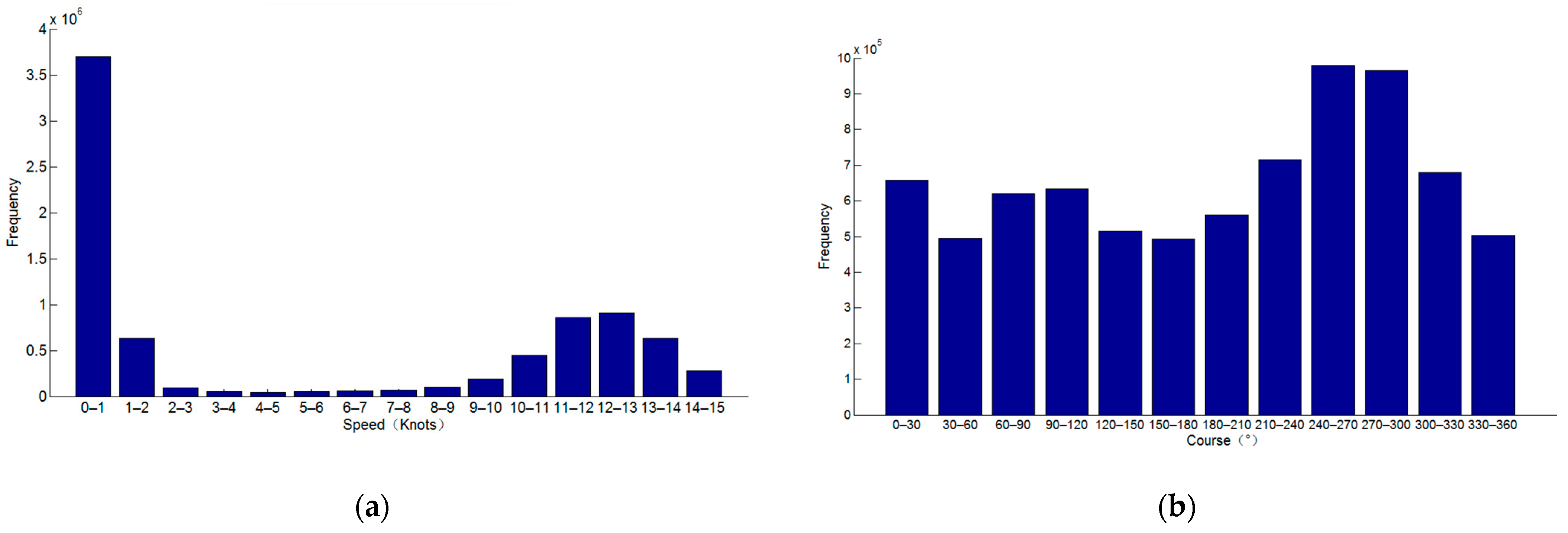
4.2. Speed and Heading Characteristics of Vessels

Figure 3 shows the velocity and course distribution of all position points of tuna purse seiners in this study. The interval distribution diagram of the tuna purse seine vessel’s speed and the course shows that speed exhibits a bimodal distribution, with the speed of most vessel position track points between 0 and 2 knots, and the other peak between 11 and 14 knots. The course distribution of tuna purse seiners is relatively uniform without marked characteristics. The speed of tuna purse seiners has distinct characteristics; however, the heading has no distinct characteristics.
Based on the bimodal distribution of the speed of tuna purse seiners, the speed is divided into two sections. The first interval is 0–2.5 knots, which corresponds to the tuna purse seiners harvesting nets. The second interval is 6–15 knots, corresponding to the high-speed transiting of tuna purse seiners to find or chase fish schools and set the net. Therefore, speeds of 0–2.5 knots and 6–15 knots can be used as speed thresholds to classify the operating status of tuna purse fishing vessels.

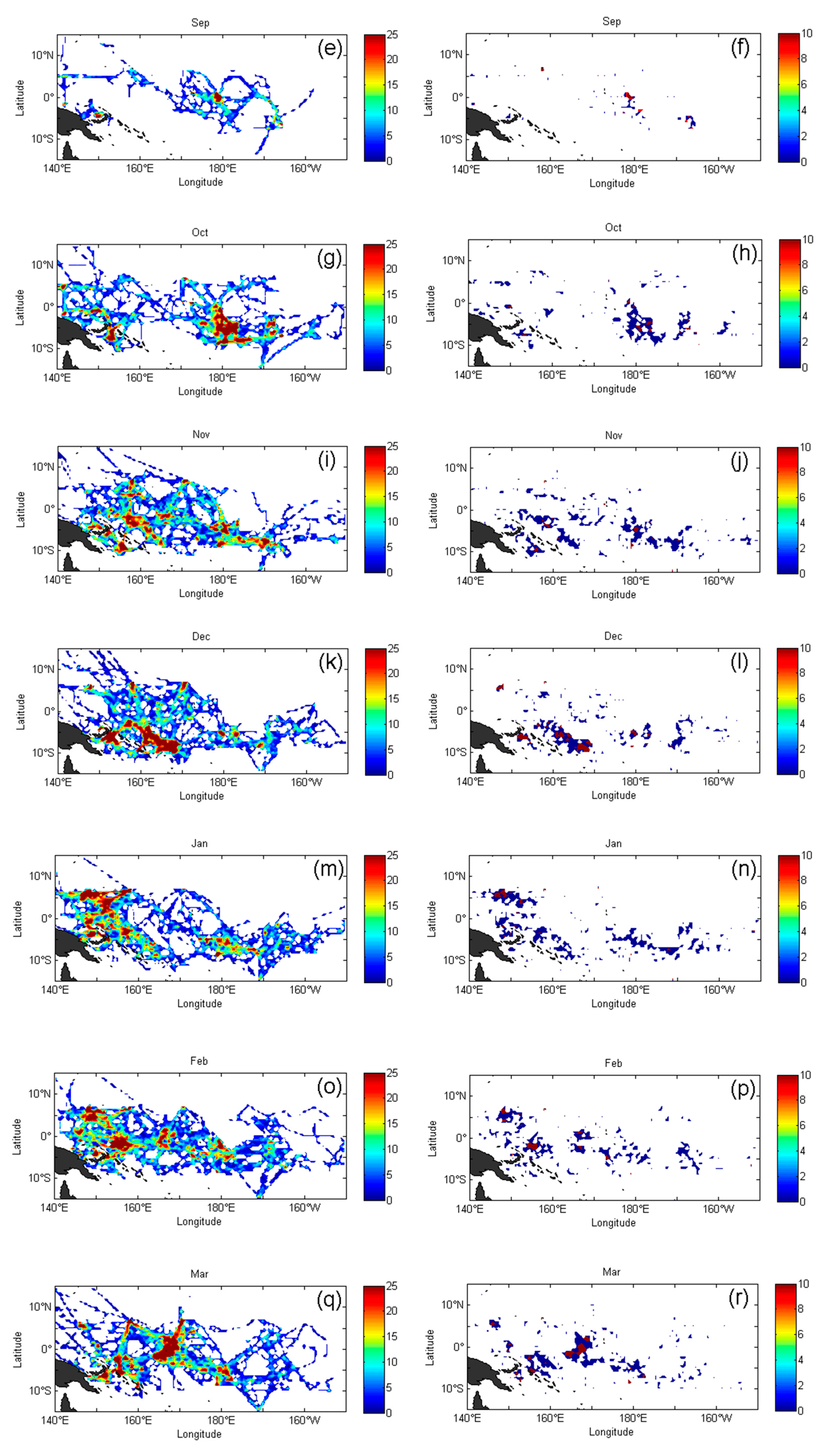
4.3. Distribution of Fishing Effort of Vessels in Each Month

Figure 4 is a time series diagram of the monthly fishing effort of 130 tuna purse seine vessels.
Compared with the broken line of purse seine operations, the accumulated time of high-speed transiting to find fish schools is longer than that of low-speed purse seine operation. Compared with the polyline that includes all vessel activities, the sum of the cumulative duration of high-speed transiting and low-speed purse seine operations is lower than the cumulative total duration of all vessel activities. Additionally, there were more vessel activities from October to December 2017 and January to May 2018 than from July to October 2017, and the cumulative total duration of the vessel locations was typically relatively large. Among these results, the total duration of the three types of data in September 2017 was the smallest compared to other months (i.e., vessels were less active in September 2017).
Figure 5 is a time series diagram of the coverage area of the vessel’s trajectory in each month. Based on the month, the 0.5° × 0.5° grid number under the fishing trajectory is added to describe the coverage area. The black broken line represents the coverage area of vessels under all actions, including high-speed transiting and collecting nets for fishing. The average monthly coverage rate is 27.2%. The broken red line represents the coverage area of the trajectories of vessels transiting at high speeds looking for fish or chasing fish, and the monthly average coverage rate is 26.9%. The broken blue line represents the coverage area of the trajectory of the vessel during low-speed purse seine operations, and the monthly average coverage rate is 7.1%. The coverage area of high-speed transiting and all behaviour states of vessels is similar, while the coverage area of purse seine operations is smaller.

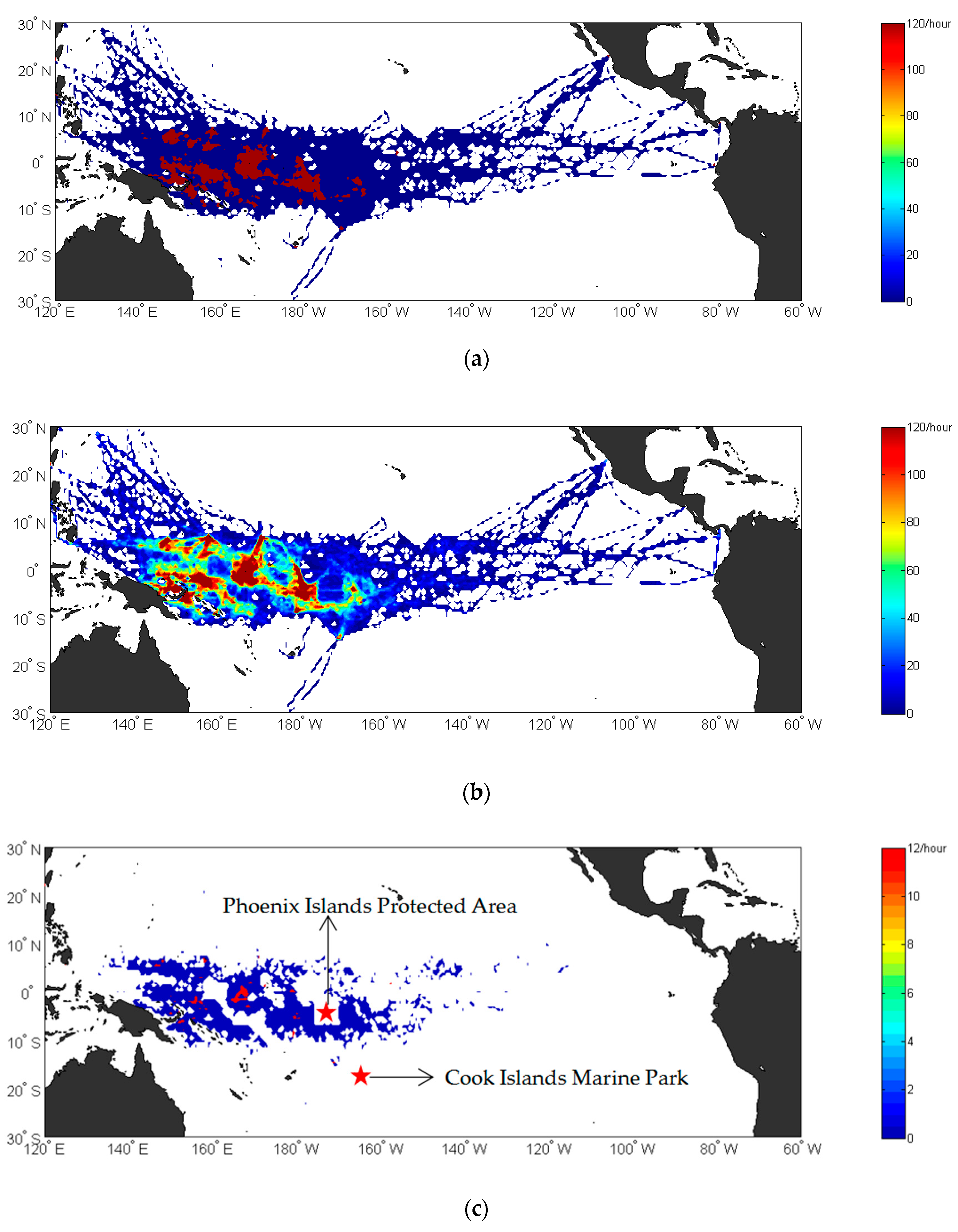
4.4. Spatial Analysis of Fishing Intensity of Vessels

Figure 6 shows the spatial distribution of fishing intensity of vessels in the Pacific Ocean 120° E–60° W, 30° S–30° N for 11 months from July 2017 to May 2018. The spatial resolution in this study is 0.5° × 0.5°.
Figure 6b shows that there are 3 areas where the time spent searching for fish schools is high. In each grid area, the time spent searching for fish schools for tuna purse seines exceeds 100 h. Off Papua New Guinea, the intensity of tuna purse seine fishing and the time spent by vessels looking for fish are large and located in an area where tuna purse seine vessels operate in high densities in the Western and Central Pacific. The area near 180° E east longitude and 10° S south latitude is the second area that shows high fishing intensity and high investment time for finding fish. The third high-intensity area for finding fish is near the equator (160° E–175° E east longitude), which corresponds to the high-intensity area of time investment in Figure 6a. These areas are consistent with the purse seine fishing operation area in Figure 6c. Tuna purse seine fishing operations are primarily distributed near the equator and south of the equator to 15° S latitude.
The study area includes an island located in the mid-western Pacific Ocean, the Phoenix Islands Protected Area between Hawaii and Fiji in the South Pacific, which have an area of approximately 408,250 km2. Additionally, there is a larger marine reserve called the Cook Islands Marine Park in the Pacific Ocean at 20° S south latitude and 165° W western longitude, which has an area of approximately 1,065,000 km2. Based on Figure 6c, the trajectory area involved in the fishing operation of the vessel does not cover the marine protected area, indicating that the fishing behaviour of the vessels is reasonable and standardized.
Based on Figure 1 and Figure 6, fishing operations and high-speed transiting are concentrated in the Pacific Ocean 140° E–150° W, 15° S–15° N. Next, we further discuss the characteristics of the trajectory and spatial distribution of vessels in these areas.
Figure 7 shows the spatial distribution of the fishing effort invested by tuna purse seine vessels with a 0.5° × 0.5° accuracy of searching for fish schools and purse seine every month. The spatial distribution map of vessels at 6–15 knots (i.e., high-speed transiting in search of fish during the day) is shown on the left side of Figure 7, and the spatial distribution map of vessel locations at 0–2.5 knots (i.e., seine fishing during the day) is shown on the right side of Figure 7. There are marked spatial differences in areas where tuna purse seine vessels search for fish stocks, and fishing operations are shown to be intense every month.
Figure 7a shows the images from July to December 2017, which shows vessels searching for fish in July was taken south of the equator between 150° E east longitude and 170° W west longitude. There are 4 high-intensity areas for finding fish, which are evenly distributed but small in area. The overall grid coverage rate is 20.1%, and the total time invested in the grid area of the tuna purse seine to search for fish schools reached 12,105 h. Figure 7b corresponds to a relatively discrete distribution of seine operating points. The primary concentrated area corresponds to the high-intensity area of fish hunting in Figure 7a. The grid coverage rate is 3.8%, and the time spent on purse seine fishing is approximately 5176 h. Figure 7c of finding fish in August is similar to that in July; however, the two high-intensity areas for finding fish near 165° E and 180° E longitude tend to expand north-south with a grid coverage of 17.6%. Additionally, the total time invested in finding fish schools equalled 10,414 h. Figure 7d of purse seine fishing operations has a corresponding expansion trend compared to that of Figure 7b. The grid coverage rate is 3.8%, and the total time of purse seine fishing operations equals 6015 h. In September, Figure 7e of finding fish and Figure 7f of purse seine fishing operations are located near the equator at 180° E east longitude. There is a marked high-intensity fish-finding area and a high-intensity fishing area. The grid coverage is 13.5% and 2.2%, and the total investment times are 5830 and 3604 h, respectively.
Looking for fish school Figure 7g in October, there are two primary high-intensity areas for finding fish in the latitude area from the south of the equator to the 15° S latitude, which are in the vicinity of 150° E east longitude and 180° E east longitude. The high-intensity area of fish hunting near 180°E is larger and corresponds to the area distribution in Figure 7h of its purse seine fishing operation. The grid coverage of Figure 7g,h are 27.6% and 6.9%, respectively, and the total time spent on fish hunting and purse seine operations are 17,251 and 8287 h, respectively. The high-intensity areas for finding fish school Figure 7i in November are relatively scattered and distributed in the latitude area from 5° N to 10° S and the longitude area from 150° E to 170° E. The grid coverage rate is 31.6%, and the total investment time for finding fish schools is 20,713 h. The area shown in the purse seine fishing operation Figure 7j corresponds to the distribution of the high-intensity fish-finding area in Figure 7i. Among these areas, there are two high-intensity fishing areas at 160° E and 180° E east longitude, and the grid coverage rate is 9.1%. The total fishing time is 11,242 h. Looking at the fish Figure 7k in December, there is a large high-intensity area for finding fish in the latitude area from south to 10° S of the equator and the longitude area from 150° E to 170° E. The high-intensity fishing area in Figure 7l is contrasted with this area. Its grid coverage for fish hunting and purse seine fishing is 31.5% and 7.7%, respectively, and the investment times are 20,648 and 11,395 h, respectively.
Analysing the images from January to May 2018, looking for fish in Figure 7m at 10° N to 10° S latitude area and 140° E–160° E east longitude, and 10° S south of the equator and 180° E east longitude in January, there are marked scattered areas with high intensities for fish hunting. In this image, the grid coverage rate is 30.4%, and the total investment time for finding fish schools is 20,935 h. In Figure 7n of purse seine fishing, there is a high-intensity fishing area near 5° S south latitude and 150° E east longitude. Compared with the fishing image of December 2017, the high-intensity fishing area near 10° S south latitude disappeared, and the area in the fish cluster changed. The image grid coverage of purse seine operations in January is 9.6%, and the total fishing investment time is 12,600 h. In February, looking for fish in Figure 7o, a high-intensity fishing area located near the equator and east longitude 165° E–170° E occurred in January. The overall search for fish trajectory area is more concentrated, the grid coverage rate is 32%, and the total investment time for finding fish schools is 21,123 h. In Figure 7p, the high-intensity area for purse seine operations is similar to the high-intensity area for fish hunting, the grid coverage rate is 8.8%, and the total fishing investment time is 10,103 h. In March, in the fish hunting as show in Figure 7q, the high-intensity fish hunting area was originally located near the equator and east longitude 165° E–170E but expands to the north-south direction, and the other high-intensity fish hunting areas decrease in intensity. The grid coverage rate is 31.5%, and the total investment time for finding fish is 21,706 h. In Figure 7r of purse seine operations, there is a marked high-intensity fishing area located near the equator at longitude 165° E–170° E east. The grid coverage rate is 8.8%, and the total fishing investment time is 12,932 h. In April in Figure 7s, the fish-finding high-intensity area near the equator and east longitude 165° E–170° E continues to expand along the east-west direction. The high-intensity fishing area in purse seine operation Figure 7t also increases in size accordingly. The grid coverage of the fish hunting and fishing images is 29.2% and 8.5%, respectively, and the investment times are 20,152 and 11,871 h, respectively. In May in the fish hunting Figure 7u, the high-intensity fish hunting areas are primarily concentrated from 5° S to 5° N and 140° E–170° E. However, the high-intensity fish hunting area near the equator and east longitude 165° E–170° E decreases, the grid coverage rate is 30.9%, and the total time for fish hunting is 21,894 h. In Figure 7v of purse seine operations, the high-intensity fishing area originally located in Figure 7t decreases, the grid coverage rate is 9.2%, and the total fishing investment time is 10,628 h.

4.5. Hot Spot Analysis of Vessels Fishing Intensity

4.5.1. Global Spatial Autocorrelation

During the 11 months from July 2017 to May 2018, we calculated a series of parameters, such as the mean, skewness, kurtosis, coefficient of variation, and global Moran’s I, for fishing intensity grid data for high-speed transiting and purse seine operations. The results are shown in Table 1 and Table 2.
In Table 1, the fishing effort invested in finding fish stocks from January to May of 2018 was typically greater than that in the second half of 2017. The skewness value of all months is greater than zero, indicating that the distribution is positive. The kurtosis values are much greater than 3, indicating that the fishing effort of the Pacific tuna purse seine vessels in search of fish schools is strongly concentrated in each month. The global Moran’s I index for all months is positive, the Z score is large, and the p value is zero; thus, fish hunting efforts in all months exhibit a concentrated distribution pattern. Additionally, the Z scores from March to May 2018 are particularly large; thus, the concentration of high-intensity areas for fish hunting in these months is marked.
In Table 2, the average fishing effort of purse seine is much higher than the average fishing effort of finding fish schools. The global Moran’s I indices in July, August, and September of 2017 were negative; the Z scores were smaller; and the p values were larger; thus, the fishing efforts in these three months showed a discrete distribution. In the other months, the Moran’s I index is positive, and the fishing effort shows a concentrated distribution. The Z scores are small and the p values are not zero; thus, the concentration of fishing effort is small. Additionally, in October 2017, the p values of January, February, and April of 2018 were relatively small, and the Z scores were above those of other months; thus, the fishing efforts in these months were more concentrated.

4.5.2. Hot Spots Distribution of Fishing Intensity

The results of the hot-spot analysis of fishing effort invested by vessels high-speed transiting are shown in Figure 8 for all 0.5° × 0.5° grids in this area of 140° E–150° W, 15° S–15° N. The hot spot area is similar to the area for finding fish clusters and purse seine operations in the spatial analysis of vessel fishing intensity.
There are multiple hot spots that are marked with a z value greater than 1.96, which indicates that the effort to find a school of fish in this area is large and is surrounded by high values. This area has strong spatial autocorrelation and positive correlation, and other areas are randomly distributed with z-values between −1.96 and 1.96. The spatial autocorrelation between high and low fish hunting efforts in these areas is weak, and the distribution is random.

4.6. Correlation Analysis

The correlation coefficients r 1 , r 2 and r 3 between the tuna purse seine production, net times, CPUE data and the fishing intensity invested by vessels high-speed transiting in the Western and Central Pacific are shown in Table 3. In 2017 and 2018, all correlation coefficients r > 0 ; thus, the data are positively correlated.
In July, October, November, and December of 2017 and in January, March, April, and May of 2018, r 1 > 0.8 ; thus, the output data of these months are highly correlated with the fishing intensity of looking for fish. Except for November 2017, r 2 > 0.8 in all other months, indicating a generally high correlation between the data of tuna purse seine nets in the Western and Central Pacific and the fishing intensity for finding fish stocks. For the correlation coefficient between the CPUE data of tuna purse seine nets in the Western and Central Pacific and the fishing intensity of looking for fish schools, 0.3 < r 3 < 0.8 is satisfied in each month; thus, there is a moderate correlation between the CPUE data and the fishing intensity of looking for fish schools.
Concurrently, the production, net times, CPUE data and fishing intensity for finding fish schools of tuna purse seine in the Western and Central Pacific Oceans satisfy the following linear regression equations:
Y 1 = 398.849 + 6.628 X
Y 2 = 9.657 + 0.245 X
Y 3 = 3.137 + 0.021 X

5. Discussion

5.1. Space Behaviour of a Single Vessel

The interval speed statistics observed indicate that (1) the operating speed of the tuna purse seine vessel exhibit marked changes, (2) that fishing behaviour is primarily described by vessel speed and 93) that heading characteristics are not clear.
Fishing vessel activity including transiting, searching for fish, fishing operations, and transshipment (Global Fishing Watch, 2019). Transshipment is very little compared to other behaviors; in the case of the tuna purse seine fishery, their main two fishing tactics. First, vessels detect free-swimming schools depends upon visual clues (birds, radars, and sonars). This means the vessel is searching for fish schools and the individual searching path of a vessel may be used to fishing effort [20]. Another fishing tactic is that the vessel directly sailing to the floating objects or artificial manmade fish aggregating devices (FADs), to find out if there was an association with a tuna school. This behavior means that the tuna purse seiner vessel moves quickly through abundance-poor areas and towards fishing grounds, which was indicated by the fish aggregating devices (FADs) or natural objects. These” cruising” phases were associated with high speeds.
On the other hand, if the tuna schools were found associated with the floating objects or FADs, the skippers try to track schools immediately. The instantaneous speeds of vessel are large while tracking. In this case, the tuna purse seiners vessel action was split into cruising, tracking, and fishing based on speed and turning angles [4]. It is worth mentioning that visual checking of tuna schools is constant on board fishing vessels during daylight, so that cruising phases have to be considered as effectively contributing to fishing effort, that is, searching for a tuna fishing school (effective in terms of detection of new, rich patches) [4]. Based on the above description, the vessel is sailing is considered as searching for fish schools. High speed was defined as searching/cruising and tracking. Finally, the purse seiners set the net to catch fish while the speed remains still. Therefore, the speed lower than 2.5 knots was defined as fishing operation in this paper and Souza [16] proved the accuracy as above.
For a single characteristic vessel, the operation trajectory diagrams analysed (speed and the fishing effort) give a good indication of the operating characteristics of the tuna purse seine vessel: high-speed transiting is used to find fish and sailing at low speed is used during fishing operations.

5.2. Distribution of Fishing Effort by Month

For the monthly fishing effort time series chart (Figure 4), the various broken lines show that it takes a long time for a tuna purse seine vessel high-speed transiting to find a school of fish. Once a tuna purse seine finds a school of fish, it will start fishing operations at a low speed or stop moving forward. The operation time depends on the catch, and the cumulative length of stay of various vessel activities is far greater than the sum of the cumulative duration of finding fish schools and purse seine operations. These phenomena likely occur because fishermen typically look for fish schools and perform fishing operations during the day, and a considerable amount of time occurs at night while fishermen rest, which is characteristic of tuna purse seine fishing. The grid number sequence diagram summarized in each month (Figure 5), describes the number of grids staying in each state of the vessel based on the characteristics of various broken lines.
According to our results, whether high-speed transiting or harvesting nets, the overall fishing intensity was below that in other months. David A. Kroodsma et al. [11] analysed the reasons for regular changes in the fishing effort of fishing boats. For non-Chinese vessels, the largest factor is Christmas holidays and weekends, while the annual pattern of Chinese vessels is primarily determined by the fishing moratorium during the Spring Festival and summer months.

5.3. Spatial Distribution Characteristics of Fishing Effort in Each Month

In the Pacific 140° E–150° W, 15° S–15° N area where vessels stay concentrated, we discuss the spatial distribution characteristics of fishing effort. This paper studies the spatial distribution of the fishing intensity of the tuna purse seine vessels for 11 consecutive months. There are marked differences in the space for transiting activities and fishing operations of tuna purse seine vessels in each month. The two types of images in the same month have highly corresponding distribution characteristics in space. Yuan Zuohui et al. [10] analysed the spatial distribution of tuna longline fishing intensity from July to December 2017 and found that there are multiple central fishing grounds in each month that tend to expand north–south, spread or shrink to varying degrees.
When the resolution of the image grid is small, real operating points are discrete, and the area involved in active fishing operations is small [21,22]. To facilitate observation, the grid resolution in this study is 0.5° × 0.5°. Nicolas Bez et al. [4] analysed the variance in various vessel activity grid data at different spatial resolutions, and the results showed that when the spatial resolution was 0.5° × 0.5°, the variance gradually showed a stable trend. Therefore, it is reasonable to use 0.5° × 0.5° as the spatial resolution to analyse the spatial characteristics of fishing intensity in this study.
Based on Moran’s I index, kurtosis, coefficient of variation and other statistical parameters in the global spatial autocorrelation analysis, we can obtain the spatial distribution of fishing intensity with a grid resolution of 0.5° × 0.5°, presenting a distinction between looking for fish schools and fishing operations. The coefficient of variation Cv is typically high, indicating that the fish resource density in each grid area is different. The coefficient of variation in fishing operations in this study is much higher than that of looking for fish schools, which again confirms the features of the operation mode. The statistical results of other types of spatial parameters show that the fishing intensity for looking for fish schools occur in a concentrated distribution pattern, and the real fishing intensity presents a relatively discrete distribution pattern, which is consistent with the operating characteristics of tuna purse seine vessels. Yang Xiaoming et al. [23] used spatial statistical methods to analyse bonito purse seine fishing in the Western and Central Pacific and found that bonito resources in the Western and Central Pacific showed a strong agglomeration and distribution as calculated by the hot-spot analysis method of local spatial autocorrelation. They also found that local spatial autocorrelation was strong.

5.4. Enlightenment of Fishing Effort to Resources

This paper examines the correlation between the defined fishing effort and the obtained tuna purse seine catch data. The fishing effort of each month is highly correlated with the output and net times data, and the CPUE data are moderately correlated. The proposed one-variable linear regression model described the linear relationship between fishing effort and production, net times, and CPUE data. Without considering error, the real output, real net times and real CPUE can be estimated based on the length of stay of the vessels in the grid. We used the behaviour of the vessels to directly and roughly infer the biomass level in its population. Bertrand et al. [24] simulated the trajectory of vessels via a random walk model, and results showed that the spatial behaviour of vessels is essentially the same as predator behaviour.
Traditional fishery data faces several difficulties to describe various behaviours of vessels in a timely and effective manner. This study uses AIS data to analyse the behaviour of tuna purse seine vessels in the Western and Central Pacific. The definition of fishing effort in this study can be used to investigate the distribution of resources; for example, based on vessel behaviour, the location of the fish school can be estimated, and the distribution of fish clusters and fishing grounds can be predicted. Cimino et al. [12] combined the behaviour of vessels with information on ocean conditions and explored the relationship between fishing behaviours and environmental factors. The area in the fish cluster is related to environmental factors, that is, the spatial behavior of the vessel is closely related to the marine environment. Future research should consider environmental factors, analyse the geographic distribution of marine environmental factors, link these factors to the fishing effort of vessels, and explore the contribution of marine environmental factors to the behaviour of vessels.

Author Contributions

Conceptualization, H.Z. and S.-L.Y. (Sheng-Long Yang); methodology, H.Z. and H.-M.S.; software, H.Z. and H.-M.S.; validation, S.-L.Y. (Sheng-Long Yang) and W.F.; formal analysis, S.-L.Y. (San-Ling Yuan) and W.F.; data curation, H.Z., and S.-L.Y. (Sheng-Long Yang); writing—original draft preparation, H.Z.; writing—review and editing, S.-L.Y. (Sheng-Long Yang) and H.-M.S.; validation, W.F. and S.-L.Y. (San-Ling Yuan); visualization, H.Z.; supervision, S.-L.Y. (San-Ling Yuan) and S.-L.Y. (Sheng-Long Yang); project administration, S.-L.Y. (San-Ling Yuan), W.F. and S.-L.Y. (Sheng-Long Yang). All authors have read and agreed to the published version of the manuscript.

Funding

This research was funded by the National Natural Science Foundation of China (12071293), the National Key R&D Program of China (2019YFD0901404,2019YFD0901405), the Special Funds of Basic Research of Central Public Welfare Institute (2019T09), Shanghai Science and technology innovation action plan (19DZ1207504), Scientific Research Program of Shanghai Science and Technology Commission (18391900800), Jimei University, Fujian Provincial Key Laboratory of Marine Fishery Resources and Eco-environment and Fujian Provincial Key Laboratory of Marine Fishery Resources and Eco-environment Funding (fjmfre2019003).

Institutional Review Board Statement

Not applicable.

Informed Consent Statement

Not applicable.

Data Availability Statement

Publicly available datasets MMSI number were analyzed in this study. This data can be found here: https://docs.qq.com/sheet/DQ0FQTnJuVHhBSGhJ, accessed on 14 March 2021.

Acknowledgments

The authors of this research would like to thank all the researchers who contributed to the research process during our study, and the data provided by Global Fishing Watch Data.

Conflicts of Interest

The authors declare no conflict of interest.

References

  1. Xie, Y.L. Status and prospects of tuna fisheries in the Western and Central Pacific. Mod. Fish. Inf. 2002, 9, 18–20. [Google Scholar]
  2. Lee, J.; South, A.B.; Jennings, S. Developing reliable, repeatable, and accessible methods to provide high-resolution estimates of fishing-effort distributions from vessel monitoring system (VMS) data. Ices J. Mar. Sci. 2010, 67, 1260–1271. [Google Scholar] [CrossRef] [Green Version]
  3. Martín, P.; Muntadas, A.; de Juan, S.; Sánchez, P.; Demestre, M. Performance of a northwestern Mediterranean bottom trawl fleet: How the integration of landings and VMS data can contribute to the implementation of ecosystem-based fisheries management. Mar. Policy 2014, 43, 112–121. [Google Scholar] [CrossRef]
  4. Bez, N.; Walker, E.; Gaertner, D.; Rivoirard, J.; Gaspar, P. Fishing activity of tuna purse seiners estimated from vessel monitoring system (VMS) data. J. Fish. Aquat. Sci. 2011, 68, 1998–2010. [Google Scholar] [CrossRef]
  5. Piet, G.J.; Hintzen, N.T. Indicators of fishing pressure and seafloor integrity. Ices J. Mar. Sci. 2012, 69, 1850–1858. [Google Scholar] [CrossRef]
  6. Murray, L.G.; Hinz, H.; Hold, N.; Kaiser, M.J. The effectiveness of using CPUE data derived from Vessel Monitoring Systems and fisheries logbooks to estimate scallop biomass. Ices J. Mar. Sci. 2013, 70, 1330–1340. [Google Scholar] [CrossRef] [Green Version]
  7. Shepperson, J.L.; Hintzen, N.T.; Szostek, C.L.; Bell, E.; Murray, L.G.; Kaiser, M.J. A comparison of VMS and AIS data: The effect of data coverage and vessel position recording frequency on estimates of fishing footprints. Ices J. Mar. Sci. 2018, 75, 988–998. [Google Scholar] [CrossRef]
  8. McCauley, D.J.; Woods, P.; Sullivan, B.; Bergman, B.; Jablonicky, C.; Roan, A.; Hirshfield, M.; Boerder, K.; Worm, B. Ending hide and seek at sea. Science 2016, 351, 6278. [Google Scholar] [CrossRef] [Green Version]
  9. Yang, S.L.; Zhang, S.M.; Yuan, Z.H.; Dai, Y.; Zhang, H.; Zhang, B.B.; Fan, W. The fishing intensity calculation of ocean longline fishing grounds based on the fishing behavior characteristics of vessels. J. Fish. Sci. China 2020, 27, 307–314. [Google Scholar]
  10. Yuan, Z.H.; Yang, D.H.; Fan, W.; Zhang, S.M. Research on the distribution of tuna longline fishing grounds in the Western and Central Pacific based on satellite AIS. Mar. Fish. 2018, 40, 649–659. [Google Scholar]
  11. Kroodsma, D.A.; Mayorga, J.; Hochberg, T.; Miller, N.A.; Boerder, K.; Ferretti, F.; Wilson, A.; Bergman, B.; White, T.D.; Block, B.A.; et al. Tracking the global footprint of fisheries. Science 2018, 359, 6378. [Google Scholar] [CrossRef] [Green Version]
  12. Cimino, M.A.; Anderson, M.; Schramek, T.; Merrifield, S.; Terrill, E.J. Towards a Fishing Pressure Prediction System for a Western Pacific EEZ. Sci. Rep. 2019, 9, 1. [Google Scholar] [CrossRef] [PubMed]
  13. Qi, J.J.; Wang, M.Y. The current status and prospects of the world tuna purse seine fishery. Mar. Fish. 2001, 10, 18–20. [Google Scholar]
  14. Tang, F.H.; Cui, X.S.; Yang, S.L.; Zhou, W.F.; Cheng, T.F.; Wu, Z.L.; Zhang, H. GIS Spatiotemporal Analysis of the Impact of Marine Environment on the Western and Central Pacific Ocean Tuna Purse Seine Fishing Grounds. South. Fish. Sci. 2014, 10, 18–26. [Google Scholar]
  15. Li, S.G. Study on the Operating Characteristics and Safety of Purse Seine Vessels; Dalian Maritime University: Dalian, China, 2010. [Google Scholar]
  16. de Souza, E.N.; Kristina, B.; Stan, M.; Boris, W. Improving Fishing Pattern Detection from Satellite AIS Using Data Mining and Machine Learning. PLoS ONE 2016, 11, e0158248. [Google Scholar]
  17. Lamigueiro, O.P. solaR: Solar Radiation and Photovoltaic Systems with R. J. Stat. Softw. 2012, 50, 9. [Google Scholar]
  18. Kalogirou, S. Spatial autocorrelation (Catmog47); Geo Books: Nowich, UK, 1986. [Google Scholar]
  19. Mitchell, A. The ESRI Guide to GIS Analysis; ESRI Press: California, CA, USA, 2005; Volume 2. [Google Scholar]
  20. Polacheck, T. Analyses of the relationship between the distribution of searching effort, tuna catches, and dolphin sightings within individual purse seine cruises. Fish. Bull. 1988, 86, 351–366. [Google Scholar]
  21. Clark, T.P.; Longo, S.B. New Findings from University of Washington Update Understanding of Science (Comment on “Tracking the global footprint of fisheries.”). Sci. Lett. 2018, 60, 225–248. [Google Scholar]
  22. Kroodsma, D.A. Response to Comment on “Tracking the global footprint of fisheries”. Sci. Lett. 2018, 361, eaat7789. [Google Scholar] [CrossRef] [Green Version]
  23. Yang, X.M.; Dai, X.J.; Tian, S.Q.; Zhu, G.P. Hot spot analysis and spatial heterogeneity of bonito purse seine fishery resources in the Western and Central Pacific Ocean. Acta Ecol. Sin. 2014, 34, 3771–3778. [Google Scholar]
  24. Bertrand, S.; Bertrand, A.; Guevara-Carrasco, R.; Gerlotto, F. Scale-invariant movements of fishermen: The same foraging strategy as natural predators. Ecol. Appl. 2007, 17, 2. [Google Scholar] [CrossRef] [PubMed]
Figure 1. Study area: the spatial track points involved a total of 130 vessels (red area: the position of the vessels; blue area: the land).
Jmse 09 00322 g001
Figure 2. Track characteristics of a single vessel: (a) The vessel trajectory velocity from January to May 2018; (b) The vessel trajectory velocity from April 15 to 30; (c) The spatial diagram of fishing intensity from January to May 2018; (d) The spatial diagram of fishing intensity from April 15 to 30.
Jmse 09 00322 g002
Figure 3. Interval distribution of speed and course: (a) Interval distribution of speed; (b) Interval distribution of course.
Jmse 09 00322 g003
Figure 4. Time series chart of fishing effort by month: (1) The black broken line: the time invested by the vessels in all actions, including high-speed transiting and collecting nets for fishing; (2) The broken red line: the amount of fishing effort invested by the vessel transiting at high-speed to find or chase the fish; (3) The broken blue line:the amount of fishing effort invested by the vessels during low-speed purse seine operations.
Jmse 09 00322 g004
Figure 5. Summary of the number of grids: The color of the broken line in the figure indicates the same meaning as in the Figure 4.
Jmse 09 00322 g005
Figure 6. Overall spatial distribution of fishing effort: (a) All behaviour of vessels; (b) high-speed transiting: looking for or chasing fish schools; (c) purse seine operations. (: Marine Protected Area).
Jmse 09 00322 g006
Figure 7. Spatial distribution of fishing effort intensity:(a,c,e,g,i,k,m,o,q,s,u) high-speed transiting in search of fish during the day; (b,d,f,h,j,l,n,p,r,t,v) seine fishing during the day. The color bar refers to the duration of stay of vessels, and the unit is hour.
Jmse 09 00322 g007aJmse 09 00322 g007bJmse 09 00322 g007c
Figure 8. Hot spots analysis of fishing effort invested by vessels at high-speed transiting (Hot spots = red areas; based on 0.5° × 0.5° grids).
Jmse 09 00322 g008
Table 1. Parameter statistics of the effort invested in high-speed transiting.
MonthMeanSDSkewnessKurtosisCv(S/m)S2/mMoran’s IZ Scorep
2017.077.0098.3564.02925.4961.1929.9580.43436.9630.000
2017.086.8839.2463.85920.9471.34312.4190.40243.2160.000
2017.095.0406.8675.72150.5201.3639.3560.36341.4280.000
2017.107.2739.2203.26314.2091.26811.6890.51892.9250.000
2017.117.6308.6193.39421.4281.1309.7350.17275.0190.000
2017.127.61110.8134.35929.1411.42115.3630.487112.5300.000
2018.018.0129.7983.42218.6501.22311.9810.36293.1780.000
2018.027.6708.8853.25417.0751.15810.2920.366119.2250.000
2018.038.01611.8604.73133.8891.48017.5500.261143.6490.000
2018.048.02211.8493.64817.0431.47717.5000.480210.1230.000
2018.058.22812.0894.12028.1791.46917.7610.243148.6280.000
Table 2. Parameter statistics of the effort invested in purse seine operation.
MonthMeanSDSkewnessKurtosisCv(S/m)S2/mMoran’s IZ Scorep
2017.0715.92981.5249.949107.1815.118414.249−0.004−0.1290.897
2017.0818.454106.11511.304141.1215.750610.198−0.0020.2040.839
2017.0918.87084.8737.95570.8024.498381.748−0.0020.1730.863
2017.1013.97585.76412.804190.9676.137526.3240.0051.0070.314
2017.1114.395100.71514.570240.5256.996704.6460.0020.6250.532
2017.1217.161104.20010.866123.1016.072632.6800.0010.5090.611
2018.0115.25597.52814.109242.1696.393623.5080.0041.0030.316
2018.0213.34782.98613.697210.5336.218515.9880.0071.1500.250
2018.0317.152110.03612.251163.5876.415705.9090.0020.8220.411
2018.0416.26298.95613.178196.6836.085602.1530.0031.1400.254
2018.0513.48896.47420.922501.5337.152690.0280.0000.3670.714
Table 3. Statistics of correlation coefficient.
YearMonthr1r2r3
201770.8500.8450.465
80.7890.8090.386
90.7730.8120.334
100.8710.8680.690
110.8700.7840.796
120.8430.8860.378
201810.8070.8790.590
20.7690.8220.596
30.8600.8010.591
40.8870.8630.617
50.8320.9010.504
Publisher’s Note: MDPI stays neutral with regard to jurisdictional claims in published maps and institutional affiliations.

