Daily Prediction of the Arctic Sea Ice Concentration Using Reanalysis Data Based on a Convolutional LSTM Network

Abstract

To meet the increasing sailing demand of the Northeast Passage of the Arctic, a daily prediction model of sea ice concentration (SIC) based on the convolutional long short-term memory network (ConvLSTM) algorithm was proposed in this study. Previously, similar deep learning algorithms (such as convolutional neural networks; CNNs) were frequently used to predict monthly changes in sea ice. To verify the validity of the model, the ConvLSTM and CNNs models were compared based on their spatiotemporal scale by calculating the spatial structure similarity, root-mean-square-error, and correlation coefficient. The results show that in the entire test set, the single prediction effect of ConvLSTM was better than that of CNNs. Taking 15 December 2018 as an example, ConvLSTM was superior to CNNs in simulating the local variations in the sea ice concentration in the Northeast Passage, particularly in the vicinity of the East Siberian Sea. Finally, the predictability of ConvLSTM and CNNs was analysed following the iteration prediction method, demonstrating that the predictability of ConvLSTM was better than that of CNNs.

1. Introduction

The Arctic is covered by sea ice throughout the year, which plays an important role in global climate regulation [1]. However, in recent decades, the area covered by sea ice in the Arctic has been declining. An increase in temperature causes the sea ice to melt, which then causes the sea surface albedo to decrease and solar radiation absorption to increase, and the temperature to continue to rise [2,3]. Changes in sea ice coverage affect the global transportation industry. For example, with the reduction of sea ice coverage, the possibility of navigation in the Arctic is gradually increasing. In particular, the Northeast Passage is becoming navigable in summer [4].

The potential utilization of the Arctic natural resources highlights the urgent need of sea ice prediction. Taking the waterway as an example, sea ice impedes the normal voyage of ships and the accurate prediction of sea ice is thus the premise of the safe navigation. However, due to the limitations of observational data and the highly non-linear dynamic changes of sea ice, sea ice prediction is still a difficult task. In addition, the sea ice prediction contains many factors. From the perspective of navigation in Arctic area, sea ice concentration (SIC) has a greater impact on ship safety [5]. Therefore, this study focuses on the prediction of SIC.

Both modeling and statistical studies are good tools for current sea ice prediction. For model simulation, the mainstream sea ice models, such as the Los Alamos sea ice model (CICE) and the Louvain-la-Neuve sea ice model (LIM) [6,7], are based on the known physical processes. Both thermodynamic and dynamic processes of sea ice evolution are considered, including temperature, salinity, melting pool, boundary layer momentum exchange, and sea ice ridging and rafting, etc.

Through the clear laws of physical change and considering a variety of factors that affect sea ice changes, the model prediction can give assimilation results with stable errors and strong interpretability. Most current large-scale sea ice processes are well analysed and sketched intuitively in the model [8]. However, some important details of sea ice dynamics and deformation have not been well portrayed, especially in small scales [8,9,10]. The development of the sea ice models mainly focuses on: (1) a more accurate description of the microstructure evolution and anisotropy of sea ice, (2) topics of study include biological and chemical species, (3) representation of thickness changes at the sub-grid scale, and (4) a redistribution mechanism that transforms thinner ice into thicker ice under deformation [8].

In addition, since the fifth assessment report of the Intergovernmental Panel on Climate Change (IPCC), a high-level understanding of the physical drivers of local changes in Arctic sea ice has been recognized. According to studies conducted by researchers, a variety of factors contribute significantly to the local sea ice cover such as temperature changes [11], humidity transport [12], wind field model [13], cloud cover [14], and ocean heat flux [15], etc. The main direction of the sea ice models development is how to use models to better describe these physical processes and to better couple them with the atmospheric and ocean models.

However, statistical prediction is based on the data itself without prior linear or nonlinear variation, which can make up for the deficiency of model prediction to some extent. A vector autoregressive model (VAR) was used to statistically predict the sea ice concentration in the Arctic during summer (May to September) [16]. However, to reduce the degree of freedom and calculation cost, the considered SIC spatial resolution is insufficient to use in practical applications, such as Arctic trajectory planning. The VAR and vector Markov models were used to establish a weekly SIC prediction model based on multiple sea ice, oceanic, and atmospheric factors [17]. The model could predict SIC for 3–6 weeks well; however, the root-mean-squared-error (RMSE) in summer was continuously high, at approximately 20%. Moreover, the conventional statistical algorithms can only build point-wise models, ignoring the interaction between neighboring points (so-called spatial correlation hereinafter).

In recent years, deep learning (DL) has been gradually applied to sea ice prediction and achieved certain results due to its excellent nonlinear fitting effect. A variety of DL-based works focus on improving the point-wise prediction. A monthly SIC prediction model based on a long short-term memory network (LSTM) that performed monthly autoregressive prediction based on the change law of the SIC itself [18]. The predictive effect of the model had been improved by incorporating information of the time dimension. A multi-model ensemble prediction method based on deep neural network, and used various climatic factors for SIC regression prediction [19]. Similar to conventional VAR algorithm, spatial correlation was not considered in the above two works. This problem was partly circumvented by [20], which included the “global information” into the point-wise DL model.

In fact, the spatial correlation can be well considered through the convolutional operation. CNNs was used to predict the SIC in the Gulf of St. Lawrence based on the observations of a synthetic aperture radar (SAR) [21]. Lawrence based on the observations of a synthetic aperture radar (SAR). Based on the SIC and other meteorological and oceanic factors, monthly CNNs was established to predict the SIC of the next month [22]. The main problem of CNNs lies in that the SIC of given time (t) is totally determined by (t-1). The “nearsightedness” of CNNs underscores the defect of conventional CNN in tackling temporal variation.

To the best of our knowledge, the application of DL technology in SIC prediction is mainly annual or monthly predictions. There has been little use of DL technology in daily prediction of SIC. However, the monthly prediction cannot meet the requirements of practical scientific or commercial operations. For example, it takes about 15 days for vessels to complete the Arctic voyage, which is in urgent demand of the daily predictions to evaluate and adjust daily routes [23]. Different from the monthly prediction, the daily prediction sets a formidable challenge for the statistical algorithms since the spatial correlation and temporal variation are much more highlighted in daily SIC.

Therefore, the aim of this study was to construct a reliable model of daily SIC prediction. The accuracy of daily SIC prediction was improved by introducing convolution calculation and considering the spatiotemporal variation of SIC. The remainder of this paper is structured as follows: Section 2 describes the data used, Section 3 describes the method and design of the experiment, Section 4 describes the results of the experiment, and Section 5 summarizes the whole paper.

2. Data

2.1. NSIDC Data

The SIC data used in this study were obtained from the National Snow and Ice Data Centre (NSIDC) and consisted of horizontally gridded data provided daily. The NSIDC data were synthesized by the Scanning Multichannel Microwave Radiometer (SMMR) of the Nimbus-7 satellite and Special Sensor Microwave/Imager (SSM/I) of the US Defense Meteorological Satellite Program (DMSP) [24]. This dataset provided researchers with the daily and monthly SIC in the Arctic and Antarctic regions, with a horizontal resolution of 25 × 25 km. After quality control and data correction of NSIDC, the value of SIC had been standardized to between 0 and 100%, except for missing values such as land.

NASA’s sea ice calculation team determines SIC based on the Climate Data Record (CDR) algorithm [25]. The output of this algorithm is a rule-based combination of ice concentration estimates from two well-established algorithms: the NASA Team (NT) algorithm [26] and the NASA Bootstrap (BT) algorithm [27]. The errors of the two algorithms are not the same. In winter when the temperature is very low, the results of the BT algorithm tend to underestimate the value of SIC [28]. While, in the winter when the temperature is relatively mild, the results of the NT algorithm tend to be lower [29]. Therefore, the final result of CDR algorithm is to take the maximum of the two algorithms [30]. According to research by NASA’s sea ice algorithm team, the accuracy of the SIC data in this dataset can reach ±5% in winter and ±15% in summer. The accuracy is highest when the sea ice thickness exceeds 20 cm [31].

In this study, data of the Northeast Passage region were selected from the SIC data of NSIDC, the SIC data from 2008 to 2017 were used as the training set, and the SIC data of 2018 were used as the true value to test the prediction effect of the subsequent models.

2.2. Data Preprocessing

SIC data from Nimbus-7 SMMR and DMSP SSM/I-SSMIS version 3 were used in this study. As this work focuses on the Northeast Passage, the selected SIC spatial coverage ranges were 65° N–83° N, 0°–180° E, and 165° W–180° W. In addition, 3653 days of data from 2008 to 2017 were used for model training, and 365 days of data for 2018 were used for model testing and effect verification. The research area was shown in Figure 1.

During the training of the CNNs and convolutional long short-term memory network (ConvLSTM), rather than processing the whole picture at once, the picture was divided into multiple small blocks to allow the convolution kernel to better detect the edge features of each patch when processing the image. This can also aid in regularization role, allowing fewer estimated parameters to be used to achieve better training results. Therefore, the study area was divided into 20 patches, and the original 205 × 188 dataset was divided into 41 × 47 × 20 before being used for the subsequent convolution neural network calculation. Additionally, as there can be no singular value in the convolution calculation, we set the Nan value of land as 0 in model training; therefore, the SIC was 0.

This study focused on the autoregression of SIC. CNNs and ConvLSTM were used to learn the changing law of SIC for short-term prediction, and the prediction effects of the two models were compared.

3. Methods

In this study, the most suitable model for daily SIC prediction was selected by comparing the prediction effect of the CNNs and ConvLSTM. The main factors are shown in Figure 2.

3.1. Convolutional Neural Networks (CNNs)

CNNs are a class of neural networks that include convolution calculations and have a deep structure, which were first proposed by [32]. CNNs were initially used for text recognition in documents, and with the development and improvement of networks, CNNs have been widely used in image recognition and classification [33,34].

CNNs can handle multi-dimensional data. The input layer of a one-dimensional network receives a one-dimensional or two-dimensional array, while the input layer of a two-dimensional network receives a two- or three-dimensional array. The CNNs used in this study were two-dimensional convolution calculations, and the input array was a three-dimensional array, i.e., height × width × channel (41 × 47 × 20).

The neurons in the adjacent convolution layer are not fully connected but are connected to multiple nearby neurons in the upper layer. The size of the connection area depends on the size of the convolution kernel; therefore, the size of the convolution kernel is also known as “receptive field” [35]. The convolution layer contains several convolution kernels, and the function of the convolution layer depends on the convolution kernel. The main parameters of the convolution kernel are the weight coefficient and bias vector. When the convolution kernel works, it regularly scans the input features. In the receptive field, the input features are multiplied by matrix elements, and the deviation is added. The two-dimensional convolution kernel is calculated as follows:

$$\begin{array}{c}{\mathit{Z}}^{l+1}(i,j)=\left[{\mathit{Z}}^l\otimes {\mathit{w}}^{l+1}\right](i,j)+\mathit{b}={\displaystyle {\displaystyle \sum }_{k=1}^{K_l}}{\displaystyle {\displaystyle \sum }_{x=1}^f}{\displaystyle {\displaystyle \sum }_{y=1}^f}\left[{\mathit{Z}}_k^l\left(s_{0}i+x,s_{0}j+y\right){\mathit{w}}_k^{l+1}(x,y)\right]+\mathit{b}\\ (i,j)\in \left\{0,1,\dots L_{l+1}\right\}\hspace{1em}{L}_{l+1}=\frac{L_l+2p-f}{s_0}+1\end{array}$$

(1)

The summation part of the above formula can be understood as the solution of a cross-correlation, where $\mathit{b}$ is the deviation; ${\mathit{Z}}^l$ and ${\mathit{Z}}^{l+1}$ represent the convolution input and output of the $l+1$ layer, also known as the feature map, respectively; $L_{l+1}$ is the size of ${\mathit{Z}}^{l+1}$, assuming that the height and width of the feature map are the same; $\mathit{Z}(i,j)$ is the pixel grid of the feature map; $K$ is the number of channels in the feature map; and $f$, $s_0$, and $p$ are convolutional layer parameters, which are also hyperparameters of CNNs that correspond to the size of the convolution kernel, convolution stride, and padding, respectively.

When the size of the convolution kernel is $f=1$, stride is $s_0=1$, and the filled unit convolution kernel is not included, the cross-correlation calculation in the convolution layer is equivalent to matrix multiplication, and a fully connected network can be constructed between the convolution layers. The calculation method was as follows:

$${\mathit{Z}}^{l+1}={\displaystyle \sum }_{k=1}^{K_l}{\displaystyle \sum }_{i=1}^L{\displaystyle \sum }_{j=1}^L\left({\mathit{Z}}_{i,j,k}^l{\mathit{w}}_k^{l+1}\right)+\mathit{b}={\mathit{w}}_{l+1}^T{\mathit{Z}}_{l+1}+\mathit{b},\hspace{1em}{L}^{l+1}=L$$

(2)

This convolution layer was used to replace the full connection layer in the traditional convolution neural network and generate a two-dimensional characteristic map of the SIC.

The hyper-parameters of the CNNs include the kernel, stride, and padding, which together determine the output size of the convolution layer. The specified size of the kernel can be any value smaller than the size of the input image. The larger the size of the kernel, the more complex the input features that can be extracted; however, more parameters would need to be trained in the corresponding kernel. The stride defines the distance between the positions of the kernel when it scans the feature map twice. When the stride is 1, the kernel will scan the elements of the feature map individually. The padding is typically divided into valid and the same padding. For valid padding, no padding is used, and the kernel only allows access to the position of the feature map that contains the complete receptive field; however, the size of the output feature map will gradually decrease. The same padding refers to the use of sufficient padding to keep the output and input feature maps at the same size. For this type of padding, the size of the feature map will not be reduced. The CNNs constructed in this study only used this padding method.

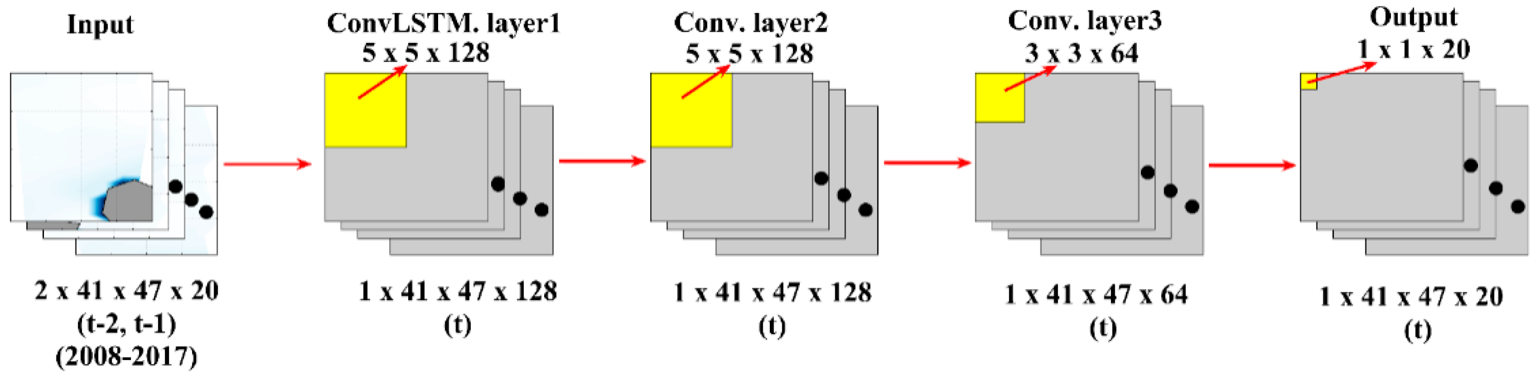
3.2. Convolutional Long-Short Term Memory Network (ConvLSTM)

ConvLSTM was initially developed from long short-term memory (LSTM). LSTM is a time-loop neural network based on recurrent neural networks (RNNs), and it is specially designed to solve the long-term dependence problem of general RNNs. RNNs and LSTM are mainly used in fields such as speech recognition, language modelling, text translation, and spatiotemporal positioning [36]. RNNs can learn to use previous information to predict subsequent information but can only consider information with a short time interval. As the time interval increases, RNNs lose their ability to learn distant information; thus, LSTM has improved in this regard [37].

LSTM can decide to remove or add information to a cell through a carefully designed “gate”, which is a selective information passing method, usually a sigmoid neural network layer. The output of this layer is a value between 0 and 1 that describes how much of each part can pass. A value of 0 means that no information can pass, and 1 means that all information can pass. LSTM usually contains three gate structures:

• Input gate, which decides how much information is inputted into the network. The inputted information is composed of the inputs at the previous moment and this moment.
• Output gate, which decides how much information is outputted to the next layer.
• Forget gate, which is the most critical gate and determines how much of the previous information is forgotten. This gate consists of the state value at the previous moment, input at this moment, and output at the previous moment.

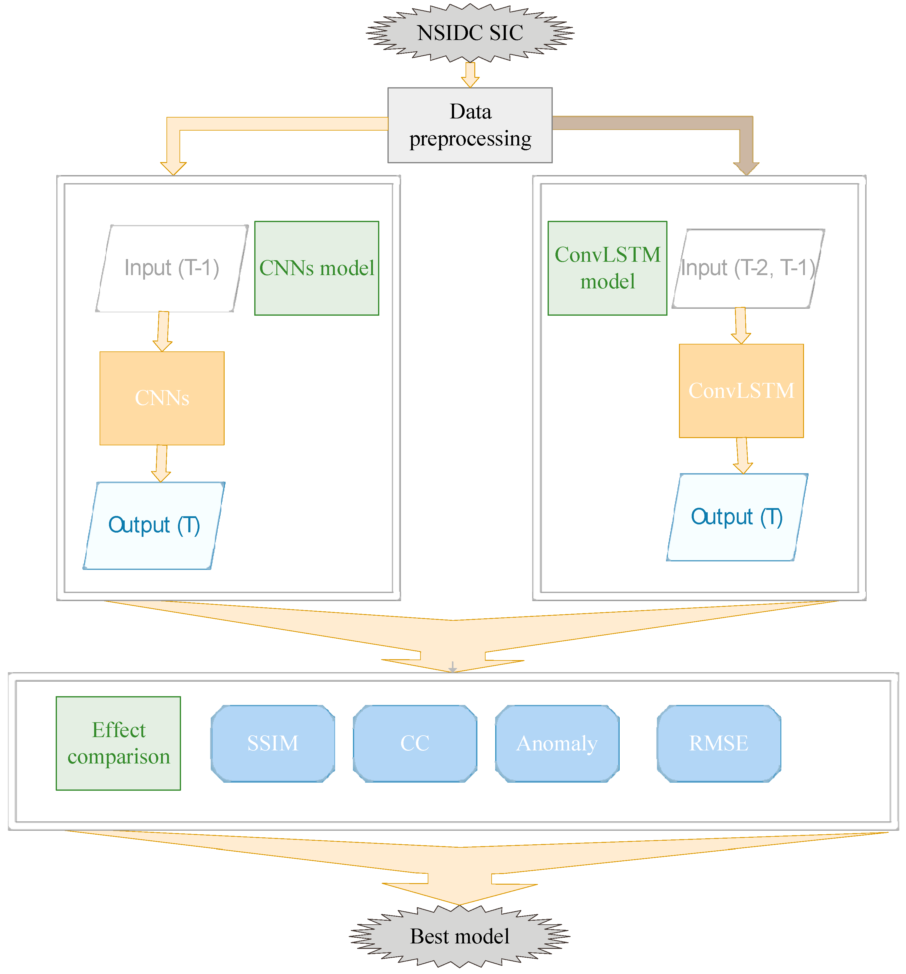
The main calculation process of LSTM is as follows:

$$\begin{array}{l}{i}_t=\sigma \left(W_{xi}{x}_t+W_{hi}{h}_{t-1}+W_{ci}\circ c_{t-1}+b_i\right)\\ f_t=\sigma \left(W_{xf}{x}_t+W_{hf}{h}_{t-1}+W_{cf}\circ c_{t-1}+b_f\right)\\ c_t=f_t\circ c_{t-1}+i_t\circ \tanh \left(W_{xc}{x}_t+W_{hc}{h}_{t-1}+b_c\right)\\ o_t=\sigma \left(W_{xo}{x}_t+W_{ho}{h}_{t-1}+W_{co}\circ c_t+b_o\right)\\ h_t=o_t\circ \tanh \left(c_t\right)\end{array}$$

(3)

where $i$ is the input gate, $f$ is the forget gate, $o$ is the output gate, $c$ is the memory cell, $h$ is the hidden state, $W$ is the weight, $x$ is the input data, $b$ is the deviation, and $\circ$ is the Hadamard product.

ConvLSTM adds convolution operations based on LSTM; therefore, it is more suitable for application in image processing, and particularly the prediction and classification of two-dimensional spatiotemporal fields [38]. As the traditional full connection means that the information of the whole image is directly multiplied by a value, it cannot perform feature extraction on the spatiotemporal information. The main calculation process for ConvLSTM is as follows:

$$\begin{array}{l}{i}_t=\sigma \left(W_{xi}\ast {\mathcal{X}}_t+W_{hi}\ast {\mathscr{H}}_{t-1}+W_{ci}\circ {\mathcal{C}}_{t-1}+b_i\right)\\ f_t=\sigma \left(W_{xf}\ast {\mathcal{X}}_t+W_{hf}\ast {\mathscr{H}}_{t-1}+W_{cf}\circ {\mathcal{C}}_{t-1}+b_f\right)\\ {\mathcal{C}}_t=f_t\circ {\mathcal{C}}_{t-1}+i_t\circ \tanh \left(W_{xc}\ast {\mathcal{X}}_t+W_{hc}\ast {\mathscr{H}}_{t-1}+b_c\right)\\ o_t=\sigma \left(W_{xo}\ast {\mathcal{X}}_t+W_{ho}\ast {\mathscr{H}}_{t-1}+W_{co}\circ {\mathcal{C}}_t+b_o\right)\\ {\mathscr{H}}_t=o_t\circ \tanh \left({\mathcal{C}}_t\right)\end{array}$$

(4)

The difference between this formula and Formula (3) is that the partial product operation was changed to the convolution operation ($\ast$). Additionally, to ensure that the output $c$ and $h$ maintain the same dimension as the input $x$, padding was required in the convolution calculation [39].

The hyper-parameters of ConvLSTM are similar to those of CNNs, including the kernel, stride, and padding. However, unlike CNNs, the time sequence is used as the input data of ConvLSTM, and it can consider historical data from multiple moments in the past to predict the output at the current moment.

3.3. Research Flow

In this study, based on the Keras API of Tensorflow2.2 [40], two convolutional neural networks, i.e., CNNs and ConvLSTM, were constructed to predict the daily short-term SIC.

The CNNs constructed in this study are shown in Figure 3. During training, CNNs update the weights in the kernel through the gradient descent algorithm to achieve the best fitting effect. In SIC prediction, the first layer of CNNs detects edge features from the previous SIC data ($\mathrm{t}-1$) and transmits the generated feature map to the subsequent convolution layer. In the second and third layers, higher-level features are detected based on the feature map extracted from the previous layer. As the depth of the network increases, the extracted features can reflect the SIC change law [21]. In the final layer of CNNs, based on the higher-level feature maps extracted from the first three layers, the convolutional layer with a kernel of $f=1$ and stride of $s_0=1$ is used to predict the SIC at the next moment ($\mathrm{t}$).

The dimension in Figure 3 is sequence × height × width × channel. Based on the SIC data of the previous moment ($\mathrm{t}-1$), the feature map of the next moment ($\mathrm{t}$) is extracted by a three-layer convolution calculation. The first three layers contain 128, 128, and 64 filters, respectively, while the output layer contains 20 filters, which is the same as the number of input data patches. The kernel size of the first two convolutional layers is 5, and that of the third layer is 3; i.e., the faster changes are extracted first, and the subtle changes are then learned [22].

All convolutional layers in CNNs use the Rectified Linear Unit (ReLU) activation function, with a batch size of 64 and 100 epochs. The optimizer uses Adam, which is an effective random optimization method. This method combines the advantages of AdaGrad and RMSProp optimization algorithms, requires only a first-order gradient, has high computational efficiency, and requires a small amount of memory [41]. The learning rate was set to decay with the number of epochs, with a learning rate of 0.001 for the first 50 epochs, and 0.0001 for the final 50 epochs.

The ConvLSTM constructed in this study is shown in Figure 4. The first layer of the model was the ConvLSTM layer. The input of this model was a four-dimensional tensor added to the time sequence dimension, which predicts subsequent changes based on multiple historical moments. In this model, the first layer took the SIC at the first two moments ($\mathrm{t}-2$, $\mathrm{t}-1$) as the input, extracted the feature map at the next moment ($\mathrm{t}$), and outputted the result to the subsequent convolutional layer. The latter two layers were similar to the convolutional layer of CNNs. Based on the feature map extracted from the previous layer, more advanced features were extracted by a convolution operation. Finally, the output layer formed a fully connected network that matched the predicted feature map with the SIC at time $\mathrm{t}$. In addition, the reason why the prediction was based on two historical moments will be explained in the Appendix A.

In Figure 4, based on the SIC data of the previous two moments ($\mathrm{t}-2$, $\mathrm{t}-1$), the feature map of the next moment ($\mathrm{t}$) is extracted through ConvLSTM. The ConvLSTM layer had 128 filters, and the last two convolution layers had 128 and 64 layers, respectively. The kernel size of the ConvLSTM layer was 5, and the kernel sizes of the remaining two layers were 5 and 3, respectively. The remaining parameter settings were similar to those in CNNs.

The main parameters of the CNNs and ConvLSTM are shown in

Table 1. CNNs and ConvLSTM network parameters.

	Input	Filters	Kernel Size	Activation Function	Batch Size	Epochs	Optimizer
CNNs	1 × 41 × 47 × 20	(128, 128, 64)	(5, 5, 3)	ReLU	64	100	Adam
ConvLSTM	2 × 41 × 47 × 20	(128, 128, 64)	(5, 5, 3)	ReLU	64	100	Adam

.

To our best knowledge, this study is the first to evaluate the effectiveness of CNNs and ConvLSTM in the short-term prediction of daily SIC and to compare them. The daily SIC data of 2018 were introduced to the trained model for testing. By comparing the prediction results to the actual SIC, the SSIM, CC, and RMSE of daily SIC prediction showed that the prediction effect of ConvLSTM was better than that of CNNs.

The SSIM was calculated as follows:

$$SSIM(X,Y)=\frac{\left(2u_X{u}_Y+C_1\right)\left(2{\sigma }_{XY}+C_2\right)}{\left(u_X^2+u_Y^2+C_1\right){\left({\sigma }_X^2+{\sigma }_{Y^{}}^2+C_2\right)}_{}}$$

(5)

where $u_X$ and $u_Y$ represent the mean value of the two images, ${\sigma }_{XY}$ represents the covariance of the two images, ${\sigma }_X^2$ and ${\sigma }_{Y^{}}^2$ represent the variance of the two images, and $C_1$ and $C_2$ are constants, usually $C_1={(K_1*L)}^2$ and $C_2={(K_2*L)}^2$, respectively. Typically, $K_1=0.01$, $K_2=0.03$, and $L=255$ ($L$ is the dynamic range of pixel values). However, the maximum SIC considered in this study was 100; therefore, $L=100$. By comparing the SSIM, we can compare the differences in the spatial structure between the predicted SIC and true value and compare the similarity of the two spatial structures.

The anomaly, CC, and RMSE were calculated as follows:

$$\mathrm{anomaly}=\mathrm{predictedSIC}-\mathrm{actualSIC}$$

(6)

$$CC(X,Y)=\frac{\mathrm{cov}(X,Y)}{\sqrt{Var(X)Var(Y)}}$$

(7)

$$\mathrm{RMSE}=\sqrt{\mathrm{mean}\left[{(\mathrm{predictedSIC}-\mathrm{actualSIC})}^2\right]}$$

(8)

where $\mathrm{cov}$ is the covariance, and $Var$ is the variance. By calculating the RMSE and CC at different moments, the accuracy of the prediction results of different models in the temporal dimension can be compared, and the accuracy of the prediction results at a specific location can be compared by calculating the anomaly and RMSE at a fixed grid point.

Additionally, as the East Siberian Sea is the key sea area of the Northeast Passage, almost all channels must pass through this sea area; therefore, the accuracy of sea ice prediction in this sea area must be high. Therefore, this study focuses on comparing the accuracy of the two models in the vicinity of the East Siberian Sea area.

The model construction process and comparison process of the subsequent prediction results are shown in Figure 5.

4. Results

4.1. SSIM and CC

In this study, the prediction accuracy of the two models was evaluated by comparing the daily SSIM from 3 January to 31 December. During the initial operation of ConvLSTM, the data of 1 January and 2 January should be input to predict 3 January. Therefore, the earliest start time of the prediction is from 3 January. The calculated SSIM is shown in Figure 6.

The SSIM value is between 0 and 1. The closer it is to 1, the better the prediction effect. Overall, the prediction effect of ConvLSTM was better than that of CNNs for the entire test set. Seasonally, the prediction effect of ConvLSTM in winter and spring was better than that of CNNs. The SSIM of ConvLSTM reached approximately 0.977, while that of the CNNs reached approximately 0.957. During autumn, the prediction effect of both models fluctuated; however, the fluctuation of the CNNs was greater. Because CNNs can only consider the SIC of one previous moment, whereas ConvLSTM can consider multiple moments (two of which were considered in this model). Therefore, the prediction effect of ConvLSTM was more accurate.

During the summer, the prediction accuracy of the CNNs and ConvLSTM decreased significantly; however, the accuracy of ConvLSTM remained higher than that of the CNNs. The decrease in the SIC prediction accuracy during the summer may have been due to the influence of melt ponds. During the summer, sea ice is in a melting state. Owing to the difference between melting and freezing, melting pools form in the Arctic sea area [42]. As the Arctic seas have different sea ice forms and melting pools of different sizes during the summer, the albedo also greatly varies, which greatly influences the satellite observation results [43,44,45]. As the dataset was not accurate for the summer observations, the CNNs and ConvLSTM will also have errors when learning daily changes based on summer data, resulting in a general reduction in the summer prediction accuracy. Even so, the accuracy of ConvLSTM remained higher than that of the CNNs. The minimum SSIM of ConvLSTM was approximately 0.874, while the minimum SSIM of the CNNs decreased to approximately 0.860. From this viewpoint, the daily prediction of SIC by ConvLSTM was superior to that by the CNNs. As shown in

Table 2. Comparison of the SSIM between the CNNs and ConvLSTM.

SSIM	Max	Min	Mean
CNNs	0.957	0.860	0.915
ConvLSTM	0.977	0.874	0.940

below, the overall spatial structure similarity of the ConvLSTM prediction results was better than that of the CNNs.

Figure 7 shows the CC of the CNNs and ConvLSTM for the 363 days. The overall CC of ConvLSTM exceeded that of the CNNs. The CC of ConvLSTM reached approximately 0.999 during the winter, while the highest CC of the CNNs was 0.997. During the summer, the CC of ConvLSTM was lowest, at approximately 0.987, and the lowest CC of the CNNs was approximately 0.986.

Table 3. Comparison of the CC between the CNNs and ConvLSTM.

CC	Max	Min	Mean
CNNs	0.997	0.986	0.994
ConvLSTM	0.999	0.987	0.996

below shows the maximum, minimum and average CC of ConvLSTM and CNNs.

4.2. Anomaly

The necessity of daily prediction lies in the significant variation of SIC within one month. The error of a qualified daily prediction model should be at least lower than the direct utilization of monthly climatology. The month December is selected as an example since the navigable period Northeast Passage is usually between August and December [46].

The anomalies between different results and the NSIDC SIC of 15 December 2018 were calculated in the way of monthly average minus NSIDC, CNNs daily prediction minus NSIDC, and ConvLSTM daily prediction minus NSIDC. The results are depicted in Figure 8 for December.

As shown in Figure 8, the significant extreme value of the monthly average indicated that SIC had significant variability in the current month. There were clear low-value areas near the Bering Strait and in the waters near Novaya Zemlya, and significantly higher values were observed near the Novosibirsk Islands. Therefore, it is not feasible to replace daily SIC prediction with monthly average data. The prediction results of the CNNs were significantly better than the monthly average prediction values, and there was no high-value area that deviated from the actual value across a large range. The overall anomaly remained between −10% and 10%. The prediction result of ConvLSTM was the most accurate, and its anomaly was smaller than that of the CNNs, with the overall anomaly remaining between −5% and 5%.

The prediction accuracy of the two models in the vicinity of East Siberia was mainly compared, which was the area marked by the blue dotted line in Figure 8. The anomaly contrast chart of the sea area is shown in Figure 9.

As shown in Figure 9, the anomaly of ConvLSTM was the smallest of the three, and the value was relatively stable. Although the prediction results of the CNNs were better than the monthly average results, the overall anomaly exceeded that of ConvLSTM, particularly in the vicinity of Novosibirsk.

4.3. RMSE

Figure 10 compares the daily RMSE between the CNNs and ConvLSTM for 363 days. To remove the influences of open water and land, the land and point where the SIC is 0 were eliminated. The prediction results of the CNNs, ConvLSTM, and test data were compared and calculated for the entire spatial field, and the results were as follows:

As shown in Figure 10, the ConvLSTM prediction results were better than those of the CNNs, and the RMSE of both were lower during the winter and spring and higher during the summer. During the spring, the RMSE of ConvLSTM was below 5%, while that of the CNNs was approximately 6%. During the summer, the RMSE of both increased due to the influence of the melting pools; however, the RMSE of ConvLSTM remained lower than that of the CNNs.

Table 4. Comparison of the RMSE between the CNNs and ConvLSTM.

RMSE	Max	Min	Mean
CNNs	13.134%	5.547%	8.058%
ConvLSTM	12.235%	4.174%	6.942%

below shows the maximum, minimum, and average RMSE of ConvLSTM and CNNs.

To compare the distribution of the RMSE of the monthly average, CNNs, and ConvLSTM on the spatial field, the RMSE of the three in December was calculated grid by grid, as shown in the Figure 11.

The RMSEs of the monthly average, CNNs, and ConvLSTM are shown in Figure 11. As shown, the RMSEs of the CNNs and ConvLSTM across the Northeast Passage were significantly smaller than the monthly average results, and the RMSE of ConvLSTM was generally less than that of the monthly average data and the CNNs. The blue dotted line in the figure indicates the sea area near Eastern Siberia, and the RMSE of this sea area is compared in Figure 12.

Figure 12 shows that the prediction accuracy of the CNNs in this sea area was better than the monthly average result, and the overall RMSE was below 4%, while ConvLSTM has the best accuracy, with an overall RMSE below 2%.

4.4. Predictability

To compare the predictability of the CNNs and ConvLSTM, the iterative prediction from 11 to 20 December was taken as an example of 10 d of continuous prediction to test the stability of the two continuous predictions. The data for 10 December were inputted into the CNNs, and the data for 9 and 10 December were inputted into ConvLSTM to obtain a prediction result for 11 December, and the result was used as the input for the prediction of the next moment in iterative prediction. Finally, the prediction results from 11 to 20 December were obtained. The SSIM and RMSE are shown in Figure 13 and Figure 14.

Figure 13 compares the SSIMs for ten consecutive days. The figure shows that the spatial structure similarity of the CNNs and ConvLSTM changed in the same manner, but ConvLSTM was always better than the CNNs. The SSIM of the CNNs decreased to 0.9 on the fourth and fifth days, while the SSIM of ConvLSTM remained above 0.91.

Figure 14 compares the RMSEs for ten consecutive days. The figure shows that the RMSE of ConvLSTM was always lower than that of the CNNs. During the first five days, the growth in the RMSE of ConvLSTM was relatively low, while that of the CNNs was faster, and the difference between the two could reach approximately 3.5. During the following five days, the RMSE growth rate of ConvLSTM accelerated; however, the overall rate remained lower than that of the CNNs. The average SSIM and RMSE of CNNs and ConvLSTM iterative prediction are shown in

Table 5. Average SSIM and RMSE of the CNNs and ConvLSTM.

	SSIM	RMSE
CNNs	0.898	13.799%
ConvLSTM	0.923	11.238%

below.

From the above results, the SSIM and RMSE of ConvLSTM in the iterative prediction were smaller than those of CNNs, which proved the superiority of ConvLSTM. According to [23], SIC was generally divided into different grades every 20%. By the tenth day, the RMSE of CNNs had reached about 18%, and there was a risk of greater grade deviation. In contrast, the RMSE of ConvLSTM was maintained at about 15%, which basically guaranteed that the SIC would not deviate by more than one grade. Moreover, within the allowable range of error, the longer the model can predict, the wider the sea area that can be used for trajectory planning. This can reduce the possibility of the path planning algorithm falling into a local optimum [47]. From the above perspective, ConvLSTM can basically meet the needs of navigation safety.

5. Discussion

The advantage of ConvLSTM over the CNNs is that it can consider data at multiple historical moments and learn more accurate time changes. The above results have demonstrated the robustness of ConvLSTM in the daily prediction of SIC, however future works are stilled need to improve the capability of daily prediction models.

For example, when the input historical time sequence is too long, gradient explosion or disappearance will still occur; that is, ConvLSTM is not ideal for long-term prediction based on long-term sequences [48]. Therefore, in the follow-up work of this study, we will consider establishing a multi-day prediction model to improve the application value of the research results. Second, when processing the data in this study, the missing value and land were both set to 0; however, the physical meaning of the two was not the same. Interpolation methods could be used to resolve the gaps in missing measured values and improve the accuracy of the original data and ConvLSTM predictions. Third, a self-prediction SIC model was established in this study, which used the daily changes in SIC to predict subsequent time periods. In the future, a multi-factor SIC daily prediction model can be established by considering other meteorological and ocean element information, which may produce more accurate prediction results [22].

In addition, the temporal and spatial distribution of melt pond is not considered in this study. At present, the researches on melt pond mainly focus on the identification of melt pond [49,50], the depth of melt pond [51] and the factors affecting the coverage area [52]. Only in small areas such as the Canadian Arctic Archipelago has the literature studied the evolution of the melt pond [53]. Therefore, in future work, if there is the law of the time evolution of the melt pond in different sea areas of the Northeast Passage, some specific SIC prediction models may be established for the years or areas with significant impact of melt pond.

6. Conclusions

To our best knowledge, this study is the first to apply CNNs and ConvLSTM to short-term daily SIC prediction. To investigate the superiority of two models, the results were compared based on the SSIM, anomaly, RMSE, CC, and other indicators at different spatiotemporal scales. Furthermore, the predictability of the CNNs and ConvLSTM was compared through iterative predictions. The main conclusions were summarized as follows:

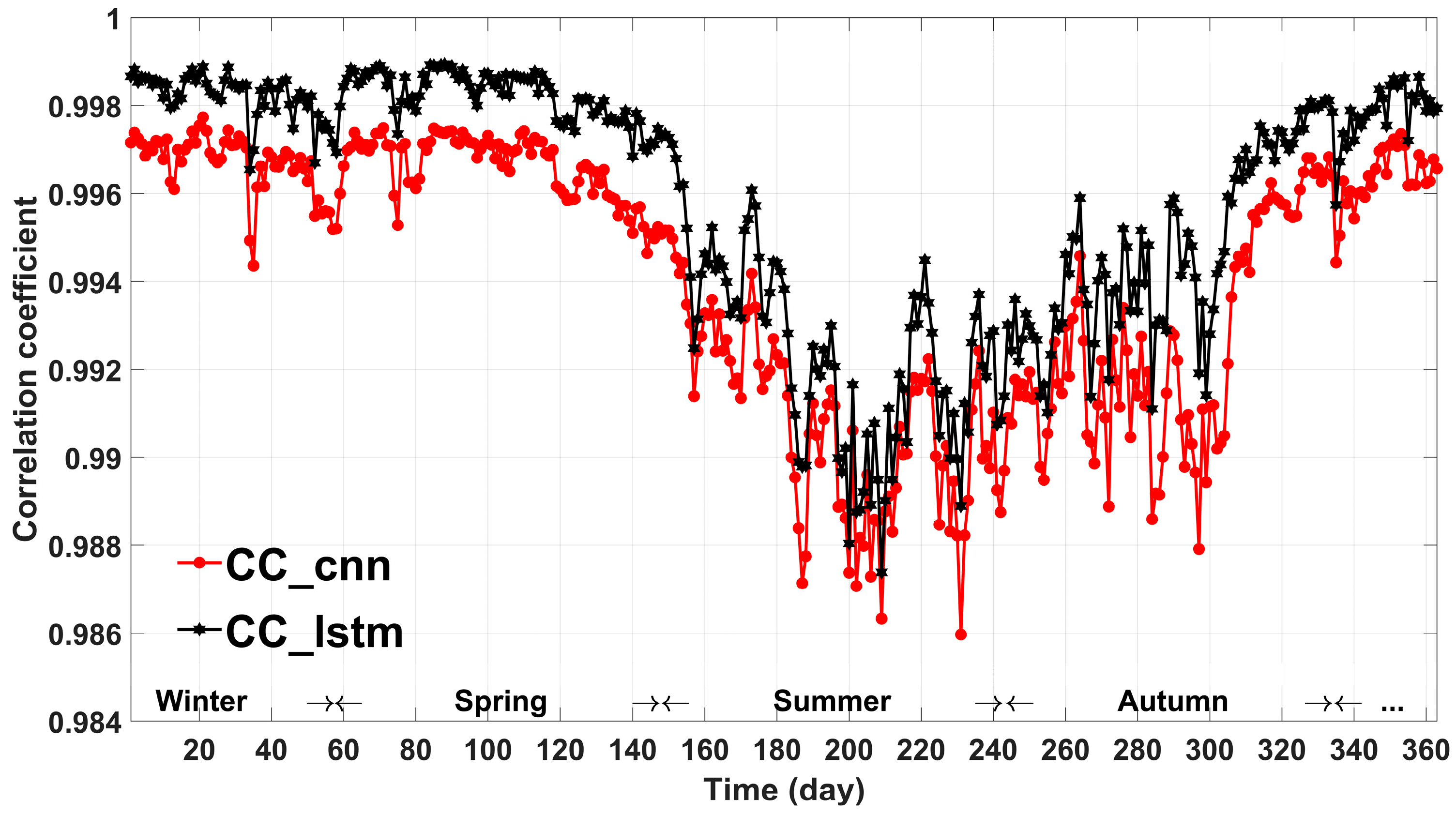
• In the 2018 test data, the SSIM of ConvLSTM always exceeded that of the CNNs (Figure 6). The highest SSIM of ConvLSTM was 0.977, the lowest was 0.874, while the highest SSIM of the CNNs was 0.957, and the lowest was 0.860. The CC of ConvLSTM was always higher than that of the CNNs (Figure 7). The highest CC of ConvLSTM was 0.999, the lowest was 0.987, while the highest SSIM of the CNNs was 0.997, and the lowest was 0.986. The spatial structure similarity and correlation of ConvLSTM for the tested 363 days were also higher than those of the CNNs.
• Taking the prediction results on 15 December as an example. Across the study area, the anomalies of ConvLSTM and CNNs were lower than the monthly average results (Figure 8). The anomality of the CNNs was higher than that of ConvLSTM, and that of the whole northeast channel was between −10% and 10%. The anomality of ConvLSTM was the lowest among the three methods, and the overall anomaly was between −5% and 5%. According to the comparison result, the monthly average result could not be used to replace the daily prediction of SIC.
• The RMSEs of the CNNs and ConvLSTM for the tested 363 days are compared in Figure 10. The RMSE of ConvLSTM was always lower than that of the CNNs. The highest RMSE of ConvLSTM is was 12.235%, and the lowest was 4.174%; the highest RMSE of the CNNs was 13.134%, and the lowest was 5.547%. The spatial distribution map of the RMSE in the Northeast Passage also showed that the monthly average results were the worst among the three, and ConvLSTM had the best prediction accuracy, particularly in the vicinity of the East Siberia Sea area.
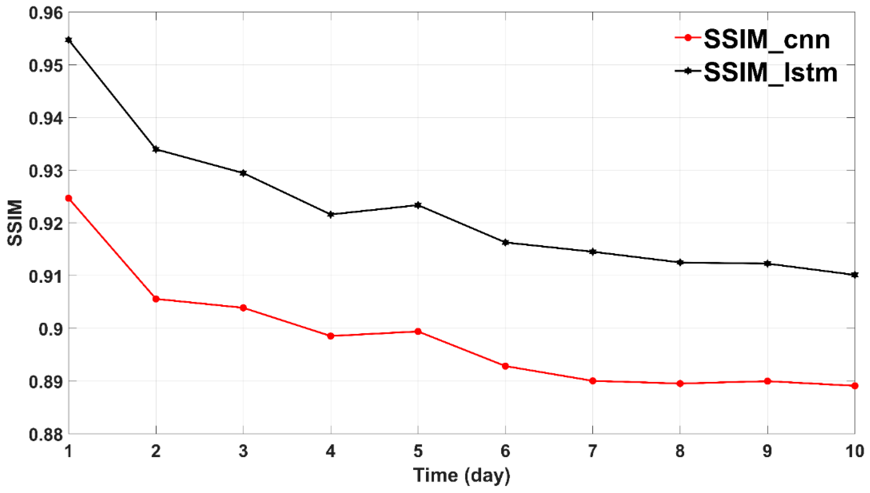
• In this study, the predictability of the CNNs and ConvLSTM was compared, and the SSIM and RMSE of the two were calculated through ten consecutive days of iterative prediction (Figure 13 and Figure 14). The average SSIM of the CNNs in these 10 d was 0.898, and the RMSE was 13.799%, while the average SSIM of ConvLSTM was 0.923, and the RMSE was 11.238%. According to the comparison results, the predictability of ConvLSTM was significantly better than that of the CNNs.

We proposed a 1-d SIC prediction model based on ConvLSTM. The daily SIC prediction results of ConvLSTM can provide valuable information that can be used in various decision-making processes, such as arctic track planning [5]. In addition, ConvLSTM may be applied to the daily prediction of sea ice thickness and other elements in future work.

References

1. Guemas, V.; Blanchard-Wrigglesworth, E.; Chevallier, M.; Day, J.J.; Déqué, M.; Doblas-Reyes, F.J.; Fučkar, N.S.; Germe, A.; Hawkins, E.; Keeley, S. A review on Arctic sea-ice predictability and prediction on seasonal to decadal time-scales. Q. J. R. Meteorol. Soc. 2016, 142. [Google Scholar] [CrossRef]
2. Screen, J.A.; Simmonds, I. The central role of diminishing sea ice in recent Arctic temperature amplification. Nature 2010, 464, 1334–1337. [Google Scholar] [CrossRef] [Green Version]
3. Francis, J.A.; Vavrus, S.J. Evidence for a wavier jet stream in response to rapid Arctic warming. Environ. Res. Lett. 2015. [Google Scholar] [CrossRef]
4. Stroeve, J.C.; Serreze, M.C.; Holland, M.M.; Kay, J.E.; Malanik, J.; Barrett, A.P. The Arctic’s rapidly shrinking sea ice cover: A research synthesis. Clim. Chang. 2012, 110, 1005–1027. [Google Scholar] [CrossRef] [Green Version]
5. Similä, M.; Lensu, M. Estimating the speed of ice-going ships by integrating SAR imagery and ship data from an automatic identification system. Remote Sens. 2018, 10, 1132. [Google Scholar] [CrossRef] [Green Version]
6. Hunke, E.C.; Lipscomb, W.H.; Turner, A.K.; Jeffery, N.; Elliott, S. CICE: The Los Alamos Sea Ice Model Documentation and Software User’s Manual Version 4.0 LA-CC-06-012; Los Alamos National Laboratory: Los Alamos, NM, USA, 2013; pp. 1–72.
7. Vancoppenolle, M.; Fichefet, T.; Goosse, H.; Bouillon, S.; Madec, G.; Maqueda, M.A.M. Simulating the mass balance and salinity of Arctic and Antarctic sea ice. 1. Model description and validation. Ocean Model. 2009, 27, 33–53. [Google Scholar] [CrossRef]
8. Hunke, E.C.; Lipscomb, W.H.; Turner, A.K. Sea-ice models for climate study: Retrospective and new directions. J. Glaciol. 2011, 56, 1162–1172. [Google Scholar] [CrossRef] [Green Version]
9. Girard, L.; Weiss, J.; Molines, J.M.; Barnier, B.; Bouillon, S. Evaluation of high-resolution sea ice models on the basis of statistical and scaling properties of Arctic sea ice drift and deformation. J. Geophys. Res. Ocean. 2009. [Google Scholar] [CrossRef]
10. Hutchings, J.K.; Roberts, A.; Geiger, C.A.; Richter-Menge, J. Spatial and temporal characterization of sea-ice deformation. Ann. Glaciol. 2011. [Google Scholar] [CrossRef] [Green Version]
11. Mudryk, L.R.; Derksen, C.; Howell, S.; Laliberté, F.; Thackeray, C.; Sospedra-Alfonso, R.; Vionnet, V.; Kushner, P.J.; Brown, R. Canadian snow and sea ice: Historical trends and projections. Cryosphere 2018, 12, 1157–1176. [Google Scholar] [CrossRef] [Green Version]
12. Lee, H.J.; Kwon, M.O.; Yeh, S.W.; Kwon, Y.O.; Park, W.; Park, J.H.; Kim, Y.H.; Alexander, M.A. Impact of poleward moisture transport from the North Pacific on the acceleration of sea ice loss in the Arctic since 2002. J. Clim. 2017, 30, 6757–6769. [Google Scholar] [CrossRef]
13. Smedsrud, L.H.; Halvorsen, M.H.; Stroeve, J.C.; Zhang, R.; Kloster, K. Fram Strait sea ice export variability and September Arctic sea ice extent over the last 80 years. Cryosphere 2017, 11, 65–79. [Google Scholar] [CrossRef] [Green Version]
14. Cox, C.J.; Uttal, T.; Long, C.N.; Stone, R.S.; Shupe, M.D.; Starkweather, S. The role of springtime arctic clouds in determining autumn sea ice extent. J. Clim. 2016, 29, 6581–6596. [Google Scholar] [CrossRef]
15. Carmack, E.; Polyakov, I.; Padman, L.; Fer, I.; Hunke, E.; Hutchings, J.; Jackson, J.; Kelley, D.; Kwok, R.; Layton, C.; et al. Toward quantifying the increasing role of oceanic heat in sea ice loss in the new arctic. Bull. Am. Meteorol. Soc. 2015, 96, 2079–2105. [Google Scholar] [CrossRef]
16. Wang, L.; Yuan, X.; Ting, M.; Li, C. Predicting summer arctic sea ice concentration intraseasonal variability using a vector autoregressive model. J. Clim. 2016, 29, 1529–1543. [Google Scholar] [CrossRef] [Green Version]
17. Wang, L.; Yuan, X.; Li, C. Subseasonal forecast of Arctic sea ice concentration via statistical approaches. Clim. Dyn. 2019, 52, 4953–4971. [Google Scholar] [CrossRef] [Green Version]
18. Chi, J.; Kim, H.C. Prediction of Arctic sea ice concentration using a fully data driven deep neural network. Remote Sens. 2017, 9, 1305. [Google Scholar] [CrossRef] [Green Version]
19. Kim, J.; Kim, K.; Cho, J.; Kang, Y.Q.; Yoon, H.J.; Lee, Y.W. Satellite-based prediction of arctic sea ice concentration using a deep neural network with multi-model ensemble. Remote Sens. 2019, 11, 19. [Google Scholar] [CrossRef] [Green Version]
20. Choi, M.; De Silva, L.W.A.; Yamaguchi, H. Artificial neural network for the short-term prediction of arctic sea ice concentration. Remote Sens. 2019, 11, 1071. [Google Scholar] [CrossRef] [Green Version]
21. Wang, L.; Scott, K.A.; Clausi, D.A. Sea ice concentration estimation during freeze-up from SAR imagery using a convolutional neural network. Remote Sens. 2017, 9, 408. [Google Scholar] [CrossRef]
22. Jun Kim, Y.; Kim, H.C.; Han, D.; Lee, S.; Im, J. Prediction of monthly Arctic sea ice concentrations using satellite and reanalysis data based on convolutional neural networks. Cryosphere 2020, 14, 1083–1104. [Google Scholar] [CrossRef] [Green Version]
23. Choi, K.S.; Nam, J.H.; Park, Y.J.; Ha, J.S.; Jeong, S.-Y. Northern sea route transit analysis for large cargo vessels. In Proceedings of the 25th International Symposium on Okhotsk Sea & Sea Ice, Mombetsu, Hokkaido, Japan, 21–26 February 2010; pp. 194–200. [Google Scholar]
24. Tschudi, M.A.; Meier, W.N.; Scott Stewart, J. An enhancement to sea ice motion and age products at the National Snow and Ice Data Center (NSIDC). Cryosphere 2020, 14, 1519–1536. [Google Scholar] [CrossRef]
25. Peng, G.; Meier, W.N.; Scott, D.J.; Savoie, M.H. A long-term and reproducible passive microwave sea ice concentration data record for climate studies and monitoring. Earth Syst. Sci. Data 2013, 5, 311–318. [Google Scholar] [CrossRef] [Green Version]
26. Cavalieri, D.J.; Gloersen, P.; Campbell, W.J. Determination of sea ice parameters with the NIMBUS 7 SMMR. J. Geophys. Res. Atmos. 1984, 89, 5355–5369. [Google Scholar] [CrossRef]
27. Comiso, J.C. Characteristics of Arctic winter sea ice from satellite multispectral microwave observations. J. Geophys. Res. Ocean. 1986, 91. [Google Scholar] [CrossRef]
28. Comiso, J.C.; Cavalieri, D.J.; Parkinson, C.L.; Gloersen, P. Passive Microwave Algorithms for Sea Ice Concentration: A Comparison of Two Techniques. Remote Sens. Environ. 1997, 60, 357–384. [Google Scholar] [CrossRef]
29. Kwok, R. Sea ice concentration estimates from satellite passive microwave radiometry and openings from SAR ice motion. Geophys. Res. Lett. 2002, 29, 24–25. [Google Scholar] [CrossRef]
30. Meier, W.N.; Peng, G.; Scott, D.J.; Savoie, M.H. Verification of a new NOAA/NSIDC passive microwave sea-ice concentration climate record. Polar Res. 2014, 33. [Google Scholar] [CrossRef] [Green Version]
31. Cavalieri, D.J. NASA Sea Ice Varidation Program for the DMSP SSM/I: Final Report. Nasa Tech. Memo. 1992, 96, 21969–21970. [Google Scholar]
32. LeCun, Y.; Bottou, L.; Bengio, Y.; Haffner, P. Gradient-based learning applied to document recognition. Proc. IEEE 1998, 86, 2278–2323. [Google Scholar] [CrossRef] [Green Version]
33. Yoo, C.; Han, D.; Im, J.; Bechtel, B. Comparison between convolutional neural networks and random forest for local climate zone classification in mega urban areas using Landsat images. ISPRS J. Photogramm. Remote Sens. 2019, 157, 155–170. [Google Scholar] [CrossRef]
34. Ren, S.; He, K.; Girshick, R.; Sun, J. Faster R-CNN: Towards Real-Time Object Detection with Region Proposal Networks. IEEE Trans. Pattern Anal. Mach. Intell. 2017, 39, 1137–1149. [Google Scholar] [CrossRef] [PubMed] [Green Version]
35. Zhang, Q.; Zhang, M.; Chen, T.; Sun, Z.; Ma, Y.; Yu, B. Recent advances in convolutional neural network acceleration. Neurocomputing 2019, 323, 37–51. [Google Scholar] [CrossRef] [Green Version]
36. Wang, R.; Luo, H.; Wang, Q.; Li, Z.; Zhao, F.; Huang, J. A Spatial-Temporal Positioning Algorithm Using Residual Network and LSTM. IEEE Trans. Instrum. Meas. 2020, 69, 9251–9261. [Google Scholar] [CrossRef]
37. Hochreiter, S.; Schmidhuber, J. LSTM Can Solve Hard Long Time Lag Problems. In Proceedings of the 9th International Conference on Neural Information Processing Systems; MIT Press: Cambridge, MA, USA, 1996; pp. 473–479. [Google Scholar]
38. Hu, W.S.; Li, H.C.; Pan, L.; Li, W.; Tao, R.; Du, Q. Spatial-Spectral Feature Extraction via Deep ConvLSTM Neural Networks for Hyperspectral Image Classification. IEEE Trans. Geosci. Remote Sens. 2020, 58, 4237–4250. [Google Scholar] [CrossRef]
39. Shi, X.; Chen, Z.; Wang, H.; Yeung, D.Y.; Wong, W.K.; Woo, W.C. Convolutional LSTM network: A machine learning approach for precipitation nowcasting. Adv. Neural Inf. Process. Syst. 2015, 2015-Janua, 802–810. [Google Scholar]
40. Abadi, M.; Paul, B.; Jianmin, C.; Zhifeng, C.; Andy, D.; Jeffrey, D. TensorFlow: A system for large-scale machine learning. Methods Enzymol. 1983, 101, 582–598. [Google Scholar] [CrossRef]
41. Kingma, D.P.; Ba, J. Adam: A Method for Stochastic Optimization. In Proceedings of the Contribution to International Conference on Learning Representations, San Diego, CA, USA, 7–9 May 2015. [Google Scholar]
42. Perovich, D.K.; Nghiem, S.V.; Markus, T.; Schweiger, A. Seasonal evolution and interannual variability of the local solar energy absorbed by the Arctic sea ice-ocean system. J. Geophys. Res. Ocean. 2007, 112, 1–13. [Google Scholar] [CrossRef]
43. Cavalieri, D.J.; Burns, B.A.; Onstott, R.G. Investigation of the effects of summer melt on the calculation of sea ice concentration using active and passive microwave data. J. Geophys. Res. 1990, 95, 5359–5369. [Google Scholar] [CrossRef]
44. Eicken, H.; Grenfell, T.C.; Perovich, D.K.; Richter-Menge, J.A.; Frey, K. Hydraulic controls of summer Arctic pack ice albedo. J. Geophys. Res. C Ocean. 2004, 109. [Google Scholar] [CrossRef] [Green Version]
45. Mäkynen, M.; Kern, S.; Rösel, A.; Pedersen, L.T. On the estimation of melt pond fraction on the arctic sea ice with ENVISAT WSM images. IEEE Trans. Geosci. Remote Sens. 2014, 52, 7366–7379. [Google Scholar] [CrossRef]
46. Kunkel, C. Essen im laufe der jahreszeiten: Der herbst. Akupunkt. und Tradit. Chinesische Medizin 2004, 32, 155–156. [Google Scholar]
47. Koenig, S.; Likhachev, M. Fast replanning for navigation in unknown terrain. IEEE Trans. Robot. 2005. [Google Scholar] [CrossRef]
48. Wang, Y.; Gao, Z.; Long, M.; Wang, J.; Yu, P.S. PredRNN++: Towards a resolution of the deep-in-time dilemma in spatiotemporal predictive learning. In Proceedings of the 35th International Conference on Machine Learning, Stockholm, Sweden, 10–15 July 2018. [Google Scholar]
49. Lee, S.; Stroeve, J.; Tsamados, M.; Khan, A.L. Machine learning approaches to retrieve pan-Arctic melt ponds from visible satellite imagery. Remote Sens. Environ. 2020, 247, 111919. [Google Scholar] [CrossRef]
50. Miao, X.; Xie, H.; Ackley, S.F.; Perovich, D.K.; Ke, C. Object-based detection of Arctic sea ice and melt ponds using high spatial resolution aerial photographs. Cold Reg. Sci. Technol. 2015, 119, 211–222. [Google Scholar] [CrossRef]
51. Knig, M.; Oppelt, N. A linear model to derive melt pond depth on Arctic sea ice from hyperspectral data. Cryosphere 2020, 14, 2567–2579. [Google Scholar] [CrossRef]
52. Popovi, P.; Silber, M.C.; Abbot, D.S. Critical Percolation Threshold Restricts Late-Summer Arctic Sea Ice Melt Pond Coverage. J. Geophys. Res. Ocean. 2020, 125. [Google Scholar] [CrossRef]
53. Li, Q.; Zhou, C.; Zheng, L.; Liu, T.; Yang, X. Monitoring evolution of melt ponds on first-year and multiyear sea ice in the Canadian Arctic Archipelago with optical satellite data. Ann. Glaciol. 2020, 61, 1–10. [Google Scholar] [CrossRef]
Figure 1. Schematic diagram of the sea area of the Northeast Passage (15 December 2018). Gray represents land, blue represents open water, and white represents sea ice.
Jmse 09 00330 g001
Figure 2. Model construction and comparison. SSIM refers to the structural similarity, and CC refers to the correlation coefficient.
Jmse 09 00330 g002
Figure 3. Schematic diagram of convolutional neural networks (CNNs) network structure. The yellow square represents the convolution kernel, and the gray square represents the feature map extracted by the convolution kernel.
Jmse 09 00330 g003
Figure 4. Convolutional long short-term memory network (ConvLSTM) network structure diagram. The meanings of each color in this figure are the same as those in Figure 3.
Jmse 09 00330 g004
Figure 5. Model and research flow.
Jmse 09 00330 g005
Figure 6. SSIM comparison of CNNs and ConvLSTM. The black line in the figure represents the SSIM of ConvLSTM, and the red line represents the SSIM of CNNs.
Jmse 09 00330 g006
Figure 7. Comparison of the CC of the CNNs and ConvLSTM. The black line in the figure represents the CC of ConvLSTM, and the red line represents the CC of CNNs.
Jmse 09 00330 g007
Figure 8. Comparison of the anomalies between different results, namely, monthly average (a), CNNs daily prediction (b), and ConvLSTM daily prediction (c) w.r.t the National Snow and Ice Data Centre (NSIDC) sea ice concentration (SIC) on 15 December 2018. The gray in the figure represents the land, and the blue/red represent the underestimation/overestimation of SIC. The area marked by the blue dotted line is the key contrast area in the following.
Jmse 09 00330 g008
Figure 9. Comparison of the anomalies between different results, namely, monthly average (a), CNNs daily prediction (b), and ConvLSTM daily prediction (c) w.r.t the NSIDC SIC near the Eastern Siberia sea area. The meanings of each color in this figure are the same as those in Figure 8.
Jmse 09 00330 g009
Figure 10. Comparison of the daily root-mean-squared-error (RMSE) between the CNNs and ConvLSTM. The magenta line in the figure represents the RMSE of ConvLSTM, and the blue line represents the RMSE of CNNs.
Jmse 09 00330 g010
Figure 11. Comparison of the monthly average (a), CNNs (b), and ConvLSTM (c) RMSEs of the Northeast Passage during December. The gray in the figure represents the land, and the red represents the RMSE of each model in December. The area marked by the blue dotted line is the key contrast area in the following.
Jmse 09 00330 g011
Figure 12. Comparison of the RMSE between the monthly average (a), CNNs (b) and ConvLSTM (c) data near the Eastern Siberian sea area. The meanings of each color in this figure are the same as those in Figure 11.
Jmse 09 00330 g012
Figure 13. Comparison of the SSIM between the iterative prediction by the CNNs and ConvLSTM. The black and red lines represent the SSIM of ConvLSTM and CNNs, respectively.
Jmse 09 00330 g013
Figure 14. Comparison of the RMSEs of the iterative prediction by the CNNs and ConvLSTM. The magenta and blue lines represent the RMSE of ConvLSTM and CNNs, respectively.
Jmse 09 00330 g014