
Simulating the Coastal Ocean Circulation Near the Cape Peninsula Using a Coupled Numerical Model


1
Marine Research Unit, South African Weather Service, Cape Town 7525, South Africa
2
Department of Oceanography, University of Cape Town, Rondebosch 7701, South Africa
3
National Sea Rescue Institute, Cape Town 8005, South Africa
4
Marine and Antarctic Research centre for Innovation and Sustainability (MARIS), University of Cape Town, Rondebosch 7701, South Africa
5
Coastal and Estuarine Processes, National Institute for Water and Atmospheric Research, Hamilton 3216, New Zealand
6
Institute for Coastal and Marine Research, Nelson Mandela University, Port Elizabeth 6031, South Africa
*
Author to whom correspondence should be addressed.
J. Mar. Sci. Eng. 2021, 9(4), 359; https://0-doi-org.brum.beds.ac.uk/10.3390/jmse9040359
Submission received: 12 February 2021
/
Revised: 9 March 2021
/
Accepted: 15 March 2021
/
Published: 26 March 2021
(This article belongs to the Special Issue Monitoring and Modelling of Coastal Environment)
Abstract
:A coupled numerical hydrodynamic model is presented for the Cape Peninsula region of South Africa. The model is intended to support a range of interdisciplinary coastal management and research applications, given the multifaceted socio-economic and ecological value of the study area. Calibration and validation are presented, with the model reproducing the mean circulation well. Maximum differences between modelled and measured mean surface current speeds and directions of 3.9 × 10⁻² m s−1 and 20.7°, respectively, were produced near Cape Town, where current velocities are moderate. At other measurement sites, the model closely reproduces mean surface and near-bed current speeds and directions and outperforms a global model. In simulating sub-daily velocity variability, the model’s skill is moderate, and similar to that of a global model, where comparison is possible. It offers the distinct advantage of producing information where the global model cannot, however. Validation for temperature and salinity is provided, indicating promising performance. The model produces a range of expected dynamical features for the domain including upwelling and vertical current shear. Nuances in circulation patterns are revealed; specifically, the development of rotational flow patterns within False Bay is qualified and an eddy in Table Bay is identified.
1. Introduction
1.1. Geographical Context
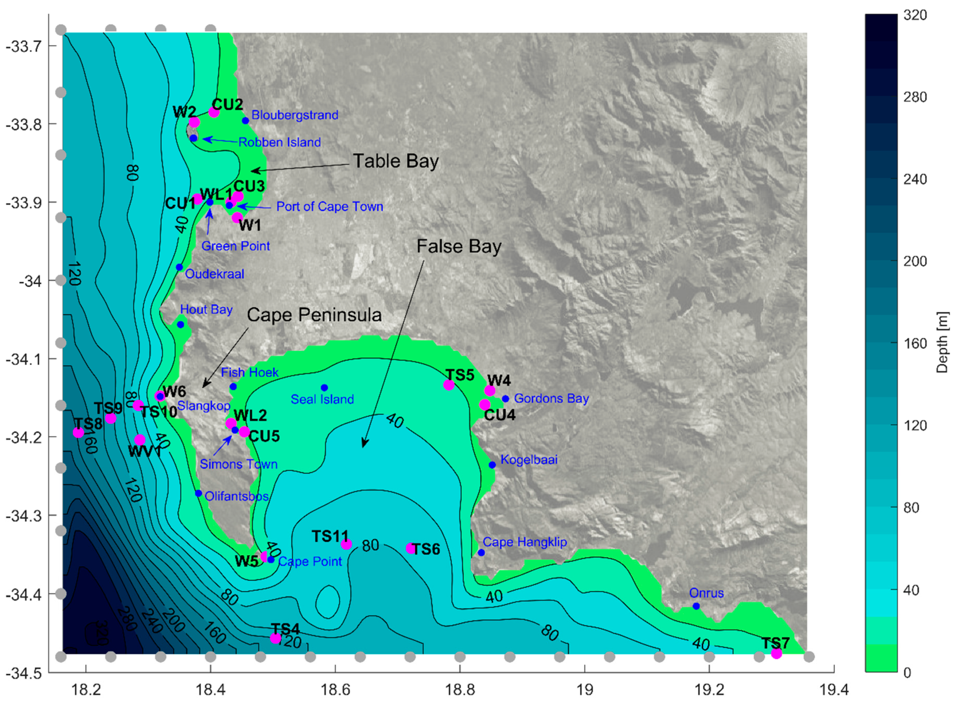
The Cape Peninsula area, situated along the southwest coast of South Africa, is defined by Table Bay to the north and False Bay to the south (Figure 1). These bays exhibit complex meteorological-oceanographic dynamics as a result of, among other factors, complex orography, bathymetry [1] and coastal orientation, and the meeting and mixing of warm Agulhas Current waters and cold Benguela currents [2,3,4].
Table Bay is a relatively small, shallow embayment [5], reaching a depth maximum of around 35 m and covering an area of approximately 100 km2 [6]. Considering the Bay as existing between the two headlands at Bloubergstrand and Green Point [6], the mouth of the Bay is predominantly north-west and west facing. The famous Robben Island is located to the northwest of the Bay. Immediately west of the Port of Cape Town, a rocky coastline extends southwards until Cape Point, forming the western shoreline of the Cape Peninsula.
False Bay is a southward facing embayment defined by Cape Point (the southern point of the Cape Peninsula) in the west and Cape Hangklip in the east. It is the largest bay in South Africa, covering an area of approximately 1000 km2 [7] and is roughly rectangular, making it relatively unique globally [8]. False Bay’s coastline is dynamic, with rugged, rocky shores and nearby mountains in the west and east, and transient sandy beaches in the north [2,7]. Depths increase gradually towards the mouth of the Bay, reaching between 80 and 100 m across the southern boundary [2,7,8,9]. Notably, several rocky pinnacles and steep-sided reefs are dotted throughout the Bay [2], breaking otherwise gradually offshore-sloping bathymetry.
The study domain hosts a multitude of social (e.g., [10]), economic [10,11] and ecological [12] interests. It supports thriving tourism [13,14], recreation [7,13], fishing [7,15] and shipping [16] activities of various scales and types. The complex interactions between these dimensions, against a backdrop of dynamic, storm prone environmental forcing and climate change, make robust coastal management important [11,17].
1.2. Synoptic Weather Influences
The study domain is dominated by two principal synoptic meteorological regimes arising from its latitudinal position. In summer, the south-Atlantic anticyclone is situated west of southern Africa, giving rise to frequent, strong south-easterly winds over Cape Town. In winter, the south-Atlantic anticyclone migrates northwards, allowing transient midlatitude cyclones and coastal low pressures to brush the domain, bringing north-westerly and westerly winds following the passing of low-pressure systems and ahead of cold fronts. These north-westerly and westerly winds dominate during colder months, though to a lesser extent than the south-easterly winds during summer, which occur even during colder months [18,19,20]. After a cold front has passed, south-westerly winds are possible as a high-pressure system ridges towards the study domain [20].
1.3. Existing Knowledge of the Circulation
In the early nineties, Ref. [6] highlighted the deficiency of information on the physical oceanography of Table Bay. That which was available was generally dispersed and inaccessible, consisting mostly of commercial reports. The situation remains largely unchanged today. The status of information for False Bay is similar, with Ref. [7] noting that direct observations of the circulation in False Bay are scarce and old. While several studies from the 1970 and 1980s investigated the circulation of False Bay [21], a coherent overview of the circulation remains lacking owing to the spatio-temporal fragmentation of sampling [22]. A brief summary of salient findings for Table Bay, the Western Peninsula and False Bay follows.
1.3.1. Table Bay
Currents are generally weak and variable throughout the water column, with bottom currents weaker than surface currents and often almost stagnant [5,6]. The circulation is overwhelmingly wind-driven [5,6]; a characteristic augmented by the shallowness of the Bay and negligible influence of remote forcing or far-field currents [5,23,24]. The two prevailing wind directions in Table Bay have been observed to drive a bimodal circulation regime. South-easterly winds impart an anti-clockwise circulation, with water transport focused generally northwards (bearings 270°–090° true). North-westerly winds impart a clockwise circulation, with water transport focused generally southwards (bearings 090°–270° true) [5]. Tides are of secondary forcing importance to winds. Given a modest tidal range around 1.8 m at spring maximum [5,25], the currents they drive are weak [5]. In the nearshore, surface gravity waves are the dominant forcing driving currents [5,6,23]. This mechanism was explained for a small embayment just north of the study site by Refs. [26,27] and applies to prevailing south-westerly waves striking the coastline along the eastern margins of Table Bay obliquely, thereby establishing a dominant northward current close to the shore [5,23].
Salinities were fairly homogenous throughout the Bay, ranging between 34.4 and 35.5, but mostly between 34.7 and 35.3 [5]. Sea temperatures in Table Bay appear to be strongly influenced by nearby wind-driven upwelling centres; specifically Cape Columbine to the north, and Oudekraal and Slangkop just a few kilometers to the south [4,6,28]. From August-October (the simulation period for this study) mean SSTs of 13–14 °C can be expected in Table Bay [28].
1.3.2. Western Peninsula
The region stretching from Cape Point northwards towards Table Bay connects the two embayments of interest. Between Cape Point and Slangkop, currents are well correlated with winds. Ref. [9] observed that south easterly (north-westerly) winds during summer (winter) drive predominantly northward (southward) flow along this coastline. This agrees with Ref. [4], who noted strong current reversals off Olifantsbos from northward to southward when winds went from southerly to northerly and vice versa, and Ref. [29], who also emphasized the importance of local wind-generated currents in this region. Between Slangkop and Table Bay, currents become very complex close to the coast. An investigation of the circulation at Camps Bay revealed little circulatory correlation with local winds [9,30]. Near Green Point, a wind shadow created by the nearby mountains, shields this area from frequent south-easterly winds. Slightly further offshore (perhaps beyond the wind shadow), summer flow has been shown to be between 60° and 120° true around 70% of the time [9,31]. In winter, currents are more directionally variable with 36% of currents being between northerly and westerly, and around 54% being between westerly and southerly.
The upwelling centres mentioned previously are located along this stretch, near Oudekraal and Slangkop, with semi-permanent upwelling occurring in response to south-easterly winds. Resulting plumes of upwelled water are directed offshore and west of Robben Island [9,32]. Downwelling was observed during north-westerly winds along the Peninsula [4,32] though it appeared confined to the upper 50 m [4].
Density along the western Peninsula is strongly temperature-controlled, with isopycnals adhering closely to isotherms both vertically and horizontally [4].
1.3.3. False Bay
Four main surface circulation patterns have been observed in False Bay, being first observed by Ref. [33]. Wind forcing (responsible for the first two patterns described below) is clearly dominant in False Bay with tidal and inertial currents being of secondary importance, particularly during times of weak winds [8,21,33,34,35].
The first of these is a clockwise rotation, observed mostly during summer and driven by the frequent south-easterly winds. This pattern was further observed by Ref. [35], and modelled by Ref. [22]. The circulation within the Bay under these conditions is partially set up by west-north-westerly flow south of the Bay splitting at Cape Point, with the northerly arm then establishing equatorward flow along the western shores [8,18,33]. The frequency of south-easterly winds results in this clockwise regime dominating [33,35]. Ref. [35] qualified this pattern by noting poleward motion at Cape Point, which prevented true cyclonic motion over the whole Bay. The second is an anti-clockwise rotation in response to north-westerly winds, with an eastwards current flowing south of the Bay entering at Cape Hangklip [9,33,35]. The third and fourth patterns arise from tidal forcing during outgoing and incoming tides respectively. They are permitted to develop in the absence of strong wind forcing [8,33], with fairly uniform northward flow during incoming tides, southward flow during outgoing tides, and bathymetric steering in shallow regions. Ref. [35] found tides to generate currents along the perimeter of the Bay and in the shallowing northern reaches between Simonstown and Gordon’s Bay. At the mouth of the Bay, tidal and inertial currents appeared to be regular contributors to the overall variability in the lower half of the water column (along with the familiar meteorological periodicity evident in the wind-driven variability) [8]. Energy from surface gravity waves and focused by bathymetry immediately outside and within the Bay are important drivers of currents in the nearshore, particularly in the northern reaches [35,36].
Density dynamics in the Bay are predominantly temperature controlled, with only weak contributions from salinity [37]. Temperature is affected by wind via upwelling and advection of cold water, with insolation playing a secondary role, especially in the northerly and north-easterly shallows [8,34,35,37]. Ref. [38], however, determined waves to control nearshore temperatures to a greater degree than wind. The most notable thermal feature is upwelling of cold water north-west of Hangklip, and to a lesser extent, Gordon’s Bay, in response to strong south-easterly winds [22,34,35,37]. Upwelling was also observed along the coastal stretch up to 20 km east of Hangklip, in turn supplying cold water to both Hangklip and the interior of the Bay [18,37]. The Bay is generally thermally stratified in summer, with a well-developed thermocline and relatively higher vertical temperature variability. It is generally well-mixed and uniformly colder in winter [8,18,34,35]. SSTs during the simulation period for this study (August-October) could be expected to range between 14.5 and 17 °C [34].
1.4. The Case for a Coastal Model
Owing to the importance of the study domain, rising stress due to increased coastal activity (e.g., [8,37,38,39]) and climate change, demand for routine measurements and forecasts of coastal ocean currents and other marine parameters is increasing [40,41]. This stems from the need to support various applications including, but not limited to, coastal management (encompassing recreation, fisheries, aquaculture, water quality, sewage spills/outfall, flooding, beach erosion and harmful algal bloom management), maritime navigation safety and efficiency, search and rescue and support to biogeophysical/biogeochemical [5,40,41,42,43]. It is thereby proposed that a coastal ocean modelling system is an important part of the science-for-management [44] component of an integrated coastal management framework for the Cape Peninsula area.
While several global ocean reanalysis, analysis and forecast models cover coastal domains in a broad sense, distinct systems are required to derive useful information for coastal domains. Many coastal parameters of interest, including tides, storm surges, currents, surface waves and bathymetry, are specific to coastal seas, and their representation absent in any practical sense from global models [40]. Related to this is the question of spatio-temporal resolution, which is generally far higher when making predictions of coastal conditions than those of the adjacent deep oceans. For example, sea level and current variability on shelves is often dominated by the effects of tides, internal wave breaking and high frequency atmospheric forcing, with time scales of hours and horizontal scales down to hundreds of meters or less being relevant [40].
By downscaling to smaller computational domains of higher spatial resolution, using boundary information from global models and higher resolution atmospheric forcing, and including relevant physical drivers, useful coastal ocean characterizations can be produced [40]. This one-way nesting approach has been successfully used in other coastal areas. Most recently, a configuration of Delft3D Flow [45,46] and SWAN [47] was implemented by [48], in a similar application to this study, to assess the influence of varying wind fields on forecasts of coastal dynamics near North Carolina, USA. Boundary and atmospheric forcing from various global models were used to provide appropriately downscaled wave, current and water level estimates. Ref. [49] used boundary conditions from a 12 km regional model for a series of one-way nested, downscaled domains in the California Current system, demonstrating a regime transition from mesoscale to sub-mesocale at scales < 1 km for a typical summer wind system. Ref. [41] applied a tiered one-way nesting approach to the Rio de la Plata coastal region near Argentina and Uruguay. Using a limited-area 5–9 km resolution parent domain, a series of 2 km, 1 km and 0.1 km nests was implemented to arrive at a resolution sufficient to support Lagrangian particle water quality modelling. Ref. [50] adopted a similar approach, with a limited area parent domain varying between 15 km offshore and 200–300 m nearer the coast, and an online-nested intermediate grid of around 100 m resolution. A highly refined (down to 25 m) model grid was then tested via one-way nesting in the intermediate and parent grids, with the intermediate grid performing similarly to the finest resolution offline nest, but the offline nest performing well only when run with boundary conditions from the intermediate model. This suggests that the resolution and definition of boundary conditions in coastal areas are potentially highly important, and that the full potential of the very high resolution might only be unlocked with similarly high-resolution bathymetry.
Such a system could be deployed for rapid tasking in response to oil spill events, specific coastal management or design questions or search and rescue cases, for example. The system could also provide operational predictions by applying suitable available boundary condition and forcing in forecast mode. In forecasting storm surge and waves, this approach has been successfully demonstrated by Ref. [51] using Delft3D Flow [45,46,52] and SWAN [47]. In forecast mode, model error can be further constrained by improving initialization via data assimilation. This has been successfully demonstrated in a similar application using the Delft3D Flow circulation model and OpenDA for data assimilation by Ref. [53].
This purpose of this study was to build and describe a hydrodynamical model to provide a basic characterisation of the circulation near the Cape Peninsula, and which could be further deployed to support interdisciplinary coastal applications.
2. Data and Methods
2.1. Numerical Models
The numerical model employed in this study is a coupled configuration of Delft3D Flow [45,46] and SWAN [47], providing hydrodynamic and wave simulations, respectively. The modelling system is built within the Delft3D environment and is referred to hereafter as the High-Resolution Model (HRM) to distinguish it from measurements and the Global Ocean Forecast System 3.1 [54], an implementation of version 2.2.99DH of the HYbrid Coordinate Ocean Model (HYCOM; [55]), which is also used in this study. Delft3D Flow has been extensively used in ocean and coastal domains [56] and the reliability of its code variously established [57,58,59]. The model has been successfully applied in cases similar to the one in this study (e.g., [48,50,53,60,61]).
Delft3D Flow is a three-dimensional circulation model which solves the unsteady Reynolds averaged Navier Stokes equations (RANS; [62]. For a comprehensive description of the system of equations employed by Delft 3D Flow, the reader is referred to Ref. [46]. SWAN is a third generation spectral wave model which has been successfully used in a range of coastal applications [47,63,64,65,66]. Furthermore, SWAN has been reliably implemented in the present study domain by Ref. [51] as part of a coupled wave and storm surge forecasting system.
The choice to couple a wave model to the circulation component provides various advantages. Future interdisciplinary applications of the model, such as trajectory modelling for search and rescue or pollution management, could benefit from wave information directly (e.g., wave height, period and direction), as well as from information on wave-induced Stokes drift, and modification of the Eulerian mean flow through wave–current interactions. These processes are important in the transfer of momentum and thereby the modelling of surface drift [67,68,69]. In Delft3D Flow, they are driven by wave-induced radiation stress from the coupled SWAN model and momentum transfer due to breaking waves, computed by a sub-model [70,71]. Furthermore, the literature ascribes importance to wave-driven currents in the study domain, especially in the nearshore (e.g., [5,24,26,27,35,36]), with the coupled approach having the potential to resolve such processes. Moreover, Ref. [38] determined a stronger dependency on waves than wind for nearshore SST within False Bay. By including the dominant local forcings of winds, tides, waves and atmospheric heat fluxes (e.g., [5,6,8,9,21,33,34,35]) and in coastal domains generally [40], and increasing resolution to harness the benefit of high atmospheric and bathymetric resolutions, it is asserted that the model accounts for the most important relevant processes. Furthermore, while an overarching focus of this preliminary effort is the simulation of surface phenomena due to their importance for search and rescue, hydrostatic models have been shown to reproduce sub-mesoscale ocean fronts and vertical structures at scales between 0.5 and 1 km successfully [72,73]. Wind forcing quality and grid resolution appear to be far more critical in this regard [72,73]. Being very short-lived, non-hydrostatic phenomena also account for just a small fraction of the energy in typical coastal oceans, with RANS turbulence closure schemes having been shown to represent unresolved non-hydrostatic processes reasonably well [74]. The inclusion of non-hydrostatic pressure terms for predictions at time scales longer than 1 h is unlikely to provide significant benefit [74].
2.1.1. Model Grid
Several considerations guided the selection of horizontal resolution for this first modelling effort. The features of interest (sub-bay scale) require higher resolution than that afforded by global or regional models. In this regard, a combination of the relevant processes and sufficient grid resolution to discriminate features within Table and False Bay is sought. At the very least, the resolution should guide future modelling or measurement work, by providing insight into the importance of various processes. Furthermore, future applications of the model requiring higher resolution to be effective, such as particle tracking within the embayments, were considered. It is acknowledged that there is a rigorous community effort underway to deliver operational ocean reanalyses and forecasts at resolutions typically between 1/10° and 1/12°. This study is intended to complement these efforts by translating their information (which is sparse in the coastal-nearshore context but crucial as boundary conditions) to the coastal domain with higher frequency and spatial detail. The HRM is discretized on a boundary-fitted orthogonal curvilinear grid, covering the area of interest as shown in Figure 1. The grid was designed to align with the global HYCOM grid from which boundary conditions and reference data were later extracted, with 12 cells per HYCOM cell. This was done to minimize spurious boundary effects in the communication of information from the coarser global model. The resulting horizontal resolution of the grid is 1/144° or 600–750 m across the domain. The model uses 10 sigma layers in the vertical with higher resolution near the surface and the bed. A computational time step of 0.75 s was selected to satisfy Courant-Friedrichs-Lewy (CFL) considerations, with model output produced with an hourly temporal resolution.
2.1.2. Bathymetry
Composite bathymetry was assembled by interpolating freely available 1′ General Bathymetric Chart of the Oceans (GEBCO) data with high-resolution soundings provided by the South African Navy Hydrographic Office (SANHO). The bathymetry is matched to the HYCOM bathymetry along open boundaries and smoothed three cells inwards. This facilitates smoother interpolation of vertical boundary conditions from one model to the next.
2.1.3. Open Boundary Conditions
Space-time varying temperature and salinity boundary conditions were prescribed in the horizontal and vertical at the HRM’s open boundaries and updated every 3 h. These data were extracted from the Global Ocean Forecasting System (GOFS) 3.1 Reanalysis product [54], produced by the United States Naval Research Laboratory: Ocean Dynamics and Prediction Branch (available: https://www.hycom.org/dataserver/gofs-3pt1/reanalysis, accessed on 26 June 2020). GOFS 3.1 has a horizontal resolution of 0.08°, or around 8.9 km, and 41 vertical layers, and is made available with 3-hourly temporal resolution. Hereafter, GOFS 3.1 will be referred to as “HYCOM”. Space-time varying astronomic water level boundary conditions, extracted from the TPXO 7.2 global inverse tide model [75] were also applied at the open circulation boundaries. TPXO 7.2 is currently widely used and was selected here having been robustly validated in for the South African region by [76]. Space-time varying parameter wave boundary conditions from the National Centers for Environmental Prediction (NCEP) operational forecasting model (WaveWatch III), with a resolution of 0.5°, are prescribed at the SWAN model’s open boundaries. A JONSWAP spectrum [77] is assumed, with constant peak enhancement factor of 2.5 following Ref. [78]. A constant wave directional spreading of 25° was also assumed following Ref. [51].
2.1.4. Atmospheric and Tidal Forcing
Space-time varying 10 m winds from the Wind Atlas of South Africa [79], which is a downscaling of the ERA-Interim (ERA-I) reanalysis product [80] using the Weather Research and Forecasting model [81], are applied to the wave and circulation models. The forcing has a horizontal resolution of 0.03°, or roughly 3 km and a 1-h temporal resolution. Hourly sea-level pressure data are applied to the coupled wave and circulation models in order that inverse barometric forcing on water levels is included. These space-time varying data are taken from the ERA-I product [82] for coherence with the wind forcing. ERA-I has a resolution of approximately 79 km but is also provided at a resolution of approximately 13.9 km (used here) via ECMWF’s bi-linear interpolation technique for continuous variables. Total cloud cover, 2 m air temperature and dew point temperature variables are also taken from ERA-I, the latter two from which relative humidity is computed. Two m air temperature, relative humidity and total cloud cover are then supplied to the HRM to force surface heat fluxes. Heat fluxes are computed by Delft3D’s Ocean heat flux model following Refs. [83,84]. The effect of Newtonian gravitational forces on the water mass within the HRM domain is accounted for via the most important semi-diurnal, diurnal and long period harmonic constituents (11 in total). While some very small-scale coastal models neglect this forcing, increasing domain size, deeper bathymetric regions and/or the modelling of enclosed basins require that these gravitational effects be accounted for [45].
2.2. HRM Calibration and Validation
Circulation model calibration and validation was conducted following the guidelines established by Ref. [85]. Model runs were conducted in an iterative fashion, with each configuration varying by a single parameterization setting in order to optimize that setting. Model performance was assessed according to the available measured data water level and current data by computing Root Mean Square Errors (RMSE). Bottom roughness, wind drag breakpoint coefficients, horizontal and vertical eddy viscosity, horizontal and vertical eddy diffusion, turbulence closure schemes, Dalton numbers and Stanton numbers (for heat fluxes) were tested. The HRM simulation is initialized from quiescent conditions and is allowed to spin up for two weeks prior to analysis, by which time the transient solution has died out.
Wave model calibration settings determined by [51] were applied, except for the white-capping parameterisation. This was set to the Van Der Westhuysen model for its ability to handle mixed sea/swell conditions and perform well in the nearshore [52].
2.2.1. Calibration Data
HRM performance in each calibration run was assessed by comparing results to available measured water level and current data. In the case of currents, velocity time series for two depth levels were assessed for the sake of practicality. Near-surface and near-bottom velocities were extracted from HRM layers 2 and 9 (of 10), respectively. Given the sigma vertical coordinate framework, the depth ranges of these layers vary slightly between sites, being 8% of the water depth. Measured velocities from the closest matching depths to the mean depths of these HRM layers were then used for comparison. HYCOM time series from the closest available grid cells were extracted in the same way, for reference. Hourly water level measurements for Cape Town and Simon’s Town were obtained from the South African Navy Hydrographic Office (SANHO) and vertical profile current measurements from an Acoustic Doppler Current Profiler (ADCP) for a point in the south-western reaches of Table Bay were obtained from the Transnet National Ports Authority (TNPA).
2.2.2. Validation Data
Meteorological forcing data were validated by comparison to available measurements from various automatic weather stations (AWS) around the model domain, namely Royal Cape Yacht Club (RCYC), Robben Island, Strand, Cape Point and Slangkop. Validation of the HRM was then performed in the same way as calibration, but for different points in space and time to those used during calibration, following [85]. Additionally, results are presented for temperature and salinity profiles obtained from the Word Ocean Database (WOD). A total of eight profiles over 4 days were available for the relevant time periods. Since the availability of relevant temperature and salinity data was very limited, they are not used for calibration. The snapshot profile comparisons provide cursory insight into the simulation of these parameters by the model. The wave component of the HRM was not re-calibrated in this study, with settings from Ref. [51] having been used. Available measurements of significant wave height (Hs), peak period (Tp) and peak direction (Dp) from the Datawell Waverider buoy off Slangkop could thus be used to present validation statistics for that location, having not been used in calibration (following Ref. [85]). Figure 1 provides a spatial overview of the model domains and various measurements used in calibration and validation.
3. Results and Discussion
3.1. Atmospheric Forcing Validation
Given the central importance of wind in driving coastal hydrodynamics both generally and specifically in this domain (e.g., [5,6,8,21,33,34,35]), the quality of atmospheric forcing (wind and pressure) was assessed. Wind speeds were adjusted to the 10 m reference level for fair comparison with the WASA forcing by means of the Log Law for wind profile correction [86], using a roughness length of 3.5 × 10⁻⁴ m (the mid-point value between those for calm, open seas and wind-blown oceans [87]). Computed RMSEs indicate reasonably good agreement with measurements (Table A1 in Appendix A). Some degree of error is inevitable given the relatively high, but nonetheless limiting, horizontal resolution of 3 km, which makes resolving the complex orography around the study domain challenging. Sea-level pressure (SLP) signals were reproduced faithfully, albeit that the ERA-I product exhibited a very slight positive bias in all cases (Figure S1). While the 10 m wind velocity signals were reasonably well simulated, there are times during which errors (particularly in direction) are noticeable (Figure S2). This is likely due to sub-grid scale effects such as sheltering and deflection due to mountains.
3.2. HRM Calibration Settings
The final set of calibration settings determined according to the process explained in Section 2.2 is given in Table 1.
3.3. HRM Calibration Performance
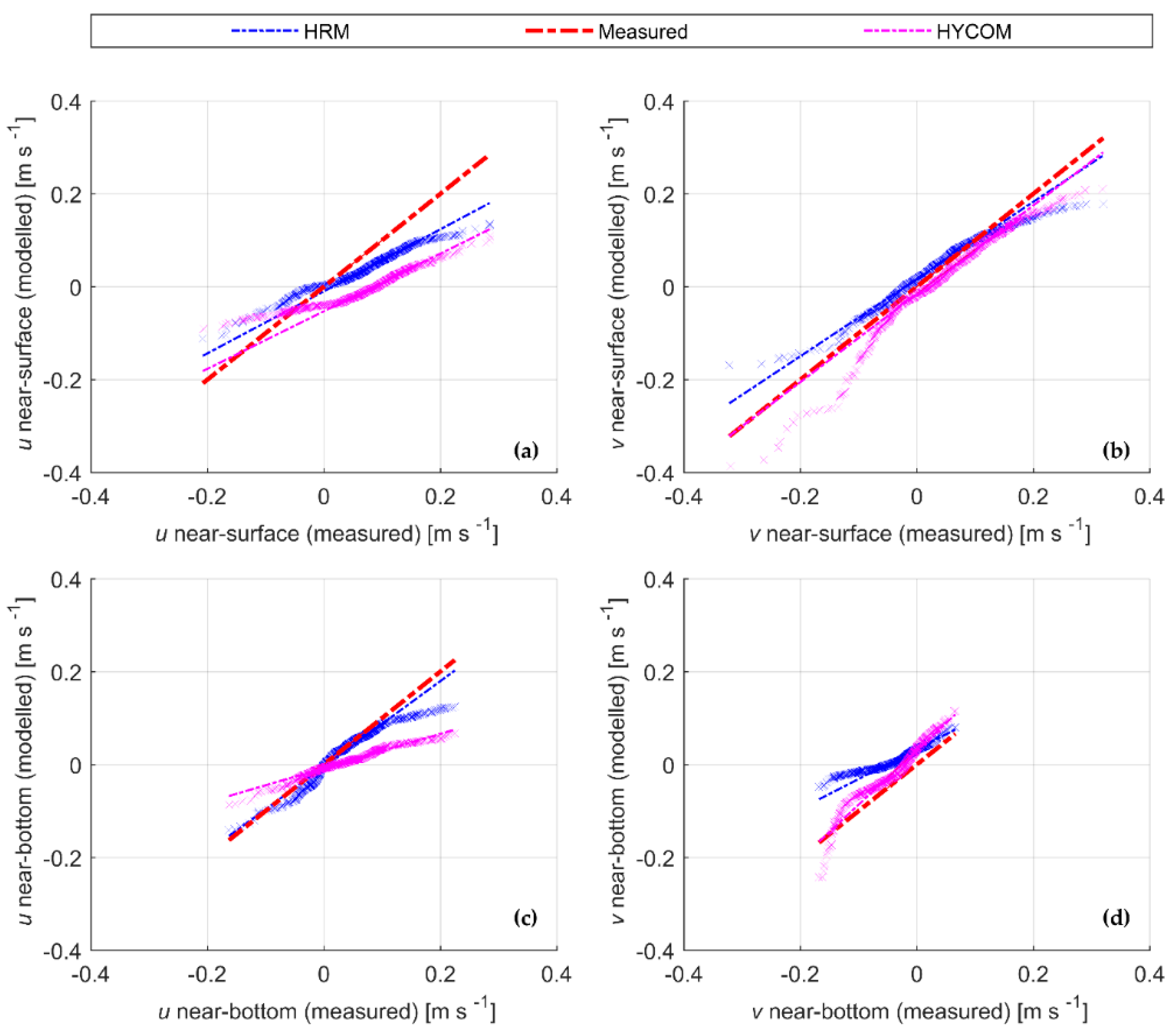
Calibration accuracies are presented in Table A2 in Appendix A. Systematic tuning of the model parameterisation settings resulted in water level calibration RMSE of 0.21 m and 0.10 m at Cape Town (Site WL1) and Simon’s Town (site WL2), respectively. Near Cape Town (site CU1), RMSE for near-surface and near-bottom velocity components ranges between 0.064 and 0.100 m s−1. Surface velocities show marginally higher absolute errors, but this is to be expected since absolute surface speeds are higher than those near the bed. These vector accuracies result in RMSEs for near surface (bottom) current speeds of 0.080 (0.065) m s−1 and average angular directional errors for near-surface (bottom) currents of 59.8 (69.1)° TN. The mean surface flow is reasonably well reproduced, with average near-surface current speeds and directions of 8.8 × 10⁻² m s−1 and 74.8° TN, compared to corresponding average speed and direction measurements of 12.8 × 10⁻² m s−1 and 96.5° TN respectively. Near the seabed, the mean modelled and measured speeds and directions were 5.8 and 7.7 × 10⁻² m s−1, and 121.9 and 145.1° TN, respectively. This represents an improvement over the global model for all except near-bottom current directions (refer to Table A3. Notwithstanding the reproduction of the mean flow, certain high-frequency fluctuations are not resolved by the HRM specifically where short-lived reversals or higher-speed flows occur. These specific inaccuracies at certain times contribute to increased RMSE. Moreover, velocities are weak and variable throughout. In the absence of strong flow signals, bathymetric and other model artefacts are of higher relative importance, making the accurate simulation of the flow more difficult.
Figure 2 shows quantile-quantile assessments of the modelled and measured velocity distributions at calibration site CU1. Corresponding time series plots are available in the supplementary material (Figures S3 and S4). In all cases except that of meridional near-bottom flows, the HRM velocity distributions adhere more closely to the measured distributions than the global model distributions. At the surface, zonal HRM velocities tend to be underestimated. Additionally, near the surface, higher meridional velocities are very slightly underestimated. Near-bottom zonal flows are very well reproduced by the HRM, but both the HRM and HYCOM both tend to underestimate southward velocities.
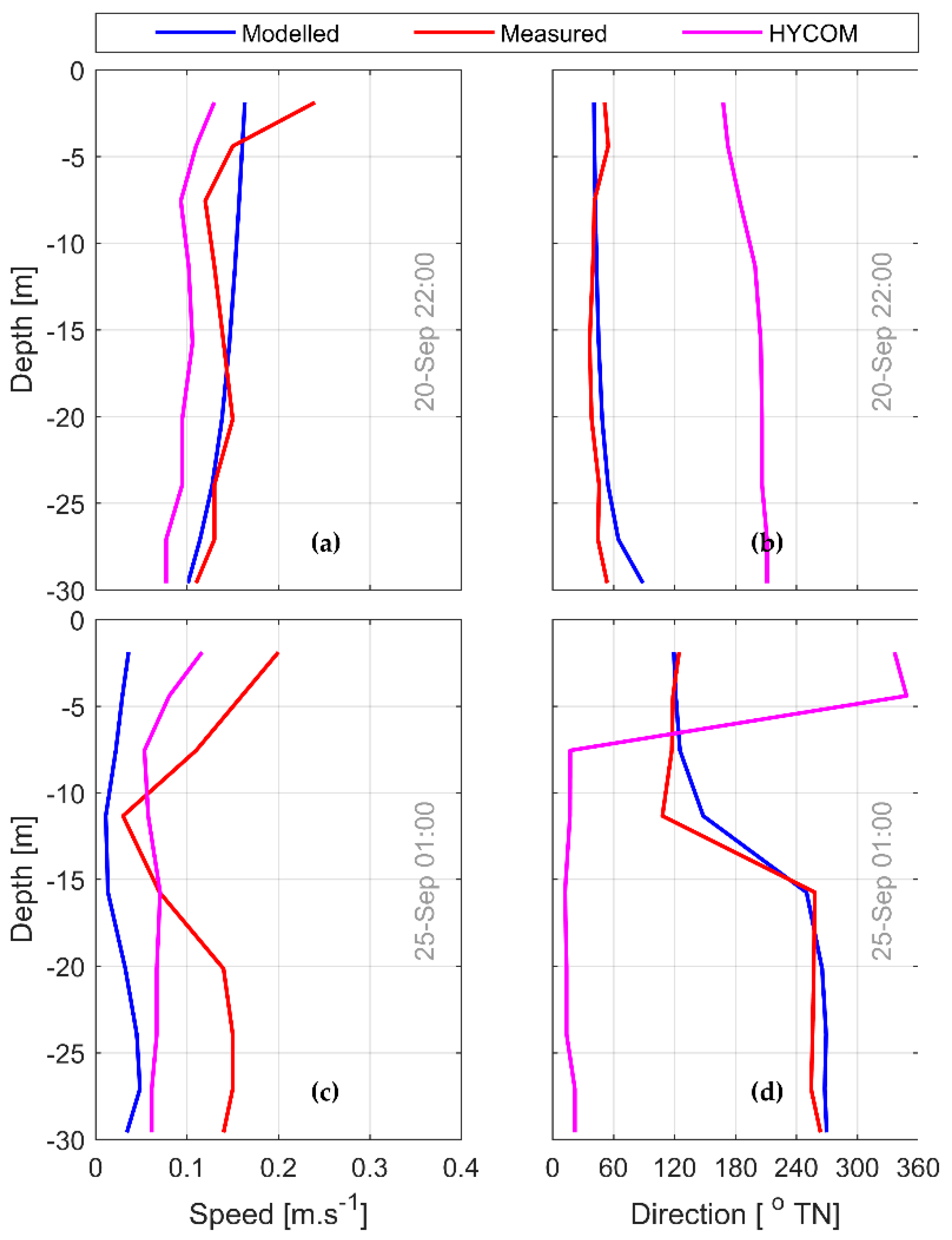
Finally, while calibration was not performed in the vertical sense, vertical profiles as produced by the final HRM configuration were investigated. All three products were interpolated to the HRM vertical grid for fair comparison. In most cases the vertical velocity profile is reasonably well reproduced, though there are occasions where both models fail to simulate reversals at certain depths. These cases are few and far between for the calibration period, however. Figure 3a,b show the case of a homogenous vertical profile. Figure 3c,d show the case of a directional reversal (~150°) with depth roughly between 11 and 15 m, which is well simulated by the HRM and absent from the coarse global model. It should be borne in mind that currents are weak and variable throughout the simulation period, however, and are therefore likely to exhibit higher relative variability.
It should be noted that the limited spatial and temporal coverage of available in situ measurements poses a challenge to the robust calibration of coastal models. While gridded satellite products provide wide geographical coverage, their spatial and temporal resolutions (typically 0.05–0.25°, daily mean) render them unsuitable for use as objective calibration/validation references. For example, in the present study, differences in daily mean SSTs between the HRM and the OSTIA v2 blended product [92] fell within OSTIA’s estimated error for the HRM domain.
3.4. HRM Validation Performance
Validation results, compiled by assessing model performance at different times or places to those assessed for calibration, are presented in Table A4 in Appendix A. The validation process confirms that the HRM performs similarly outside of the calibration space and time. Since calibration was not performed on wave, temperature and salinity parameters, they are included in this validation assessment.
Figure 4 shows validation results for near-bottom current velocities just north of the Port of Cape Town (CU3) and a point between Robben Island and the mainland (CU2). Corresponding time series plots are available as supplementary material (Figures S5 and S6). Prominent, regular oscillatory features evident in these areas were confirmed to be tidal by means of frequency analysis, which reveals that the energy spectrum in the HRM is dominant at frequencies of 1.938 and 2.0 cycles per day (cpd). These correspond to the M2 (1.932 cpd) and S2 (2.0 cpd) tidal constituents [76]. This is likely related to the importance of tidal and inertial oscillation in the absence of strong atmospheric forcing. The HRM simulates these faithfully but may be missing some other sub-grid scale processes, which in the context of these near-stagnant flows, become relevant. The benefit of increased resolution is clear in the reproduction of the directional signal. Two relatively strong east-south-eastward flow events, peaking during the mornings of the 2nd and 10th September, are underestimated. Inspection of wind signals suggests that this might be a missed bottom return-flow mechanism in response to north-westward flow driven by strong south-easterly wind events (with a lag time of approximately 8 h).
Current speeds and directions produced by the HRM are generally in better agreement with measurements, but are unable to simulate some high frequency variability. While much of the focus of the calibration and validation has centred on Table Bay due to the availability of data, Figure 5 provides a glimpse into the solution in the north-eastern reaches of False Bay, near Gordon’s Bay (site CU4). Corresponding time series plots are available in the supplementary material (Figures S7 and S8). Here, zonal surface flows are faithfully reproduced and slightly outperform HYCOM. Both the HRM and HYCOM overestimate northward flows and underestimate southward flows, with these inaccuracies greater in the HRM. HRM mean speeds and directions were 7.4 × 10⁻² m s−1 and 164.9° TN, compared to corresponding measured currents of 6.7 × 10⁻² m s−1 and 176.6° TN for a 24-day comparison. Near the bed, modelled and measured speeds and directions were 4.6 and 4.5 × 10⁻² m s−1, and 188.0 and 174.2° TN, respectively. Near Simon’s Town, mean HRM speeds and directions were 4.0 × 10⁻² m and 224.1° TN. Corresponding measurements were 8.7 × 10⁻² m and 238.0° TN. Time series plots for this site are available in supplementary material (Figure S9). At both Gordon’s Bay and Simon’s Town, these results represent an improvement over corresponding HYCOM means (refer to Table A4).
Comprehensive temperature and salinity data were mostly unavailable for the study period, precluding their inclusion in calibration and preventing meaningful validation. Several snapshot temperature and salinity profiles were available from the World Ocean Database; however. Figure 6 shows snapshot comparisons between measured profiles and the closest matching model profiles in space and time at three different points in the study domain. Both the HYCOM and measured profiles are linearly interpolated to the HRM grid for fair comparison. These comparisons provide, at best, limited insight into model performance, given the instantaneous nature of the measurement and little available information regarding measurement accuracy. South of Cape Point (TS4), modelled temperatures and salinities from the HRM agree closely with measurements, with RMSEs of 0.89 °C and 0.13 ppt, respectively, in a water column of more than 80 m. This represents an improvement over the global model, which produces RMSEs of 2.76 °C and 2.48 ppt. Surface temperatures agree very closely, with sensitivity tests revealing this to be the result of including surface heat flux forcing. In the shallows of False Bay near Gordon’s Bay (TS5), surface temperatures are again accurately simulated, but the HRM fails to produce a slight warming between 2 and 7 m, and a cooling thermocline below 15 m. The limitations of model bathymetric resolution are made clear here, with the HYCOM model only producing results to a depth of between 10 and 15 m. West of the Peninsula (TS9), the HRM reproduces the shape of the temperature and salinity curves, but a constant overestimation throughout the water column is evident. Preliminary testing revealed the potential in the correction of temperature and salinity boundary condition biases towards improving these results, though a full appraisal in this regard is beyond the scope of the present study. Though robust validation of GOFS 3.1 temperature and salinity in this area is lacking, Ref. [38] determined the product to show a 38% agreement in SST with radiometer measurements at a near-co located point within False Bay, and tending generally to overestimate. Furthermore, during data assimilation experiments with a research HYCOM configuration, Refs. [93,94] noted warm SST biases in the Benguela region, which are exacerbated by the assimilation of sea-level anomaly data (GOFS 3.1 assimilates sea surface height data). Sub-surface validation of GOFS 3.1 temperatures and salinities is lacking, but these studies point to the possibility of biases in HYCOM temperature boundary conditions which might propagate into the HRM domain. Another noticeable feature is the similarity between the HYCOM and HRM profiles. This is due to the proximity of the profile location to the HRM model boundary. Similar plots to those in Figure 6 were produced for all available measured profiles (and their basic performance metrics given in Table A3).
3.5. Circulation and Density Dynamics
A brief commentary is provided on the development of broad circulation and density patterns. Commentary is focused around south-easterly and north-westerly wind events, since these are common synoptically driven scenarios. For the August-October 2006 simulation period, 23 (6) such south-east (north-west) events (with wind speed > 7 m s−1) occurred during the simulation period. Overall, wind directions in the south-east and north-west quadrants were equally prevalent, at 47% of the period each (total 94%, with 6% north-easterly and south-westerly directions). For the August-October 2010 simulation, 21 (14) south-east (north-west) events with wind speeds > 7 m s−1 occurred. Overall, south-east (north-west) winds occurred 42 (48)% of the time.
3.5.1. Flow under South Easterly Wind Events
Several south-easterly events were inspected in terms of the hydrodynamic response. The expectations established by the literature are qualified in that while previously observed response features are produced by the HRM, these features do not always occur in response to similar forcing. An expected result is relatively strong westward flow south of False Bay, becoming north-westward along the south-western coastline of the Cape Peninsula, with little vertical shear (Figure 7). Offshore of Olifantsbos and extending as far as Table Bay; however, surface flows continue to the north-west while bottom flows turn eastward, presumably to balance the surface divergence. Flow speeds decrease north of Oudekraal, with weak northward flow between Oudekraal and the northern extent of the study domain, even under relatively strong south-easterly wind events. Velocity maxima appear regularly in the vicinity of prominent headlands; for example, near Cape Hangklip, Cape Point and Slangkop. Close inspection of Table Bay reveals weak northward drift under south-easterly winds (Figure 8), but this needs further qualification (discussed later in this section). Water is seen entering between Green Point and Robben Island, and exiting between Robben Island and the mainland. This agrees with the observations of a so-called “anticyclonic” flow under south-easterly winds by Ref. [5]. Surface and bottom flows were similar in Table Bay, with little evidence of significant vertical shear.
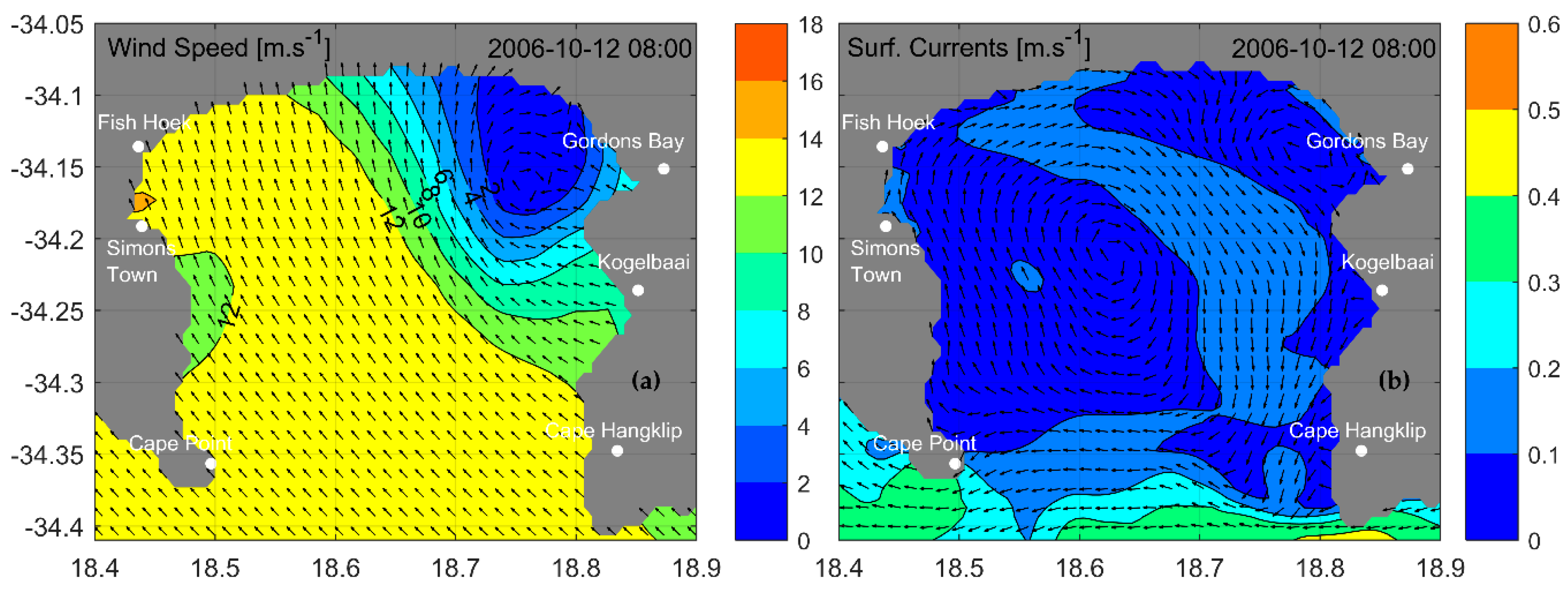
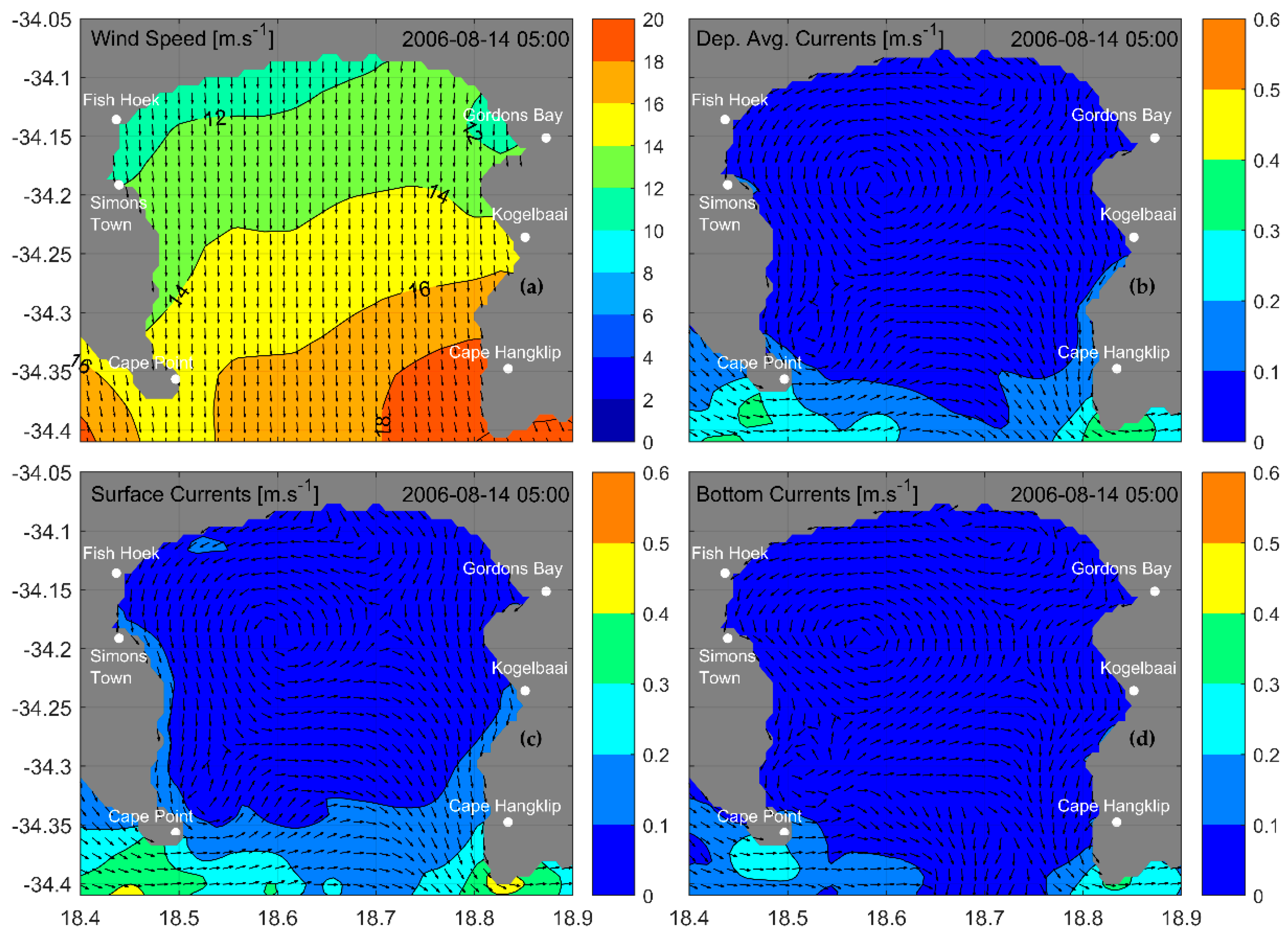
Within False Bay, cyclonic flow is produced in response to south-easterly winds. However, the development of this circulation appears more nuanced than previously thought. First, cyclonic flow is not guaranteed during all south-easterly wind events, with weak, variable, and eddying flow developing during some of these. Weak, anticyclonic eddies of this nature are frequently noted near Gordon’s Bay and Kogelberg. Net cyclonic flow appears more likely to be permitted when the north-eastern margins of the Bay (in the vicinity of Gordon’s Bay) are sheltered from the south-easterly winds by the steep topography near the coast (Figure 9). Second, when winds are stronger or more easterly, speeds may increase in the north-eastern margins of the Bay and the wind shadow is overcome. This induces a westward flow in the northern margins which is able to dominate, imparting a net anti-cyclonic pattern for the Bay (Figure 10). Finally, poleward motion, as observed by Ref. [35] at both Cape Point and Cape Hangklip was noted at times during south-easterly winds. This appeared to be more likely during times when the wind shadow was absent from the north-eastern margins.
Outside of False Bay, currents rarely exceeded 0.6 m s−1, being strongest in a band between Onrus and south of the zonal mid-point across the mouth of False Bay (during ESE winds) and in the regions of the prominent headlands at Cape Hangklip, Cape Point and Slangkop (during SE winds). Within False Bay, velocities rarely exceeded 0.2 m s−1, except in the extreme northerly reaches, where wave-driven currents of up to 0.4 m s−1 were noted. Throughout the study periods and for False Bay, the western seaboard and Table Bay, coherent flow patterns only developed under winds speeds higher than approximately 12 m s−1. With lighter winds, even in steady directions, flow directions appeared haphazard, and speeds negligible (mainly < 0.1 m s−1, reaching 0.2 m s−1).
3.5.2. Flow under North-Westerly Wind Events
Under north-westerly winds, two noteworthy features emerge, the rest being transient, weak and variable. The first is strong south-eastward flow, starting a few kilometres north-west of Cape Point, becoming eastward after rounding Cape Point (Figure 11) and extending to the south-eastern corner of the HRM domain. Bottom flows (now south-westward except in the shallow, nearshore band) between Oudekraal and Olifantsbos are nearly opposed to surface flows (now south and south-eastward).
The second are the flow patterns within False Bay. An example of the anticyclonic rotation observed in the literature is shown in Figure 12, having developed during northerly wind conditions on the morning of 14 August 2006. This rotation is weak, with flows barely exceeding 0.3 m s−1 near Cape Point and remaining below 0.2 m s−1 across the rest of the Bay. Poleward flow developing offshore of Kogelbaai and extending along the south-eastern margins prevents the completion of the pattern; however. Flow is directionally similar throughout the vertical column. Figure 13 shows southward and south-eastward surface flow (aligned with the wind) having developed during a different north-westerly wind event. Weak north-westward bottom return flows occur, and no noticeable gyre-circulation develops. In such cases, there is no dominant depth-integrated pattern, given the vertical shear.
In Table Bay, an interesting feature develops in response to large wave events (>3 m reaching the region west of Robben Island). This is the generation of a well-developed cyclonic eddy, centred south-east of Robben Island, as shown in Figure 14b. Eastward flow is induced, possibly aided by westerly wind stresses which often accompany the onset of large wave events, causing a local acceleration along the southern and south-eastern margins of Robben Island. This imparts cyclonic vorticity, aided by bathymetry and the nearby mainland coastline. The eddy was observed to persist until significant wave heights subsided west of Robben Island. The cyclonic eddy is sometimes accompanied by a weak, anti-cyclonic eddy centred north-west of Robben Island. When the cyclonic eddy is in operation, part of the eastward flow in the lee of Robben Island and along its northern shores is deflected northwards, creating a near-shore divergence at Bloubergstrand. The eddy was confirmed to be a wave-driven Eulerian circulation after the same configuration, run without wave coupling, failed to produce the feature on any occasion (Figure 14d). Moreover, north-westerly winds (frequently associated with cold frontal passage and stormy conditions) are by themselves insufficient to produce the feature if the associated waves are insufficiently large. In this case, a general southward drift develops in the Bay, in agreement with the so-called clockwise rotation observed by Ref. [5]. The eddy is distinct from this general clockwise circulation, however. The general southward drift was observed to produce flow directions ranging between 090 and 270°. The eddy produced in the HRM is a closed structure, with flow in the north-western quadrant being northwards and north-eastwards. The northward deflection of the eastward flow in the lee of Robben Island; not noted in the general drift case; and its dependency on wave conditions (rather than wind direction) also suggest it is a different regime.
3.5.3. Horizontal Temperature Distributions
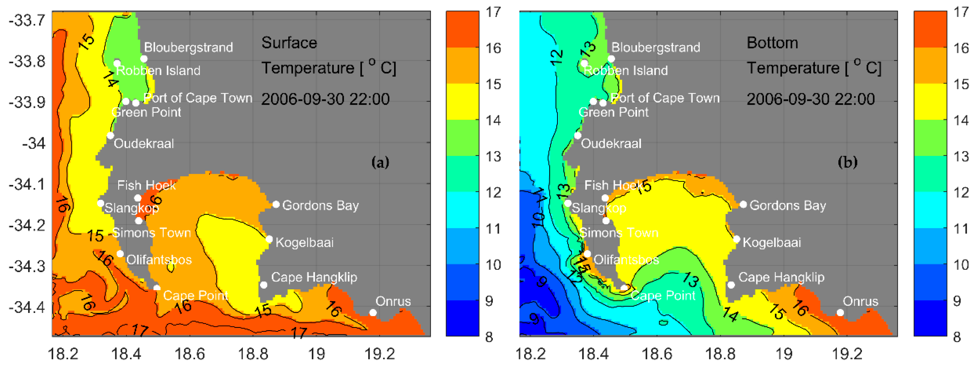
Inspection of surface and bottom temperature fields in conjunction with wind reveals some broad characteristics of the horizontal temperature distributions produced by the HRM. Immediately west of the Cape Peninsula, cold water, first evident in deeper layers, appears at the surface in response to upwelling favourable wind events. This mechanism acts as one of the main drivers of near-coast temperature dynamics, but its effect is translated to other areas of the model domain via wind-driven advection. For most of the modelled period, there is a distribution of cold (8–12 °C) bottom water extending southwards from north of Table Bay, along the western seaboard. It rounds Cape Point, spreading eastwards south of False Bay, as far as 18.8° E. This provides a reliable supply of cold water to be upwelled against the Cape Peninsula during favourable winds, particularly at Slangkop and Oudekraal. The failure of the tongue of cold bottom water to extend beyond about 18.8° E is a possible reason for the lack of strong upwelling events in the vicinity of Cape Hangklip which, though observed in the literature, did not materialize strongly in these results. This might be due to the simulation periods being too early (spring-early summer) to produce upwelling at Hangklip, which is typically noted during mid-summer months. Figure 15 clearly shows the onset of a typical upwelling event centered off Slangkop and Oudekraal, the supply of cold bottom waters to the west and south-west, and False Bay still exhibiting thermal uniformity characteristic of its winter configuration. The upwelled centres off Slangkop and Oudekraal will ultimately join and spread along much of the western Peninsula, with the 10 °C isotherm reaching the surface within 24 h.
Periods with westerly and northerly component winds allow warmer surface waters (up to 15 °C) to move close to the coast along the west coast (north of Table Bay) and along the western Cape Peninsula. While these winds prevent warmer waters along the southern boundary from entering False Bay, they are insufficient to induce any sort of upwelling along the western and northern shores of the Bay. When these winds relax, or are replaced by southerly component winds; however, warmer waters of up to 16.5 °C, presumably of Agulhas origin, are advected into False Bay.
Moderate (max ~10 m s−1) westerly and north-westerly winds, starting late on the 29 September 2006 and lasting for just less than 3 days produced an example of this slight surface warming along the western Peninsula, as shown in Figure 16.
3.5.4. Density Structure
To assess the evolution of the density structure, several vertical zonal and meridional cross sections were defined. Density dynamics appear strongly temperature controlled, with salinity exhibiting little variability throughout the domain. This result is in agreement with observations from Ref. [4] west of the Peninsula and Ref. [37] in False Bay. Brief remarks are made regarding temperature dynamics and upwelling at the various centres mentioned in the literature.
At Slangkop, the development of coastal upwelling is clearly illustrated following a series of south-easterly wind events in late August 2006. Prior to the onset of the wind events, surface temperatures decrease slightly from 15–16 °C at the western model boundary to 13–14 °C at the coast (Figure 17a). Near the western boundary, below 75 m, temperatures are 10 °C. The thermocline is well-developed offshore, whereas coastwards of the 50 m isobath, the water column is better mixed and warmer. When south-easterly winds begin to blow, the thermocline is pulsed, and shoaling starts to occur coastwards (Figure 17b). The thermocline continues to pulse and shoal, until the 10 °C isotherm breaks the 50 m contour, and the surface is at 11.0 °C near the coast. These cold surface conditions persist after the deterioration of the south-easterly wind event, through light and variable conditions, for more than two days. Ultimately, the arrival of a moderate north-westerly wind event re-establishes vertical stratification by advecting warm surface waters towards the coast. While not as pronounced as the upwelling event, the strong north-westerly wind event mentioned previously (early October 2006) did result in downwelling at the coast. A warm pool of 13.5–14.5 °C surface water moves towards the coast, displacing the previously shoaling thermoclines 13 °C and colder. A zonal section at Oudekraal, the second main upwelling centre along the Peninsula, reveals similar behaviour. To assess the time-varying evolution of stratification, Hovmöller diagrams of Brunt–Väisälä frequency were constructed for nearshore, mid-range and offshore water column profiles (Figure S10, Supplementary Material). The location of the profiles is indicated by dashed grey lines in Figure 17. For all three profiles, shallow stratification and episodic vertical mixing were evident throughout the simulation period, with the intensity of stratification increasing markedly from the 15th of September. Stratification was strongest and most stable at the offshore profile.
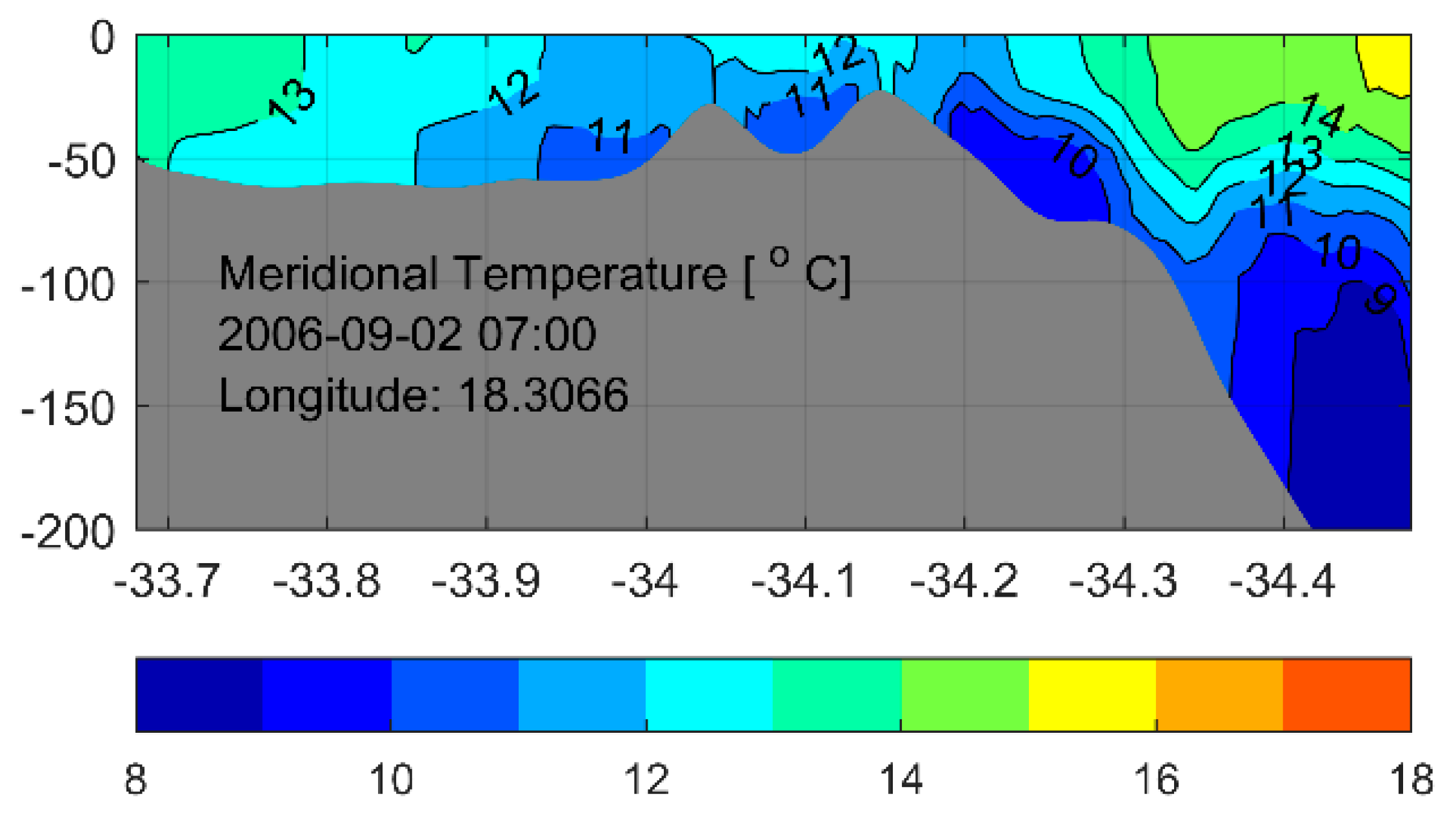
Further north, across a zonal section in Table Bay at 33.867° S, minimal evidence of active upwelling is noted, despite temperatures being uniformly cold (down to 10.5 °C) following strong south-easterly winds. The Bay exhibits little stratification. This suggests that the origins of cold water in Table Bay are upwelling centres elsewhere; either to the north, at Cape Columbine or south, at Oudekraal. This explanation is strengthened by the appearance of warm and cold pools of water away from boundaries in the zonal cross-section and is consistent with the mainly meridional flow in the area. Towards the northern reaches of the Bay, a cross-section across Robben Island at 33.807° S reveals weak upwelling against the western rise of Robben Island. Cold water isotherms do not break the surface; however, and little evidence of upwelling appears along the west coast of the mainland at the same latitude. A meridional section between the Port of Cape Town, through Table Bay and to the northern model boundary confirms that during south-easterly wind events, cold water (~10.5–11 °C) enters the Bay from the south, most likely from the upwelling tongue along the western seaboard. This prompted inspection of a meridional section extending from the northern model boundary to the southern at 18.307° E (Figure 18). Along the southern part of this section, frequent pulsing of the thermocline against the rising bathymetry south-west of Cape Point results in cold water from deep, off-shelf regions being pushed up and on to the shelf. This water sometimes pools with cold, deep water entering from the west between Cape Point and Slangkop, and again further north between Oudekraal and Table Bay. These results suggest that the primary sources of cold water for coastal upwelling are the western and south-western regions of the domain. While the possibility of a southward supply from the upwelling centre of Cape Columbine to the north of the domain is not precluded, it is not strongly evident here. During north-westerly winds, warmer water from the north-west progressively fills the Bay uniformly in the vertical.
In False Bay during winter, the vertical structure is fairly uniform and exhibits low variability, remaining mostly between 13 and 14.5 °C. Inspection of Hovmöller diagrams of Brunt–Väisälä frequency at nearshore, mid-bay and near-mouth profiles, along a meridional transect down the middle of the Bay, revealed that if stratification develops during late winter, it is confined to the very near-surface in the northern margins (Figure S11, Supplementary Material). This is likely the result of solar heating. From late September, relatively stronger (though still moderate) episodic stratification is evident, though it is quickly broken down. An example is shown in Figure 19. This is likely the result of strong winds during summer and mixing due to waves. This agrees with Ref. [38], who noted temperature within the Bay to be strongly linked to waves. In the middle of the Bay during late October, the entrainment of colder waters from deeper offshore regions results in strongly stratified mid-depth layers. This entrainment is unable to progress beyond the middle regions of the Bay; however, and remains below about 20 m, leaving the surface layers mixed and warm and the bottom layers mixed and cool. An example of such an event is evident for late October in Figure S11b (Supplementary Material).
4. Conclusions
The coastal oceans of the Cape Peninsula are key natural resources supporting a multitude of human and ecological interests. As such, robust understanding of, and the ability to simulate their evolution are required.
This study presents a coupled wave and flow numerical high-resolution model (HRM) which was built for this purpose. It includes the most important physical processes identified in the literature, and calibration and validation indicate that the model reproduces the mean circulation and dynamical features. Comparison of HRM and HYCOM RMSEs demonstrates the value in downscaling information from global-scale systems towards the coast. While the HRM does not universally increase accuracy (a partial symptom of limited calibration/validation data, with possible contributions from errors in surface and boundary forcing), it offers the distinct advantage of greatly increasing the spatial density of information near the coast.
Averaged HRM current speeds and directions agree well with measurements, while high frequency variability (such as rapid speed increases or directional reversals) is unresolved at times. However, a deficiency of observations makes validation difficult, and performance metrics should be read with this limitation in mind. Following the literature, a range of expected dynamical behaviour is reproduced. Flow speeds in the expected range are produced for False Bay, the western Peninsula and Table Bay. Key features such as coastal upwelling at Slangkop and Oudekraal, and vertical shear in currents are simulated. While vertical temperature and salinity profiles are generally well reproduced, there is evidence that boundary condition biases in these quantities could be propagating into the high-resolution model. While this is especially evident near the open boundaries, the effect may manifest further into the model. A sensitivity test revealed the importance of surface heat fluxes for False Bay sea temperatures.
Commentary on the evolution of the circulation revealed some novel findings which add to the body of knowledge for this region. The study qualifies the expectation of anticlockwise circulation in False Bay by noting poleward flow near Kogelbaai, which prevents true anticyclonic flow across the whole Bay. The expectation of cyclonic flow in False Bay during south-easterly winds is also qualified. First, cyclonic flow does not always develop during south-easterly winds. Second, it is more likely to be permitted when the wind shadow near Gordon’s Bay is in effect. Third, when this wind shadow breaks down, an anticyclonic rotation, induced by strong westward flow along the north-eastern reaches, is established. Along the western Peninsula, expected results of wind-aligned surface flows and opposite deep flows, are achieved. In Table Bay, the general northward (southward) drift under south-easterly (north-westerly) winds described by Ref. [5] are replicated. However, a coherent cyclonic eddy, distinct from this circulation and generated by large wave conditions, is also described.
The HRM demonstrates potential utility for interdisciplinary coastal studies. With further development it is also suitable for deployment in an operational mode, as has been successfully done with similar architecture. The study is constrained by limited calibration and validation data. Suggested future work therefore includes further model testing when observations become available, a detailed investigation of the wave-current interactions in Table Bay, and deeper analysis of the effects of heat-flux forcing, waves and tides on False Bay’s vertical density structure. Running the model for mid-summer and mid-winter periods would also allow for better understanding of the seasonal variability.
Supplementary Materials
The following are available online at https://0-www-mdpi-com.brum.beds.ac.uk/article/10.3390/jmse9040359/s1, Figure S1: SLP Forcing Validation, Figure S2: Wind Forcing Validation, Figure S3: Near-Surface Current Velocity Timeseries at CU1, Figure S4: Near-Bottom Current Velocity Timeseries at CU1, Figure S5: Near-Bottom Current Velocity Timeseries at CU2, Figure S6: Near-Bottom Current Velocity Timeseries at CU3, Figure S7: Near-Surface Current Velocity Timeseries at CU4, Figure S8: Near-Bottom Current Velocity Timeseries at CU4, Figure S9: Near-Bottom Current Velocity Timeseries at CU5, Figure S10: Vertically Integrated Brunt-Väisälä Frequency near Slangkop, Figure S11: Vertically Integrated Brunt-Väisälä Frequency in False Bay.
Author Contributions
Conceptualization, M.d.V. and C.R.; Formal analysis, M.d.V.; Funding acquisition, C.R. and M.V.; Investigation, M.d.V.; Methodology, M.d.V. and C.R.; Project administration, M.d.V., C.R. and M.V.; Resources, C.R.; Software, M.d.V. and C.R.; Supervision, C.R. and M.V.; Validation, M.d.V.; Visualization, M.d.V.; Writing—original draft, M.d.V.; Writing—review & editing, M.d.V., C.R. and M.V. All authors have read and agreed to the published version of the manuscript.
Funding
This work was partially supported by the National Research Foundation of South Africa (grant number 118754)—South Africa–Norway cooperation on ocean research including blue economy, climate change, the environment and sustainable energy (SANOCEAN).
Institutional Review Board Statement
Not applicable.
Informed Consent Statement
Not applicable.
Data Availability Statement
This study makes use of various data sets with different availability. HRM model data may be made available on request from the corresponding author. The data are not publicly available due to funding restrictions. 3rd party data used include wave and current measurements, obtained from the Council for Scientific and Industrial Research (CSIR) and Transnet National Ports Authority (TNPA), water level measurements, obtained from the South African Navy Hydrographic Office (SANHO) and wind measurements from the South African Weather Service.
Acknowledgments
The authors would like to acknowledge the following people and entities for supporting this work: The Transnet National Ports Authority (TNPA) for the use of current and wave measurement data. The South African National Hydrographic Office (SANHO) for the use of water level and bathymetric data. The Council for Scientific and Industrial Research (CSIR) for the use of current measurement data. The Climate Systems Analysis Group (CSAG) for the use of the WASA wind forcing data. The South African Weather Service (SAWS) for the use of wind and pressure measurement data.
Conflicts of Interest
The authors declare no conflict of interest.
Appendix A

Table A1.
Summary of validation statistics for the wind and pressure forcing applied to the HRM. Refer to Figure 1 for location references. Wind direction error metrics are not true RMSEs, but rather a mean angular difference for the entire time series.
Table A1.
Summary of validation statistics for the wind and pressure forcing applied to the HRM. Refer to Figure 1 for location references. Wind direction error metrics are not true RMSEs, but rather a mean angular difference for the entire time series.
| Sea Level Pressure | Validation Time Period | Reference Data Description | Location Reference | RMSE (hPa) | |
| 1 August 2006 00:00–30 October 2006 21:00 | RCYC AWS | W1 | 1.5077 | ||
| Robben Island AWS | W2 | 1.0932 | |||
| Strand AWS | W4 | 1.9382 | |||
| 1 August 2010 00:00–30 October 2010 21:00 | RCYC AWS | W1 | 1.6044 | ||
| Robben Island AWS | W2 | 2.1458 | |||
| Strand AWS | W4 | 1.7438 | |||
| Wind | Validation Time Period | Reference Data Description | Location Reference | RMSE | |
| Speed (m s−1) | Direction (°) | ||||
| 1 August 2006 00:00–30 October 2006 21:00 | RCYC AWS | W1 | 2.916 | −21.984 | |
| Robben Island AWS | W2 | 3.403 | 8.230 | ||
| Strand AWS | W4 | 4.086 | −5.699 | ||
| 1 August 2010 00:00–30 October 2010 21:00 | RCYC AWS | W1 | 2.916 | −21.984 | |
| Robben Island AWS | W2 | 3.403 | 8.230 | ||
| Strand AWS | W4 | 4.086 | −5.699 | ||
| Cape Point AWS | W5 | 3.436 | 19.367 | ||
| Slangkop AWS | W6 | 2.740 | 1.040 | ||
Table A2.
Summary of water level and current performance statistics after the iterative calibration of the HRM, using the final parameterisation settings (see Table 1).
Table A2.
Summary of water level and current performance statistics after the iterative calibration of the HRM, using the final parameterisation settings (see Table 1).
| Water Level | Calibration Time Period | Reference Data Description | Location Reference | RMSE (m) | |||
| 1 August 2006 00:00–30 October 2006 21:00 | Cape Town tide gauge | WL1 | 0.205 | ||||
| Simon’s Town tide gauge | WL2 | 0.102 | |||||
| Current Velocity | Calibration Time Period | Reference Data Description | Location Reference | RMSE (m s−1) | |||
| HRM | HYCOM | ||||||
| u | v | u | v | ||||
| 25 August 2006 09:00–27 September 2006 09:00 | Table Bay ADCP | CU1 (near surface) | 0.080 | 0.100 | 0.105 | 0.097 | |
| CU1 (near bottom) | 0.073 | 0.064 | 0.066 | 0.057 | |||
Table A3.
Mean current speeds and directions for all possible co-located HRM, HYCOM and measurement site for the duration of their overlap. In the last two columns on the right, green cells indicate closer agreement between the modelled (HRM or HYCOM) and measured mean parameter.
Table A3.
Mean current speeds and directions for all possible co-located HRM, HYCOM and measurement site for the duration of their overlap. In the last two columns on the right, green cells indicate closer agreement between the modelled (HRM or HYCOM) and measured mean parameter.
| Site (Type) | Mean Current Parameters for Overlapping Period | HRM | HYCOM | Measured | ||
|---|---|---|---|---|---|---|
| CU1 (calibration) | near surface (m s−1) | 0.088 | 0.074 | 0.128 | 0.04 | 0.05 |
| near bottom (m s−1) | 0.058 | 0.045 | 0.077 | 0.02 | 0.03 | |
| near surface (°) | 74.8 | 218.8 | 96.5 | 21.8 | 121.9 | |
| near bottom (°) | 121.9 | 126.1 | 145.1 | 23.2 | 18.9 | |
| CU2 (validation) | near bottom (m s−1) | 0.077 | 0.016 | 0.106 | 0.03 | 0.09 |
| near bottom (°) | 295.8 | 271.9 | 275.2 | 20.7 | 3.2 | |
| CU3 (validation) | near bottom (m s−1) | 0.047 | 0.010 | 0.070 | 0.02 | 0.06 |
| near bottom (°) | 108.9 | 266.5 | 133.3 | 24.4 | 133.2 | |
| CU4 (validation) | near surface (m s−1) | 0.074 | 0.048 | 0.067 | 0.01 | 0.02 |
| near bottom (m s−1) | 0.046 | 0.033 | 0.045 | 0.00 | 0.01 | |
| near surface (°) | 164.9 | 222.7 | 176.6 | 11.7 | 46.0 | |
| near bottom (°) | 188.0 | 237.3 | 174.2 | 13.8 | 63.1 | |
| CU5 (validation) | near bottom (m s−1) | 0.040 | 0.019 | 0.087 | 0.05 | 0.06 |
| near bottom (°) | 224.1 | 153.8 | 238.0 | 13.9 | 84.2 |
Table A4.
Summary of validation statistics. These statistics are produced for all relevant parameters for times and places where measurements were available, excluding those used during calibration.
Table A4.
Summary of validation statistics. These statistics are produced for all relevant parameters for times and places where measurements were available, excluding those used during calibration.
| Water Level | Validation Time Period | Reference Data Description | Location Reference | RMSE (m) | |||
| 1 August 2010 00:00–22 October 2010 21:00 | Cape Town tide gauge | WL1 | 0.039 | ||||
| Simon’s Town tide gauge | WL2 | 0.158 | |||||
| Current Velocity | Validation Time Period | Reference Data Description | Location Reference | RMSE (m s−1) | |||
| HRM | HYCOM | ||||||
| u | v | u | v | ||||
| 27August 2006 11:00–27 September 2006 06:00 | Table Bay SeaPac 1 | CU2 (near bottom) | 0.060 | 0.078 | 0.082 | 0.101 | |
| 27August 2006 11:00–03 October 2006 03:00 | Table Bay SeaPac 2 | CU3 (near bottom) | 0.044 | 0.048 | 0.070 | 0.049 | |
| 20 August 2010 11:00–13 September 2010 09:00 | Gordon’s Bay ADCP | CU4 (near surface) | 0.057 | 0.088 | 0.053 | 0.049 | |
| CU4 (near bottom) | 0.044 | 0.046 | 0.032 | 0.049 | |||
| 29 September 2010 11:00–22 October 2010 08:00 | Simon’s Town SeaPac | CU5 (near bottom) | 0.057 | 0.071 | 0.043 | 0.105 | |
| Temperature (T)/Salinity (S) | Validation Time Period | Reference Data Description | Location Reference | RMSE | |||
| HRM | HYCOM | ||||||
| T (°C) | S (ppt) | T (°C) | S (ppt) | ||||
| 26 October 2006 10:30:59 | WOD Cast ID # 17365255 | TS4 | 0.89 | 0.13 | 2.76 | 2.48 | |
| 26 October 2006 13:57:59 | WOD Cast ID # 17365256 | TS5 | 1.57 | 0.08 | 1.20 | 0.21 | |
| 26 October 2006 17:17:59 | WOD Cast ID # 17365257 | TS6 | 2.08 | 0.15 | 3.40 | 0.30 | |
| 28 October 2006 11:00:59 | WOD Cast ID # 17365268 | TS7 | 1.29 | 0.16 | 1.29 | 0.16 | |
| 29 October 2006 17:32:59 | WOD Cast ID # 17365280 | TS8 | 3.14 | 0.32 | 3.50 | 0.37 | |
| 29 October 2006 18:14:00 | WOD Cast ID # 17365281 | TS9 | 3.57 | 0.34 | 3.57 | 0.35 | |
| 29 October 2006 18:49:00 | WOD Cast ID # 17365282 | TS10 | 3.58 | 0.38 | 4.55 | 0.45 | |
| 1 September 2010 08:19:00 | WOD Cast ID # 13192128 | TS11 | 0.15 | 0.13 | 0.91 | 0.13 | |
| Waves | Validation Time Period | Reference Data Description | Location Reference | RMSE | |||
| Hs (m) | Tp (s) | Dp (°) | |||||
| 1 August 2006 00:00–30 October 2006 21:00 | TNPA Wave Rider Buoy | WV1 | 0.49 | 1.45 | 10.80 | ||
References
- Salonen, N.M. Towards Rogue Wave Characterization in False Bay, South Africa. Master’s Thesis, University of Cape Town, Cape Town, South Africa, 2019. [Google Scholar]
- Day, J.H. The biology of false bay, South Africa. Trans. R. Soc. S. Afr. 1970, 39, 211–221. [Google Scholar] [CrossRef]
- de Vos, M.; Rautenbach, C. Investigating the connection between metocean conditions and coastal user safety: An analysis of search and rescue data. Saf. Sci. 2019, 117, 217–228. [Google Scholar] [CrossRef]
- Shannon, L.V.; Nelson, G.; Jury, M.R. Hydrological and Meteorological Aspects of Upwelling in the Southern Benguela Current. In Coastal Upwelling; Richards, F.A., Ed.; American Geophysical Union: Washington, DC, USA, 1981; Volume 1, pp. 39–43. ISBN 9781118665329. [Google Scholar]
- Van Ieperen, M.P. Hydrology of Table Bay; Final Report; Department of Oceanography, University of Cape Town: Cape Town, South Africa, 1971. [Google Scholar]
- Quick, A.J.R.; Roberts, M.J. Table Bay, Cape Town, South Africa: Synthesis of available information and management implications. S. Afr. J. Sci. 1993, 89, 276–287. [Google Scholar]
- Pfaff, M.C.; Logston, R.C.; Raemaekers, S.J.P.N.; Hermes, J.C.; Blamey, L.K.; Cawthra, H.C.; Colenbrander, D.R.; Crawford, R.J.M.; Day, E.; du Plessis, N.; et al. A synthesis of three decades of socio-ecological change in False Bay, South Africa: Setting the scene for multidisciplinary research and management. Elementa 2019, 7, 32. [Google Scholar] [CrossRef] [Green Version]
- Gründlingh, M.L.; Hunter, I.T.; Potgieter, E. Bottom currents at the entrance to False Bay, South Africa. Cont. Shelf Res. 1989, 9, 1029–1048. [Google Scholar] [CrossRef]
- Harris, T.F.W. Review of Coastal Current in Southern African Waters. National Scientific Programmes Unit, CSIR. 1978. Available online: https://researchspace.csir.co.za/dspace/handle/10204/2300 (accessed on 26 June 2020).
- Western Cape Government Provincial Treasury. Provincial Economic Review and Outlook; Western Cape Government Provincial Treasury: Cape Town, South Africa, 2017.
- Celliers, L.; Colenbrander, D.R.; Breetzke, T.; Oelofse, G. Towards increased degrees of integrated coastal management in the city of Cape Town, South Africa. Ocean Coast. Manag. 2015, 105, 138–153. [Google Scholar] [CrossRef]
- Sowman, M.; Sunde, J. Social impacts of marine protected areas in South Africa on coastal fishing communities. Ocean Coast. Manag. 2018, 157, 168–179. [Google Scholar] [CrossRef]
- Ballance, A.; Ryan, P.G.; Turpie, J.K. How much is a clean beach worth? The impact of litter on beach users in the Cape Peninsula, South Africa. S. Afr. J. Sci. 2000, 96, 210–213. [Google Scholar]
- Munien, S.; Gumede, A.; Gounden, R.; Bob, U.; Gounden, D.; Perry, N.S. Profile of visitors to coastal and marine tourism locations in cape town, South Africa. Geoj. Tour. Geosites 2019, 27, 1134–1147. [Google Scholar] [CrossRef]
- Van Ballegooyen, R. Ben Schoeman Dock Berth Deepening Project Integrated Marine Impact Assessment Study; Council for Scientific and Industrial Research: Stellenbosch, South Africa, 2007. [Google Scholar]
- Potgieter, L.; Goedhals-gerber, L.L. Risk Profile of Weather and System-Related Port Congestion for the Cape Town Container Terminal. S. Afr. Bus. Rev. 2020, 24. [Google Scholar] [CrossRef]
- Colenbrander, D.; Sutherland, C. Reducing the pathology of risk: Developing an integrated municipal coastal protection zone for the City of Cape Town. In Climate Change at the City Scale: Impacts, Mitigation and Adaptation in Cape Town; Cartwright, A., Parnell, S., Oelofse, G., Ward, S., Eds.; Routledge: New York, NY, USA, 2012; pp. 182–201. ISBN 9780203112656. [Google Scholar]
- Boyd, A.J.; Tromp, B.B.; Horstman, D.A. The hydrology off the South African south-western coast between Cape Point and Danger Point in 1975. S. Afr. J. Mar. Sci. 1985, 3, 145–168. [Google Scholar] [CrossRef] [Green Version]
- Tyson, P.D.; Garstang, M.; Swap, R.; Kållberg, P.; Edwards, M. An air transport climatology for subtropical Southern Africa. Int. J. Climatol. 1996, 16, 265–291. [Google Scholar] [CrossRef]
- Jury, M.R. Wind shear and Differential Upwelling Along the South Western tip of Africa. Ph.D. Thesis, University of Cape Town, Cape Town, South Africa, 1984. [Google Scholar]
- Gründlingh, M.L.; Largier, J.L. Fisiese Oseanografie in Valsbaai: ’ n Oorsig. R. Soc. S. Afr. Trans. Trsaac 1988, 47. [Google Scholar]
- Coleman, F. The Development and Validation of a Hydrodynamic Model of False Bay By. Master’s Thesis, Stellenbosch University, Stellenbosch, South Africa, 2019. [Google Scholar]
- CSIR. Effects of Proposed Harbour Developments on the Table Bay Coastline. Report Volume I, ME 1086/1, 1972.
- CSIR. Effects of Proposed Harbour Developments on the Table Bay Coastline. Report Volume 2, ME 1086/2, 1972.
- Schumann, E.H.; Perrins, L.A. Tidal and inertial currents around South Africa. Coast. Eng. 1982, 2562–2580. [Google Scholar]
- Gunn, B.W. The Nearshore dynamics of Matroos Bay-Field and Theoretical Investigations. Master’s Thesis, University of Cape Town, Cape Town, South Africa, 1977. [Google Scholar]
- Gunn, B.W. The Dynamics of Two Cape, Coastal Embayments; Unpublished Report; Department of Oceanography, University of Cape Town: Cape Town, South Africa, 1977; Volume 1. [Google Scholar]
- Taunton-Clark, J.; Kamstra, F. Aspects of marine environmental variability near Cape Town, 1960–1985. S. Afr. J. Mar. Sci. 1988, 6, 273–283. [Google Scholar] [CrossRef] [Green Version]
- Nelson, G.; Polito, A. Information on currents in the cape Peninsula area, South Africa. S. Afr. J. Mar. Sci. 1987, 5, 287–304. [Google Scholar] [CrossRef]
- Atkins, G.R. Camps Bay Outfall Investigation; Institute of Oceanography, University of Cape Town: Cape Town, South Africa, 1965. [Google Scholar]
- Atkins, G.R. Green Point Outfall Investigation; Institute of Oceanography, University of Cape Town: Cape Town, South Africa, 1965. [Google Scholar]
- Andrews, W.R.H.; Hutchings, L. Upwelling in the Southern Benguela Current. Prog. Oceanogr. 1980, 9, 1–81. [Google Scholar] [CrossRef]
- Atkins, G.R. Winds and current patterns in false bay. Trans. R. Soc. S. Afr. 1970, 39, 139–148. [Google Scholar] [CrossRef]
- Atkins, G.R. Thermal structure and salinity of false bay. Trans. R. Soc. S. Afr. 1970, 39, 117–128. [Google Scholar] [CrossRef]
- Wainman, C.K.; Polito, A.; Nelson, G. Winds and subsurface currents in the false bay region, South Africa. S. Afr. J. Mar. Sci. 1987, 5, 337–346. [Google Scholar] [CrossRef]
- Shipley, A.M. Some aspects of wave refraction in False Bay. S. Afr. J. Sci. 1964, 60, 115–120. [Google Scholar]
- Gründlingh, M.L. Quasi-synoptic survey of the thermohaline properties of False Bay. S. Afr. J. Sci. 1992, 88, 325–334. [Google Scholar]
- Jury, M.R. Coastal gradients in False Bay, south of Cape Town: What insights can be gained from mesoscale reanalysis? Ocean Sci. 2020, 16, 1545–1557. [Google Scholar] [CrossRef]
- Nicholls, R.J.; Small, C. Improved estimates of coastal population and exposure to hazards released. EOS 2002, 83, 301–305. [Google Scholar] [CrossRef] [Green Version]
- de Mey, P.; Craig, P.; Davidson, F.; Edwards, C.A.; Ishikawa, Y.; Kindle, J.C.; Proctor, R.; Thompson, K.R.; Zhu, J. Applications in coastal modeling and forecasting. Oceanography 2009, 22, 198–205. [Google Scholar] [CrossRef] [Green Version]
- Fossati, M.; Piedra-Cueva, I. A 3D hydrodynamic numerical model of the Río de la Plata and Montevideo’s coastal zone. Appl. Math. Model. 2013, 37, 1310–1332. [Google Scholar] [CrossRef]
- Sotillo, M.G.; Cailleau, S.; Lorente, P.; Levier, B.; Aznar, R.; Reffray, G.; Amo-Baladrón, A.; Chanut, J.; Benkiran, M.; Alvarez-Fanjul, E. The myocean IBI ocean forecast and reanalysis systems: Operational products and roadmap to the future copernicus service. J. Oper. Oceanogr. 2015, 8, 63–79. [Google Scholar] [CrossRef]
- Zhang, X.; Marta-Almeida, M.; Hetland, R.D. A high-resolution pre-operational forecast model of circulation on the Texas-Louisiana continental shelf and slope. J. Oper. Oceanogr. 2012, 5, 19–34. [Google Scholar] [CrossRef]
- Kiambo, R.; Coley, C.; Francis, J.; Amaral, M.; Hale, L. A Capacity Needs Assessment: Report of the Western Indian Ocean Marine Science Association Coastal Management Capacity Building Needs Assessment; University of Rhode Island: Narragansett, RI, USA, 2001. [Google Scholar]
- Deltares Delft3D FLOW–Simulation of Multi-Dimensional Hydrodynamic Flows and Transport Phenomena, Including Sediments, User Manual; Deltares: Delft, The Netherlands, 2020.
- Lesser, G.R.; Roelvink, J.A.; van Kester, J.A.T.M.; Stelling, G.S. Development and validation of a three-dimensional morphological model. Coast. Eng. 2004, 51, 883–915. [Google Scholar] [CrossRef]
- Booij, N.; Ris, R.C.; Holthuijsen, L.H. A third-generation wave model for coastal regions 1. Model description and validation. J. Geophys. Res. Ocean. 1999, 104, 7649–7666. [Google Scholar] [CrossRef] [Green Version]
- Rey, A.J.M.; Mulligan, R.P. Influence of Hurricane Wind Field Variability on Real-Time Forecast Simulations of the Coastal Environment. J. Geophys. Res. Ocean. 2021, 126, 1–20. [Google Scholar] [CrossRef]
- Capet, X.; McWilliams, J.C.; Molemaker, M.J.; Shchepetkin, A.F. Mesoscale to submesoscale transition in the California Current system. Part I: Flow structure, eddy flux, and observational tests. J. Phys. Oceanogr. 2008, 38, 29–43. [Google Scholar] [CrossRef] [Green Version]
- Hasan, G.M.J.; van Maren, D.S.; Ooi, S.K. Hydrodynamic modeling of Singapore’s coastal waters: Nesting and model accuracy. Ocean Model. 2016, 97, 141–151. [Google Scholar] [CrossRef]
- Rautenbach, C.; Daniels, T.; de Vos, M.; Barnes, M.A. A coupled wave, tide and storm surge operational forecasting system for South Africa: Validation and physical description. Nat. Hazards 2020, 103, 1407–1439. [Google Scholar] [CrossRef]
- Deltares Delft3D WAVE—Simulation of Short-Crested Waves with SWAN, User Manual; Deltares: Delft, The Netherlands, 2020; ISBN 9290793740.
- Garcia, M.; Ramirez, I.; Verlaan, M.; Castillo, J. Application of a three-dimensional hydrodynamic model for San Quintin Bay, B.C., Mexico. Validation and calibration using OpenDA. J. Comput. Appl. Math. 2015, 273, 428–437. [Google Scholar] [CrossRef]
- Metzger, E.J.; Helber, R.W.; Hogan, P.J.; Posey, P.G.; Thoppil, P.G.; Townsend, T.L.; Wallcraft, A.J. Global Ocean Forecast System 3.1 Validation Testing; US Naval Research Laboratory: Hancock County, MS, USA, 2017. [Google Scholar]
- Bleck, R. An oceanic general circulation model framed in hybrid isopycnic-Cartesian coordinates. Ocean Model. 2002, 4, 55–88. [Google Scholar] [CrossRef]
- Putzu, S.; Enrile, F.; Besio, G.; Cucco, A.; Cutroneo, L.; Capello, M.; Stocchino, A. A reasoned comparison between two hydrodynamic models: Delft3D-Flow and ROMS (regional oceanic modelling system). J. Mar. Sci. Eng. 2019, 7, 464. [Google Scholar] [CrossRef] [Green Version]
- Elias, E.P.L.; Walstra, D.J.R.; Roelvink, J.A.; Stive, M.J.F.; Klein, M.D. Hydrodynamic validation of Delft3D with field measurements at Egmond. In Proceedings of the Coastal Engineering 2000—27th International Conference on Coastal Engineering, ICCE 2000, Sydney, Australia, 16–21 July 2000; Volume 276. [Google Scholar]
- Roelvink, J.A.; Van Banning, G.K.F.M. Design and development of DELFT3D and application to coastal morphodynamics. Oceanogr. Lit. Rev. 1995, 11, 925. [Google Scholar]
- Gerritsen, H.; De Goede, E.D.; Platzek, F.W.; van Kester, J.A.T.M.; Genseberger, M.; Uittenbogaard, R.E. Validation Document Delft3D- FLOW, a Software System for 3D Flow Simulations; 1.1.; Deltares: Delft, The Netherlands, 2008. [Google Scholar]
- de Mendoza, F.P.; Bonamano, S.; Martellucci, R.; Melchiorri, C.; Consalvi, N.; Piermattei, V.; Marcelli, M. Circulation during storms and dynamics of suspended matter in a sheltered coastal area. Remote Sens. 2018, 10, 602. [Google Scholar] [CrossRef] [Green Version]
- Peng, Z.; Bradon, J. 3-D Comprehensive Hydrodynamic Modelling in the Arabian Gulf. J. Coast. Res. 2016, 75, 547–551. [Google Scholar] [CrossRef] [Green Version]
- Lamb, H. Hydrodynamics, 6th ed.; Cambridge University Press: New York, NY, USA, 1993; ISBN 9780521458689. [Google Scholar]
- Ris, R.C.; Holthuijsen, L.H.; Booij, N. A third-generation wave model for coastal regions. J. Geophys. Res. 1999, 104, 7667–7681. [Google Scholar] [CrossRef]
- Rogers, W.E.; Kaihatu, J.M.; Hsu, L.; Jensen, R.E.; Dykes, J.D.; Holland, K.T. Forecasting and hindcasting waves with the SWAN model in the Southern California Bight. Coast. Eng. 2007, 54, 1–15. [Google Scholar] [CrossRef]
- Zubier, K.; Panchang, V.; Demirbilek, Z. Simulation of waves at duck (North Carolina) using two numerical models. Coast. Eng. J. 2003, 45, 439–469. [Google Scholar] [CrossRef]
- Thomas, T.J.; Dwarakish, G.S. Numerical Wave Modelling–A Review. Aquat. Procedia 2015, 4, 443–448. [Google Scholar] [CrossRef]
- Ardhuin, F.; Marié, L.; Rascle, N.; Forget, P.; Roland, A. Observation and estimation of lagrangian, stokes, and Eulerian currents induced by wind and waves at the sea surface. J. Phys. Oceanogr. 2009, 39, 2820–2838. [Google Scholar] [CrossRef]
- Perrie, W.; Tang, C.L.; Hu, Y.; DeTracy, B.M. The impact of waves on surface currents. J. Phys. Oceanogr. 2003, 33, 2126–2140. [Google Scholar] [CrossRef]
- Tamtare, M.T.; Dumont, D.; Chavanne, C. The Stokes drift in ocean surface drift prediction. Egu Gen. Assem. Conf. Abstr. 2020, 9752, 1–13. [Google Scholar] [CrossRef]
- List, J.H.; Hanes, D.M.; Ruggiero, P. Predicting longshore gradients in longshore transport: Comparing the CERC formula to Delft3D. In Proceedings of the Coastal Engineering 2006—30th International Conference (In 5 Volumes), San Diego, CA, USA, 3–8 September 2006; Mckee Smith, J., Ed.; World Scientific: Singapore, 2007; pp. 3370–3380. [Google Scholar]
- Reniers, A.J.H.M.; Roelvink, J.A.; Thornton, E.B. Morphodynamic modeling of an embayed beach under wave group forcing. J. Geophys. Res. Ocean. 2004, 109, 1–22. [Google Scholar] [CrossRef]
- Mahadevan, A. Modeling vertical motion at ocean fronts: Are nonhydrostatic effects relevant at submesoscales? Ocean Model. 2006, 14, 222–240. [Google Scholar] [CrossRef]
- Fan, Y.; Yu, Z.; Shi, F. Are Hydrostatic Models Still Capable of Simulating Oceanic Fronts; Naval Research Lab Stennis Detachment Stennis Space Center MS Ocean Dynamics and Prediction Branch: Washington, DC, USA, 2016. [Google Scholar]
- Fringer, O.B.; Dawson, C.N.; He, R.; Ralston, D.K.; Zhang, Y.J. The future of coastal and estuarine modeling: Findings from a workshop. Ocean Model. 2019, 143, 101458. [Google Scholar] [CrossRef]
- Egbert, G.D.; Bennett, A.F.; Foreman, M.G.G. TOPEX/POSEIDON tides estimated using a global inverse model. J. Geophys. Res. 1994, 99, 24821–24852. [Google Scholar] [CrossRef] [Green Version]
- Rautenbach, C.; Barnes, M.A.; de Vos, M. Tidal characteristics of South Africa. Deep-Sea Res. Part I Oceanogr. Res. Pap. 2019, 150, 103079. [Google Scholar] [CrossRef]
- Battjes, J.A.; Zitman, T.J.; Holthuijsen, L.H. A re-analysis of the spectra observed in JONSWAP. J. Phys. Oceanogr. 1986, 17, 1288–1295. [Google Scholar] [CrossRef] [Green Version]
- Gweba, B. Developing a methodology for the assessment of wave energy along the South African Coast. Master’s Thesis, Stellenbosch University, Stellenbosch, South Africa, 2018. [Google Scholar]
- Hahmann, A.N.; Lennard, C.; Badger, J.; Vincent, C.L.; Kelly, M.C.; Volker, P.J.H.; Argent, B.; Refslund, J.; Andrea, N.; Louise, C.; et al. Mesoscale modeling for the Wind Atlas of South Africa (WASA) project Department of Wind Energy E Report 2014; DTU Wind Energy: Roskilde, Denmark, 2014. [Google Scholar]
- Dee, D.P.; Uppala, S.M.; Simmons, A.J.; Berrisford, P.; Poli, P.; Kobayashi, S.; Andrae, U.; Balmaseda, M.A.; Balsamo, G.; Bauer, P.; et al. The ERA-Interim reanalysis: Configuration and performance of the data assimilation system. Q. J. R. Meteorol. Soc. 2011, 137, 553–597. [Google Scholar] [CrossRef]
- Skamarock, W.C.; Klemp, J.B.; Dudhia, J.B.; Gill, D.O.; Barker, D.M.; Duda, M.G.; Huang, X.-Y.; Wang, W.; Powers, J.G. A Description of the Advanced Research WRF Version 3; National Center for Atmospheric Research: Boulder, CO, USA, 2008. [Google Scholar]
- Berrisford, P.; Dee, D.; Fielding, K.; Fuentes, M.; Kallberg, P.; Kobayashi, S.; Uppala, S. The ERA-Interim Archive; ECMWF: Reading, UK, 2011. [Google Scholar]
- Lane, A. The Heat Balance of the North Sea; Proudman Oceanographic Laboratory: Birkenhead, UK, 1989. [Google Scholar]
- Gill, A. Atmosphere-Ocean Dynamics, 1st ed.; Academic Press: London, UK, 1982; Volume 30, ISBN 9780080570525. [Google Scholar]
- Williams, J.J.; Esteves, L.S. Guidance on Setup, Calibration, and Validation of Hydrodynamic, Wave, and Sediment Models for Shelf Seas and Estuaries. Adv. Civ. Eng. 2017. [Google Scholar] [CrossRef]
- Peixto, J.P.; Oort, A.H. Physics of Climate, 1st ed.; American Institute of Physics Press: New York, NY, USA, 1984; Volume 56, ISBN 9780883187128. [Google Scholar]
- Manwell, J.; McGowan, J.; Rogers, A. Wind Energy Explained: Theory, Design, and Application, 2nd ed.; John Wiley & Sons Ltd.: Chichester, UK, 2009; ISBN 9780470015001. [Google Scholar]
- Sembiring, L.; Van Ormondt, M.; Van Dongeren, A.; Roelvink, D. A validation of an operational wave and surge prediction system for the Dutch coast. Nat. Hazards Earth Syst. Sci. 2015, 15, 1231–1242. [Google Scholar] [CrossRef] [Green Version]
- Madsen, O.S.; Poon, Y.K.; Graber, H.C. Spectral wave attenuation by bottom friction: Theory. In Proceedings of the 21st International Conference on Coastal Engineering, Costa del Sol-Malaga, Spain, 20–25 June 1988; pp. 492–504. [Google Scholar]
- Battjes, J.A.; Janssen, J.P.F.M. Energy loss and set-up due to breaking of random waves. Coast. Eng. Proc. 1978, 1, 32. [Google Scholar] [CrossRef] [Green Version]
- Van der Westhuysen, A.J. Advances in the Spectral Modelling of Wind Waves in Thenearshore. Doctoral Thesis, Delft University of Technology, Delft, The Netherlands, 2007. [Google Scholar]
- Good, S.; Fiedler, E.; Mao, C.; Martin, M.J.; Maycock, A.; Reid, R.; Roberts-Jones, J.; Searle, T.; Waters, J.; While, J.; et al. The current configuration of the OSTIA system for operational production of foundation sea surface temperature and ice concentration analyses. Remote Sens. 2020, 12, 720. [Google Scholar] [CrossRef] [Green Version]
- Backeberg, B.C.; Counillon, F.; Johannessen, J.A.; Pujol, M.I. Assimilating along-track sla data using the EnOI in an eddy resolving model of the agulhas system. Ocean Dyn. 2014, 64, 1121–1136. [Google Scholar] [CrossRef]
- Luyt, H. Quantifying the SST Biases in Data Assimilative Ocean Simulations of the Benguela Upwelling System. Master’s Thesis, University of Cape Town, Cape Town, South Africa, 2018. [Google Scholar]
Figure 1.
A map providing general geographical context for the study. The HRM model bathymetry is shown. Grey dots along the model boundaries indicate alignment with the global HYCOM grid and are the nodes at which temperature and salinity boundary conditions are prescribed. All measurement sites relevant to the calibration and validation are shown by magenta markers. Name codes correspond to those in Table 1 and Table A1, Table A2, Table A3 and Table A4. Points of interest are indicated in blue.

Figure 2.
Quantile-quantile plot of near surface (a,b) and near bottom (c,d) u (a,c) and v (b,d) velocity components at CU1, north-west of Green Point.
Figure 2.
Quantile-quantile plot of near surface (a,b) and near bottom (c,d) u (a,c) and v (b,d) velocity components at CU1, north-west of Green Point.

Figure 3.
Two snapshots (a,b) and (c,d) of vertical current profiles for the Table Bay calibration site (CU1) from late September 2006. These profiles demonstrate the reasonable reproduction of the vertical flow structure. In the second snapshot (c,d), a reversal in direction is evident roughly between 11 and 15 m and is well-simulated by the HRM.

Figure 4.
Quantile-quantile plot of near bottom velocity components at CU3, just north of the Port of Cape Town (a,b) and CU2, between Robben Island and the mainland (c,d).
Figure 4.
Quantile-quantile plot of near bottom velocity components at CU3, just north of the Port of Cape Town (a,b) and CU2, between Robben Island and the mainland (c,d).

Figure 5.
Quantile-quantile plot of near-surface (a,b) and near-bottom (c,d) velocity components at CU4, near Gordon’s Bay.
Figure 5.
Quantile-quantile plot of near-surface (a,b) and near-bottom (c,d) velocity components at CU4, near Gordon’s Bay.

Figure 6.
A snapshot comparison of temperature and salinity profiles for locations south of Cape Point (a,b; TS4), in the shallows of False Bay near Gordon’s Bay (c,d; TS5), and west of the Peninsula (e,f; TS9).
Figure 6.
A snapshot comparison of temperature and salinity profiles for locations south of Cape Point (a,b; TS4), in the shallows of False Bay near Gordon’s Bay (c,d; TS5), and west of the Peninsula (e,f; TS9).

Figure 7.
Near-surface (b) and bottom (c) flows near the Cape Peninsula under strong south-easterly wind conditions (a).
Figure 7.
Near-surface (b) and bottom (c) flows near the Cape Peninsula under strong south-easterly wind conditions (a).

Figure 8.
Closer inspection of surface currents (b) in Table Bay during a south-easterly wind event (a).
Figure 8.
Closer inspection of surface currents (b) in Table Bay during a south-easterly wind event (a).

Figure 9.
Cyclonic flow in False Bay (b) permitted to develop as a result of the wind shadow in the north-eastern margins of the Bay (a).
Figure 9.
Cyclonic flow in False Bay (b) permitted to develop as a result of the wind shadow in the north-eastern margins of the Bay (a).

Figure 10.
Anti-clockwise depth-averaged (b), surface (c) and bottom (d) flows in False Bay, set up by stronger westward flow in the north-eastern reaches in the absence of the wind shadow (a).
Figure 10.
Anti-clockwise depth-averaged (b), surface (c) and bottom (d) flows in False Bay, set up by stronger westward flow in the north-eastern reaches in the absence of the wind shadow (a).

Figure 11.
Near-surface (b) and bottom flows (c) near the Cape Peninsula under strong north-westerly wind conditions (a).
Figure 11.
Near-surface (b) and bottom flows (c) near the Cape Peninsula under strong north-westerly wind conditions (a).

Figure 12.
Anticyclonic depth-averaged (b) and surface (c) flow in False Bay under northerly winds (a), with poleward motion at Cape Point and Cape Hangklip preventing the completion of the pattern. Little shear is evident, with bottom flows (d) directionally similar to surface flows.
Figure 12.
Anticyclonic depth-averaged (b) and surface (c) flow in False Bay under northerly winds (a), with poleward motion at Cape Point and Cape Hangklip preventing the completion of the pattern. Little shear is evident, with bottom flows (d) directionally similar to surface flows.

Figure 13.
Depth-averaged (b), surface (c) and bottom (d) currents in False Bay under north-north-westerly winds (a). No noticeable gyre circulation is established, with weak vertical shear arising from deep flows balancing wind-aligned surface flows.
Figure 13.
Depth-averaged (b), surface (c) and bottom (d) currents in False Bay under north-north-westerly winds (a). No noticeable gyre circulation is established, with weak vertical shear arising from deep flows balancing wind-aligned surface flows.

Figure 14.
Eulerian surface currents in Table Bay from the wave-coupled HRM simulation (b) and HRM simulation without wave coupling (d), established during westerly winds (a) and large wave conditions (c).
Figure 14.
Eulerian surface currents in Table Bay from the wave-coupled HRM simulation (b) and HRM simulation without wave coupling (d), established during westerly winds (a) and large wave conditions (c).

Figure 15.
Strong south-easterly winds (a), surface currents (b), surface temperatures (c) and bottom temperatures (d). The onset of upwelling along the western Cape Peninsula in response to the winds is evident.
Figure 15.
Strong south-easterly winds (a), surface currents (b), surface temperatures (c) and bottom temperatures (d). The onset of upwelling along the western Cape Peninsula in response to the winds is evident.

Figure 16.
Surface (a) and bottom (b) temperature following moderate westerly and north-westerly winds.
Figure 16.
Surface (a) and bottom (b) temperature following moderate westerly and north-westerly winds.

Figure 17.
Vertical temperature structure along a zonal transect from Slangkop following onshore (south-westerly) winds (a), and again nearly 4 days later after upwelling favourable winds have begun, with upwelling starting to develop (b). These sections correspond in time to the event shown in Figure 15. Dashed grey lines indicate profiles corresponding to Hovmöller diagrams available in supplementary material.

Figure 18.
Meridional temperatures along a transect just west of the Cape Peninsula, from the northern to southern HRM boundary. Deep, cold waters move northwards and pool in shallower regions, partially supplying cold water for upwelling at Oudekraal and Slangkop during the same south-easterly winds events shown in Figure 15 and Figure 17.

Figure 19.
Transient temperature stratification in False Bay during early summer (late October). The entrainment of cold waters from deeper offshore regions fails to progress northwards of the 30 m isobath.
Figure 19.
Transient temperature stratification in False Bay during early summer (late October). The entrainment of cold waters from deeper offshore regions fails to progress northwards of the 30 m isobath.

Table 1.
Final model parameterisation settings, as determined via an iterative calibration process.
| Circulation Model (Delft3D FLOW v6.03.00) | ||
| Parameterisation | Model | Coefficient |
| Bottom roughness | Chézy (quadratic friction law) | C2D = 65 (u), C2D = 15 (v) |
| Wind drag breakpoint coefficients | [88] | U10 = 0 m s−1, 100 m s−1 | A = 0.63 × 10⁻³, 7.23 × 10⁻³ |
| Background horizontal eddy viscosity | - | 10 m2 s−1 |
| Background vertical eddy viscosity | - | 1 × 10⁻⁶ m2 s−1 |
| Background horizontal eddy diffusivity | - | 10 m2 s−1 |
| Background vertical eddy diffusivity | - | 1 × 10⁻⁶ m2 s−1 |
| Turbulence closure model | k-L | |
| Secchi depth | Ocean | 2.0 m |
| Stanton number | Ocean | 1.3 × 10⁻³ |
| Dalton number | Ocean | 1.7 × 10⁻³ |
| Wave Model (SWAN v40.72) | ||
| Parameterisation | Model | Coefficient |
| Bottom friction | Madsen et al. [89] | Kn = 0.05 |
| Depth-induced breaking | Battjes and Jansen [90] | Alpha (dissipation) = 1 Gamma (breaker) = 0.8 |
| White-capping | Van der Westhuysen [91] | |
Publisher’s Note: MDPI stays neutral with regard to jurisdictional claims in published maps and institutional affiliations. |
© 2021 by the authors. Licensee MDPI, Basel, Switzerland. This article is an open access article distributed under the terms and conditions of the Creative Commons Attribution (CC BY) license (http://creativecommons.org/licenses/by/4.0/).
Share and Cite
MDPI and ACS Style
de Vos, M.; Vichi, M.; Rautenbach, C. Simulating the Coastal Ocean Circulation Near the Cape Peninsula Using a Coupled Numerical Model. J. Mar. Sci. Eng. 2021, 9, 359. https://0-doi-org.brum.beds.ac.uk/10.3390/jmse9040359
AMA Style
de Vos M, Vichi M, Rautenbach C. Simulating the Coastal Ocean Circulation Near the Cape Peninsula Using a Coupled Numerical Model. Journal of Marine Science and Engineering. 2021; 9(4):359. https://0-doi-org.brum.beds.ac.uk/10.3390/jmse9040359
Chicago/Turabian Stylede Vos, Marc, Marcello Vichi, and Christo Rautenbach. 2021. "Simulating the Coastal Ocean Circulation Near the Cape Peninsula Using a Coupled Numerical Model" Journal of Marine Science and Engineering 9, no. 4: 359. https://0-doi-org.brum.beds.ac.uk/10.3390/jmse9040359
Note that from the first issue of 2016, this journal uses article numbers instead of page numbers. See further details here.