Article

Flow Field Measurement of Laboratory-Scaled Cross-Flow Hydrokinetic Turbines: Part II—The Near-Wake of Twin Turbines in Counter-Rotating Configurations

Department of Mechanical Engineering, Keio University, Yokohama 223-8522, Japan
*
Author to whom correspondence should be addressed.
J. Mar. Sci. Eng. 2021, 9(7), 777; https://0-doi-org.brum.beds.ac.uk/10.3390/jmse9070777
Submission received: 28 May 2021 / Revised: 10 July 2021 / Accepted: 13 July 2021 / Published: 17 July 2021
(This article belongs to the Section Ocean Engineering)

Abstract

:
Cross-flow hydrokinetic turbines have sparked interest among fluid dynamicists for their potential for power enhancement in paired configuration. Following the first part of a laboratory-scaled turbine wake measurement project, this second part presents a monoscopic particle image velocimetry measurement of the near-wake of two cross-flow hydrokinetic turbines in six different counter-rotating configurations. The turbines operated in a small water flume at an average diameter-based Reynolds number of 2 × 10 4 with the incoming streamwise velocity of 0.316 m/s. The six configurations included two turbine separation distances, two turbine phase angles differences, and two different relative incoming flow angles. Similar to the observation of the single turbine configurations in part I, a correlation between flow field structures and the corresponding power output was observed. Effects of each parameter of the counter-rotating configurations are further discussed, which suggest guidelines for setting up multiple devices in a power farm. This article is accompanied by all full numeric data sets and videos of the results.

1. Introduction

Counter-rotating configurations of vertical-axis turbines have been known to produced higher power per unit of land and water surface occupied. As early as 2011, John Dabiri performed a wind farm power measurement of vertical-axis wind turbines (VAWTs) in pairs and observed a potential order-of magnitude of power output enhancement compared to similar size horizontal-axis wind turbines [1]. In 2019, Dabiri group conducted experiments of a pair of vertical-axis turbines in a wind tunnel at the Reynolds number of 7.3 × 10 4 and recorded up to a 14% enhancement of array power performance [2]. Jiang et al. later implemented a deflector between a pair of similar VAWTs and observed a 38.6% increase in the system power output [3]. Paired vertical-axis turbines have shown similar behavior in marine environments.
In the marine hydrokinetic (MHK) literature, experimental studies of a twin cross-flow turbine system were pioneered by Li and Calisal back in 2010–2011 [4,5]. Starting with preliminary results of significant increase in twin turbine power output for an optimal configuration, Li and Calisal then systematically investigated in the configuration with a numerical method validated by the experimental tow tank results. Later in the decade, tow tank experiments were conducted by Wosnik group for a reference cross-flow hydrokinetic turbine [6,7]. Related to this reference model, Ross and Polagye performed various experimental measurements with other smaller scaled turbine models to assess analytically models of blockage effect on cross-flow turbines [8]. Other than tow tank experiments, studies of small scaled turbines in water flumes have also been fruitful for the community. In 2017, Araya et al. measured the wakes of cross-flow turbines with different solidity values and characterized the flow structures relatively to the wake of a cylinder [9].
Inspired by Bronwstein, Dabiri, Li, and Calisal’s results [1,2,4,5], the authors first designed, fabricated, and conducted power measurement of a laboratory-scaled system of single and twin cross-flow turbines. By varying the twin turbine separation distance, phase angle difference, and relative incoming flow angle, enhancement of the system power output was observed for some specific operating points [10].
As the natural extension of the study to measure relevant turbine flow fields, the power measurement experiments were followed by the 2D near-wake measurement of a single turbine as Part I of the flow measurement study [11]. The kinetic energy loss in the near-wake was shown to exhibit direct correlation with the power output of a single turbine. Part I also suggested that enhancement of the third dimension flow had positive effect on the turbine power production. As Part II of the flow field study, this article applied the same methodology described in [11] on the twin turbine system in different counter-rotating configurations.
The near-wake flow fields of the two independent identically manufactured laboratory-scaled cross-flow hydrokinetic turbines in an array, shown in [10], are presented and discussed. The turbines operated in a water channel at the diameter-based Reynolds number of 2 × 10 4 . The near-wakes of six counter-rotating configurations were captured by the monoscopic particle image velocimetry (PIV) setup descried in Part I [11].

2. Materials and Methodology

Specifications of the water flume, PIV system, and single turbine apparatus can be seen in detail in [11]. The channel inlet velocity was estimated to be 0.316 m/s at 4% turbulence intensity. The same methodology was applied on a similar twin turbine apparatus described in [10]. The blockage ratio of the twin turbine experiments was 38.6%. The twin turbine apparatus variations are shown in Figure 1. Each of the variations included 2 turbines mounted on 2 support towers. The main tower, which was called “high tower”, contained the the speed measurement electronics and a stepper motor. The second tower, which was called “short tower”, supported the second turbine and relevant transmission components. The transmission between the 2 turbines included a pair of spur gears, a pair of timing pulleys, and a timing belt, so that the turbines always rotate at a synchronizing speed dictated by the stepper motor on top of the high tower. All of the PIV measurements were performed with the turbines being driven by the stepper motor instead of the water flow. As previously proven by Dabiri’s group, the near-wake of a motor driven turbine could be expected to be similar to the near-wake produced by the same turbine driven purely by water flow [12].
The PIV setup used to capture the twin turbine near-wakes is shown in Figure 2 for the reader’s convenience. The setup included a Photron FASTCAM SA3 camera and a 2 W 532 nm Nd-YAG laser which illuminated 90 μ m diameter Polyamide 12 seeding particles. The measurement plane was calibrated by a matrix of 29 by 29 white dots of 4 mm diameter and 6 mm spacing on a black background. The PIV calculation area was specified by 48 by 62 points spreading from 0.8 to 2.5 in the non-dimensonalized streamwise direction (x) and −1.15 to 1.15 in the non-dimensonalized channel wall normal direction (y). An example of the PIV calculation points on a raw picture can be seen in Figure 3. The uncertainty of this measurement technique was previously estimated to be within 5% in the streamwise direction and 2.5% in the transverse direction, of the freestream velocity [13,14,15].
Similar to Part I, approximately 48 s of the flow was captured by 24,000 PIV realizations. The raw pictures were processed by an in-house developed program described in [13,14]. All the results were also extracted at the 4 arbitrary points for the Fast Fourier Transformation (FFT) analyses and result convergence evaluation. The flow dominant frequency for all of the counter-rotating configurations was found to be 3 f t , where f t is the turbine rotation frequency. Details of the FFT analyses can be seen in Part I [11], and all of the results in the next section of this article were confirmed to reach statistical convergence.
The 6 counter-rotating configurations are shown in Figure 4. The convention was kept the same as in [10]:
(1) Forward (Figure 4a–c or backward (Figure 4d,e configurations mean the blades in the middle region move in the same or opposite direction as the freestream velocity does. Turbine T1/T2 is colored in red/blue, respectively.
(2) The phase angle Φ is defined such that Φ = 0 ° happens when a turbine blade faces completely opposite to the freestream. For instance, turbine T1 (in red color) in Figure 4a is at Φ = 60 ° and turbine T2 (in blue color) in Figure 4e is at Φ = 0 ° . Δ Φ is the difference in phase angle between the turbines.
(3) The “counter-rotating” configurations (Figure 1a) mean the turbine separation distance is 1.25 D t and “overlapping” configurations (Figure 1b) mean the separation distance is exactly 1.00 D t , where D t is the turbine diameter of 68.3 mm.

3. Results and Discussion

As one of the main observations of Part I was lower turbine power output cases created more strongly skewed flow streamlines and more kinetic energy losses in the wake, analyses of twin-turbine configuration wakes can be focused on the phase-averaged flow and mean kinetic energy loss. By adapting the idea of velocity decomposition from [16,17], the PIV instantaneous velocity fields u (streamwise component) and v (transverse component) can be decomposed as
u ( Φ , t ) = u ¯ + u ˜ + u ,
v ( Φ , t ) = v ¯ + v ˜ + v ,
where u ¯ and v ¯ are the time averaged components, u ˜ and v ˜ are periodic components due to different turbine phase angles Φ , and u and v are the random components due to turbulence. The phase-averaged velocity is, by definition, the sum of the time-averaged and periodic component:
u p ( Φ ) = u ¯ + u ˜ ,
v p ( Φ ) = v ¯ + v ˜ .
The phase-averaged velocity as a function of the turbine phase allowed observation of the flow structure at specific phase angle while reducing the random noise due to turbulence.

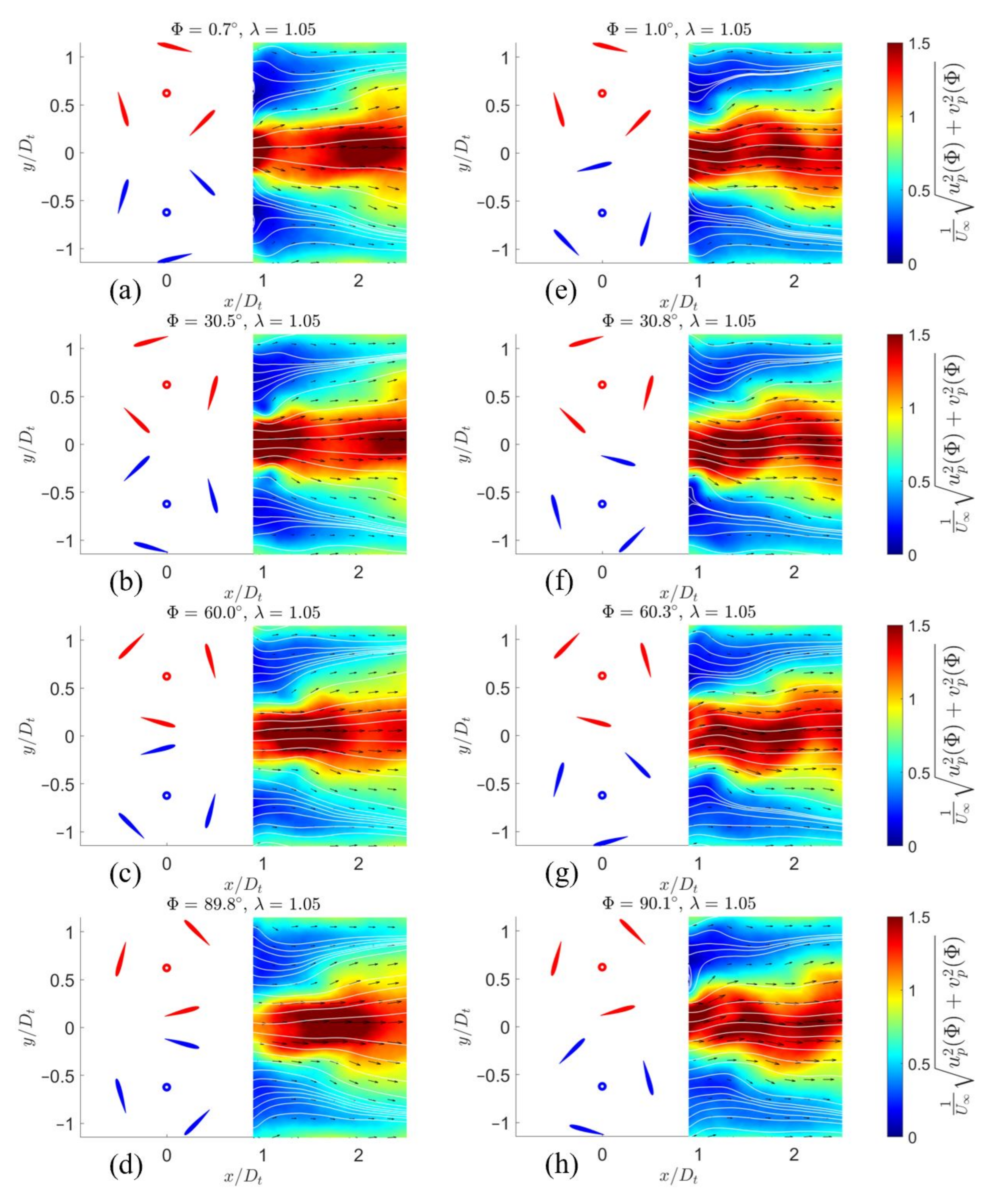
3.1. Effect of Phase Difference

To observe the effect of the phase difference Δ Φ between the two turbines, the separation distance was fixed at 1.25 D t and the flow structures were captured at 4 points shown in Figure 5. For the forward and backward configurations, the chosen experimental tip-speed-ratios λ were 1.05 and 0.90, respectively, as they exhibited clear difference in the power coefficient. The power coefficient C P and tip-speed-ratio λ are defined as
C P = T H ω ¯ 1 2 ρ A U 3 ,
λ = ω R t U
where T H is the hydrodynamic torque exerted on the turbine, ω is the turbine rotating speed, ρ is the water density, A is the system frontal area, R t is the turbine radius, and U is the reference inlet velocity. The frontal area A was defined as 2 D t h for the twin turbine configurations, where D t is the rotor diameter and h is the height that the blades were submersed in water.
In terms of the forward counter-rotating configurations (Figure 4a,b), the 60 ° phase difference was observed to break the symmetry of the near-wake. Figure 6 shows the flow structure of the two configurations at the tip-speed-ratio of 1.05 and approximately the same turbine angles. For the case of Δ Φ = 0 ° , the streamlines stayed relatively flat for the whole phase from 0 ° to 120 ° , except for Figure 6a and Figure 7, when two re-circulation zones were formed behind the turbines. On the other hand, obvious fluctuations of the flow can be seen in Figure 6e–h. Besides the fast flow zone in the middle oscillating up and down, the re-circulation zone behind the turbines also alternatively appeared in Figure 6f, behind turbine T2 in blue color, and in Figure 6h and Figure 8, behind turbine T1 in red color.
Similar behavior was captured for the backward counter-rotating configurations at Δ Φ = 0 ° and Δ Φ = 60 ° . Small parts of the re-circulation zones behind the turbine could be seen simultaneously in Figure 9c around x / D t < 1 for Δ Φ = 0 ° . The wake symmetry was also broken for Δ Φ = 60 ° with the meandering streamlines. Additionally, the re-circulation zones were created alternatively behind turbine T2 in blue color, in Figure 9e and Figure 10, and turbine T1 in red color, in Figure 9g.
Results of the four operating points in this sub-section indicate that imposing a phase angle difference between the turbine would break the symmetry of the near-wake structure, create more flow fluctuations and kinetic energy in the near-wake compared to 0 ° phase difference, and therefore decrease the system power output.

3.2. Effect of Separation Distance

The effect of the separation distance between the turbines can be examined by analyzing the counter-rotating at Δ Φ = 60 ° and overlapping configurations. Figure 11 shows the four measurement points used for this examination. The points were chosen for the same reason of obviously distinguishable power coefficient values, as in the previous sub-section.
At the same phase difference of Δ Φ = 60 ° and different separation distances, moving the turbines closer to each other suppressed the fast flow zone, which was the source of kinetic energy loss (Figure 12). Furthermore, no re-circulation zone was observed for the forward overlapping case in Figure 12e–h, while part of a re-circulation zone was seen behind turbine T2, in blue color, in Figure 12a and behind turbine T1, in red color, in Figure 12d.
Regarding the backward counter-rotating and overlapping configurations, strongly skewed streamlines were observed for both cases at λ = 0.75 (Figure 13). Decreasing the distance between the turbines simply reduced the area of the slow zone in the wake. Re-circulating flows can be seen on all of the plots in Figure 13. These operating points were on the low power output side of the power curves, which suggested that turbine geometry should be designed to avoid re-circulation if possible.

3.3. Note on Effect of Relative Incoming Flow Angle

This experiment had limited capability in changing the relative incoming flow angle as only two different incoming angle cases were performed (forward and backward). While the forward and backward configurations created completely different flow dynamics, none of the turbine was operating inside the other’s wake. Although different turbine rotating speed created different details in the wake, Figure 6, Figure 7, Figure 8 and Figure 9 and Figure 12 and Figure 13 show qualitatively similar structures of the by-pass flow for each configuration. The water channel walls, which were located at approximately y / D t = ± 2.0 and not shown in any figures, might play important role since hydrodynamic interaction between a turbine and the experimental tunnel walls is a widely known effect. In the limited view of the PIV window, forward configurations seemed to reduce the by-pass flow velocity and kinetic energy loss and therefore produced higher power compared to the backward configurations at the same tip-speed-ratio.

3.4. Quantitative Assessment

The qualitative observation of these counter-rotating configurations shows similar tendency as the observation of the single turbine configurations discussed in Part–I so the same hypothesis was expected. The less energetic flow field is observed behind the turbines, the more turbine power output is expected. Part–I suggested that the output energy could be evaluated by taking the average of the fluid kinetic energy over space and time. The time averaged kinetic energy of the cases shown in Figure 6, Figure 7, Figure 8, Figure 9, Figure 10, Figure 11, Figure 12 and Figure 13 can be seen in Figure 14. The recorded velocity fields were time-averaged as u ¯ and v ¯ and the non-dimensionalized time-averaged kinetic energy is defined as
K ¯ = 1 2 ( u ¯ 2 + v ¯ 2 ) 1 U 2 ,
which can be used to evaluate the average kinetic energy over the line x / D t = 1.0 as
P K ¯ ( x = 1 ) = 1 | y 2 y 1 | y = y 1 y 2 K ¯ ( x = 1 , y ) d y .
As shown in Table 1, this representative parameter of the averaged kinetic energy has an inversely proportional relationship with the power coefficient for all the cases discussed in Figure 6, Figure 7, Figure 8, Figure 9, Figure 10, Figure 11, Figure 12 and Figure 13. The tendency of the fluid kinetic energy in the near-wakes of the counter-rotating configurations was concluded to be qualitative and quantitative similar to a single turbine.

4. Conclusions

This article presented experimental fluid flow results of the near wake region of two independent marine hydrokinetic turbines in six different counter-rotating configurations. A 2D particle image velocimetry method was applied to capture the phase-averaged flow fields right behind the turbines. By comparing the configurations at the same tip-speed-ratios, effects of varying the turbine separation distance, phase angle difference, and relative incoming flow direction could be observed.
Similar to results from Part–I with single turbines, twin turbine configurations that created strongly skewed flow streamlines and fluctuations produced less power output. Specifically, a phase difference of 60 ° broke the wake symmetry and created meandering flow fields compared to 0 ° phase angle difference. Decreasing the turbine separation distance from 1.25 D t to 1.00 D t in the forward configurations suppressed the high kinetic energy flow in the middle area and thus produced more power. On the other hand, reducing the separation distance for the backward configurations only decreased the slow zone in the near-wake while keeping the general structures similar to each other. Lastly, switching from the forward to backward configurations largely affect the by-pass flow which could be attributed to the interaction with the channel walls. The authors hope to address this wall interaction question in future experimental and numerical work.
Other than showing the effect of different counter-rotating configurations of a twin turbine system, the flow measurement results can also be used to validate future numerical models. In the spirit of open-access work, this article is accompanied by full numeric data of the flow fields which can be freely downloaded from [18].

Author Contributions

Conceptualization, M.N.D. and S.O.; methodology, M.N.D.; software, M.N.D.; validation, M.N.D.; formal analysis, M.N.D. and T.K.; investigation, M.N.D. and T.K.; resources, S.O.; data curation, M.N.D.; writing—original draft preparation, M.N.D. and S.O.; writing—review and editing, S.O.; visualization, M.N.D.; supervision, T.K. and S.O.; project administration, S.O.; funding acquisition, S.O. All authors have read and agreed to the published version of the manuscript.

Funding

This research received no external funding.

Institutional Review Board Statement

Not applicable.

Informed Consent Statement

Not applicable.

Data Availability Statement

The data presented in this study are openly available in Kaggle at doi: 10.34740/kaggle/dsv/2279541, reference number 2279541.

Acknowledgments

M.N.D. thanks Koji Fukagata, Keita Ando, Ivan Alayeto, Kana Kumazawa, Claudio Padricelli, Uros Markovic, Naomichi Baba, Naoya Sumimura, Julio Barros, Anna Mizobuchi, Mehdi Badri, and Laura Beninati for fruitful discussions and help with the experimental setup. M.N.D. also highly appreciates Sao Cao Bu Le, Nam Pho Hoang, and Saruzy Be De Nguyen for their help in improving Minh’s computer skill. The authors also thank Hisae Mizuno for her endless help with the grant and logistics paperwork. This research was partly supported by the Keio Design The Future award and the Keio Leading-Edge Laboratory of Science and Technology Grant.

Conflicts of Interest

The authors declare no conflict of interest.

Abbreviations

The following abbreviations are used in this manuscript:
MHKMarine hydrokinetic turbine
VAWTVertical axis wind turbine
PIVParticle image velocimetry

References

  1. Dabiri, J. Potential order-of-magnitude enhancement of wind farm power density via counter-rotating vertical-axis wind turbine arrays. J. Renew. Sustain. Energy 2011, 3, 043104. [Google Scholar] [CrossRef] [Green Version]
  2. Brownstein, I.D.; Wei, N.J.; Dabiri, J.O. Aerodynamically Interacting Vertical-Axis Wind Turbines: Performance Enhancement and Three-Dimensional Flow. Energies 2019, 12, 2427. [Google Scholar] [CrossRef] [Green Version]
  3. Jiang, Y.; Zhao, P.; Stoesser, T.; Wang, K.; Zhou, L. Experimental and numerical investigation of twin vertical axis wind turbines with a deflector. Energy Convers. Manag. 2020, 209, 112588. [Google Scholar] [CrossRef]
  4. Li, Y.; Calisal, S. Modeling of twin-turbine systems with vertical axis tidal current turbines: Part 1—Power Output. Ocean Eng. 2010, 37, 627–637. [Google Scholar] [CrossRef]
  5. Li, Y.; Calisal, S. Modeling of twin-turbine systems with vertical axis tidal current turbine: Part 2—Torque Fluctuation. Ocean Eng. 2011, 38, 550–558. [Google Scholar] [CrossRef]
  6. Bachant, P.; Wosnik, M.; Gunawan, B.; Neary, V. Experimental study of a reference model vertical-axis cross-flow turbine. PLoS ONE 2016, 11, e0163799. [Google Scholar] [CrossRef] [PubMed] [Green Version]
  7. Bachant, P.; Wosnik, M. Performance measurements of cylindrical- and spherical-helical cross-flow marine hydrokinetic turbines, with estimates of exergy efficiency. Renew. Energy 2014, 74, 318–325. [Google Scholar] [CrossRef]
  8. Ross, H.; Polagye, B. An experimental assessment of analytical blockage corrections for turbines. Renew. Energy 2020, 152, 1328–1341. [Google Scholar] [CrossRef] [Green Version]
  9. Araya, D.; Colonius, T.; Dabiri, J. Transition to Bluff-Body Dynamics in the Wake of Vertical-Axis Wind Turbines. J. Fluid Mech. 2017, 813, 346–381. [Google Scholar] [CrossRef] [Green Version]
  10. Doan, M.; Kai, Y.; Obi, S. Twin Marine Hydrokinetic Cross-Flow Turbines in Counter Rotating Configurations: A Laboratory-Scaled Apparatus for Power Measurement. J. Mar. Sci. Eng. 2020, 8, 918. [Google Scholar] [CrossRef]
  11. Doan, M.; Kai, Y.; Takuya, K.; Obi, S. Flow Field Measurement of Laboratory-Scaled Cross-Flow Hydrokinetic Turbines: Part 1—The Near-Wake of a Single Turbine. J. Mar. Sci. Eng. 2021, 9, 489. [Google Scholar] [CrossRef]
  12. Araya, D.; Dabiri, O. A comparison of wake measurements in motor-driven and flow-driven turbine experiments. Exp. Fluids 2015, 56, 150. [Google Scholar] [CrossRef]
  13. Suryadi, A.; Ishii, T.; Obi, S. Stereo PIV measurement of a finite, flapping rigid plate in hovering condition. Exp. Fluids 2010, 49, 447–460. [Google Scholar] [CrossRef]
  14. Suryadi, A. The Phase-Avreaged Velocity Measurement and the Estimation of Pressure Force of a Periodically Moving Body. Ph.D. Thesis, Keio University, Yokohama, Japan, 2011. [Google Scholar]
  15. Doan, M.N.; Alayeto, I.H.; Kumazawa, K.; Obi, S. Computational fluid dynamic analysis of a marine hydrokinetic crossflow turbine in low Reynolds number flow. In Proceedings of the ASME-JSME-KSME 2019 8th Joint Fluids Engineering Conference, San Francisco, CA, USA, 28 July–1 August 2019; Volume 2, p. V002T02A067. [Google Scholar]
  16. Antonia, R.; Bisset, D.; Browne, L. Effect of Reynolds number on the topology of the organized motion in a turbulent boundary layer. J. Fluid Mech. 1990, 213, 267–286. [Google Scholar] [CrossRef]
  17. Kim, H.; Kline, S.; Reynolds, W. The production of turbulence near a smooth wall in a turbulent boundary layer. J. Fluid Mech. 1971, 15, 133–160. [Google Scholar] [CrossRef]
  18. Doan, M. PIV Counter Rotating Turbines; Kaggle: San Francisco, CA, USA, 2021. [Google Scholar] [CrossRef]
Figure 1. An illustration of the twin turbine apparatus variations: (a) counter-rotating and (b) overlapping turbines with the separation distance of 1.25 D t and 1.00 D t . The figure was adapted from [10].
Jmse 09 00777 g001
Figure 2. An overview of the monoscopic particle image velocimetry setup. The figure was adapted from [11].
Jmse 09 00777 g002
Figure 3. An example of the PIV calculation points on a raw picture.
Jmse 09 00777 g003
Figure 4. Different turbine configurations used in the near-wake measurement experiments: (a) forward counter-rotating at Δ Φ = 0 ° , (b) forward counter-rotating at Δ Φ = 60 ° , (c) forward overlapping at Δ Φ = 60 ° , (d) backward counter-rotating at Δ Φ = 0 ° , (e) backward counter-rotating at Δ Φ = 60 ° , and (f) backward overlapping at Δ Φ = 60 ° . The red and blue circles illustrate the turbine T1 and T2 rotational center correspondingly. The flow measurement areas are enclosed inside the black dashed lines.
Jmse 09 00777 g004
Figure 5. The power curves of counter-rotating configurations, which was adapted from [10], with the flow measurement points highlighted.
Jmse 09 00777 g005
Figure 6. The phase-averaged flow fields behind the forward counter-rotating configurations at λ = 1.05 . The power coefficients of these configurations are 0.116 and 0.103 for Δ Φ = 0 ° (ad) and Δ Φ = 60 ° (eh) correspondingly. The displayed phase angles Φ belong to turbine T1 in red color. The color shows the non-dimensionalized phase-averaged velocity magnitude.
Jmse 09 00777 g006
Figure 7. A zoomed in picture of Figure 6a. The re-circulation zones behind the turbines are enclosed in the purple solid lines.
Jmse 09 00777 g007
Figure 8. A zoomed in picture of Figure 6h. The re-circulation zone behind turbine T1 is enclosed in the purple solid lines.
Jmse 09 00777 g008
Figure 9. The phase-averaged flow fields behind the backward counter-rotating configurations at λ = 0.90 . The power coefficients of these configurations are 0.108 and 0.103 for Δ Φ = 0 ° (ad) and Δ Φ = 60 ° (eh) correspondingly. The displayed phase angles Φ belong to turbine T1 in red color. The color shows the non-dimensionalized phase-averaged velocity magnitude.
Jmse 09 00777 g009
Figure 10. A zoomed in picture of Figure 9e. The re-circulation zone behind turbine T2 is enclosed in the purple solid lines.
Jmse 09 00777 g010
Figure 11. The power curves of counter-rotating and overlapping configurations at Δ Φ = 60 ° , which was adapted from [10], with the flow measurement points highlighted.
Jmse 09 00777 g011
Figure 12. The phase-averaged flow fields behind the forward counter-rotating (ad) and overlapping (eh) configurations at Δ Φ = 60 ° and λ = 0.95 . The power coefficients of these configurations are 0.120 and 0.128 for forward counter-rotating ( Δ Φ = 60 ° ) and overlapping configuration correspondingly. The displayed phase angles Φ belong to turbine T1 in red color. The color shows the non-dimensionalized phase-averaged velocity magnitude.
Jmse 09 00777 g012
Figure 13. The phase-averaged flow fields behind the backward counter-rotating (ad) and overlapping (eh) configurations at Δ Φ = 60 ° and λ = 0.75 . The power coefficients of these configurations are 0.097 and 0.092 for forward counter-rotating ( Δ Φ = 60 ° ) and overlapping configuration correspondingly. The displayed phase angles Φ belong to turbine T1 in red color. The color shows the non-dimensionalized phase-averaged velocity magnitude.
Jmse 09 00777 g013
Figure 14. The time-averaged kinetic energy of the near-wakes for the cases shown in Figure 6, Figure 7, Figure 8, Figure 9, Figure 10, Figure 11, Figure 12 and Figure 13.
Jmse 09 00777 g014
Table 1. Comparison of each configuration’s temporally and spatially averaged kinetic energy at x / D t = 1.0 and the associated power coefficient.
Forward/Backward λ Δ Φ Separation Distance C P P K ¯ ( x = 1 )
Forward1.0501.250.1160.263
Forward1.05 60 ° 1.250.1030.268
Backward0.9001.250.1080.259
Backward0.90 60 ° 1.250.1030.264
Forward0.95 60 ° 1.250.1200.277
Forward0.95 60 ° 1.000.1280.227
Backward0.75 60 ° 1.250.0970.269
Backward0.75 60 ° 1.000.0920.357
Publisher’s Note: MDPI stays neutral with regard to jurisdictional claims in published maps and institutional affiliations.

