Article

Application of Large Eddy Simulation to Predict Underwater Noise of Marine Propulsors. Part 1: Cavitation Dynamics

1
SCHOTTEL GmbH, Schottelstr. 1, 56281 Dörth, Germany
2
Institute for Fluid Dynamics and Ship Theory (FDS), University of Technology (TUHH), Am Schwarzenberg-Campus 4(C), 21073 Hamburg, Germany
*
Author to whom correspondence should be addressed.
J. Mar. Sci. Eng. 2021, 9(8), 792; https://0-doi-org.brum.beds.ac.uk/10.3390/jmse9080792
Submission received: 7 June 2021 / Accepted: 26 June 2021 / Published: 22 July 2021

Abstract

:
Marine propulsors are identified as the main contributor to a vessel’s underwater radiated noise as a result of tonal propeller noise and broadband emissions caused by its induced cavitation. To reduce a vessel’s signature, spectral limits are set for the propulsion industry, which can be experimentally obtained for a complete vessel at the full-scale; however, the prediction capability of the sound sources is still rudimentary at best. To adhere to the regulatory demands, more accurate numerical methods for combined turbulence and two-phase modeling for a high-quality prediction of acoustic sources of a propeller are required. Several studies have suggested implicit LES as a capable tool for propeller cavitation simulation. In the presented study, the main objective was the evaluation of the tip and hub vortex cavitating flows with implicit LES focusing on probable sound source representation. Cavitation structures for free-running propeller test cases were compared with experimental measurements. To resolve the structure of the tip vortex accurately, a priory mesh refinement was employed during the simulation in regions of high vorticity. Good visual agreement with the experiments and a fundamental investigation of the tip cavity structure confirmed the capability of the implicit LES for resolving detailed turbulent flow and cavitation structures for free-running propellers.

1. Introduction

The marine propeller has been identified as a primary source of underwater radiated noise [1,2], with tonal peaks at distinct blade passing frequencies, and its induced cavitation, generating broadband noise emissions. Regulatory institutions are beginning to implement requirements set by classification societies [3], which need to be confirmed before the vessel’s existence. However, the exact underlying physical mechanisms of noise generation due to large-scale cavitation structures and its dynamic evolution are poorly understood. In order to reduce propeller noise emissions as part of a vessel’s underwater noise spectrum, the prediction methods are first required to reach sufficiently high accuracy over the complete frequency range of interest.

1.1. State of the Art

When designing a high-performance marine propeller for high-area loads and low cavitation numbers, there is always a tradeoff between efficiency and risk of cavitation, which is known to have detrimental effects that might be experienced as a loss of thrust or material erosion, and which are usually accompanied by the generation of broadband noise as a result of dynamic cavitation structures and single bubble collapses of varying diameter. The exact topology and shape, as well as dynamic behavior, of the cavitation structures depend highly on the specific propeller design, its inflow, and operation point.
A modern propeller is designed to avoid harmful cavitation types; however, tip- and hub-vortex cavitation themselves are, in most cases, not erosive for the propeller itself and can, depending on the installation situation, be acceptable in favor of higher efficiency, which typically make these the primary contributors to acoustic volume sources at the propeller and in its slipstream [4] above cavitation inception vessel speeds and, thus, the most important to understand. Due to the coherent structure and stability of these types of cavitation, it can be expected that a Eulerian finite volume method with a volume-of-fluid (VOF) phase modeling approach without consideration of single bubble contributions is sufficient to predict the noise generation, under the assumption that the turbulence-cavitation interaction on the blade and in the propeller slipstream is sufficiently resolved. Even though an energy cascade for the process of cavitation from macrostructures, i.e., what can be simulated with VOF, to the dynamics of smaller scales has been proposed, the premise of this study is that modeling large-scale cavities is sufficient for the noise prediction as, physically, a synchronized implosion of microbubbles is hypothesized [5] and assumed to occur at the combined closure part and cavity wake region of a stable sheet cavity [6].
While studies on hydrofoils’ flows have found little dependence of the cavitating tip vortex trajectory on physical parameters [7], it is inherently connected to the tip vortex of a propeller, which evolves in the propeller slipstream and, in itself, is unstable after a certain running length [8]. Typically induced by a sheet cavity forming at the suction side leading edge of the propeller, which is accompanied by a roll-up process due to the pressure gradient, upon leaving the blade surface, the tip vortex formation evolves initially over a mixing zone. During the disintegration process of the sheet cavity, the remaining structures dissolve or migrate into the cavitating tip vortex. It is proposed that the transition processes in the mixing zone fundamentally determine the geometric properties of the cavitating tip vortex as a deformable surface carrying acoustic waves and, as a result, generate one of the modes of a vibrating hollow core vortex from Figure 1 [9,10]. As the tip vortex itself is a relatively stable flow structure and contributes only with periodic displacement in the blade passing frequency, it is hypothesized that the higher-frequency acoustic emissions originate in these overlaying vibrations and additionally collapse from individual detached bubbles. Experimentally, it is still difficult to exactly identify the topology and shape of the tip vortex cavity until methods for the documentation of three-dimensional surfaces belonging to the phase interface are widely utilizable, as there are often secondary effects impeding the visual analysis. Thus, numerical methods have the potential to increase the understanding of the underlying mechanisms of tip vortex cavity formation and possibly associated noise generation.
The complex problem of underwater radiated noise, emitted by a propeller and its induced cavitation, therefore, requires the study of the three fundamental physical phenomena:
  • Turbulence;
  • Two-phase flow;
  • Noise source description and propagation.
While it is advantageous to decouple the latter in the case of underwater acoustics to utilize the incompressibility assumption of the medium in the hydrodynamic part of the simulation, the first two are closely connected and interdependent.
Typically, the finite volume method is used for the hydrodynamic aspect of the simulations, with the most common turbulence modeling approach based on ensemble averaging of turbulent fluctuations in the flow, taking advantage of the statistical properties of turbulence with the Reynolds-averaged Navier–Stokes (RANS) equations. With adequately refined meshes and small time steps, a detailed propeller tip-vortex flow can be resolved for propeller free-running cases at the model- and full-scale, demonstrating scale effects regarding tip-vortex behavior [11]. However, it is expected that for noise prediction, this type of turbulence averaging affects the results for higher-frequency sound pressure. Recent studies comparing the tip vortex flow of a hydrofoil [12] have highlighted the requirement to resolve at least large and medium turbulent length scales, which comes with a significant computational cost in the form of large eddy simulation approaches. Hybrid turbulence modeling methods are increasing the feasibility of realizing such a requirement with acceptable numerical effort for research applications as studies with detached eddy simulation (DES) [13] and delayed DES [14], which lead to an excellent reproduction of cavitation features for marine propellers, have shown with the PPTC’11 case. The Newcastle propeller round robin test case in condition C2 [15], which was also the subject of this study, was simulated with DES, leading to good agreement with the cavitation observations [16]. An alternative with theoretically less computational resource requirements was identified in the implicit large eddy simulation (ILES) method for marine propellers, as no additional turbulence transport equations and no subgrid-scale model have to be solved [17]. The noise propagation of a propeller was validated with the Newcastle or R/V Princess Royal test case [18], including the ship hull with ILES. With a solver that considers compressibility effects, different turbulence modeling approaches for specific Reynolds number regimes were investigated [19] and, from the good agreement of the cavity structures with the respective experimental observations, it was found that the model itself has little influence, although it seemed that hybrid models produce a greater level of detail of the trailing cavity structures.
To avoid numerical diffusion and maintain the cavitating tip vortex in the propeller slipstream, a high mesh resolution is necessary; however, sufficient refinement downstream of the propeller is not feasible with manageable resource demand. This is why smart refinement strategies are required, which was demonstrated for RANS investigations of a hydrofoil and a propeller, where a priory mesh refinement and an adaptive mesh refinement (AMR) were compared. Different criteria for the resolution of cavitating vortices are available in the literature [20], from 16 cells across the vortex, based on numerical studies [12] over recommendations based on globally or locally unstable flows [21] or analytical derivations based on the inertial subrange length [13] to experimental observations [22]. In another study of the Newcastle case, an AMR strategy based on the pressure distribution was successfully utilized to maintain the cavitating tip vortex in the propeller slipstream with a rudder [23]. The AMR method was particularly important and likewise challenging, when cavitating trailing vortices were interacting with a non-axisymmetric structural obstacle such as a rudder downstream of the propeller, where the vortices break up and sound sources are presumably located, making this an important future research topic.

1.2. Contributions of Current Work

The acoustic evaluation of a marine propeller with CFD methods requires accurate representation of turbulence and cavitation, which are the main sources emitting broadband and high-frequency noise, whereas the water volume displacement by the blades creates only a distinct tonal noise at multiples of the blade passing frequency. The latter can also be predicted by low-fidelity methods with sufficient accuracy; however, the broadband noise sources require high spatial and temporal resolution of flow features, which necessitates resolving low- and medium-wavelength turbulence with LES. In this work, an industry-oriented feasibility study of an ILES-based numerical evaluation was executed, by analyzing the turbulence structure in the propeller slipstream, which, in particular, entails the cavitating trailing vortices. A detailed look at the ability of finite volume-based numerical simulations with a VOF Euler-based approach and a priory mesh refinement to capture vapor structures and its interaction with turbulence was taken. The exact underlying mechanisms of noise generation due to different cavitation structures in the propeller slipstream, particularly shear and vortex cavitation, are still not thoroughly understood, and it is unclear whether a VOF-based approach is able to capture the majority of noise sources, as single bubble contributions are neglected. The current study sheds light on the capabilities of this method to accurately capture cavitation macrostructures, within the margins of feasible mesh refinements with respect to numerical resources.

2. Methods

In this section, the underlying models for hydrodynamic flow calculations and treatment of the two-phase flow mixture are provided. The mathematical descriptions of Section 2.1 are based on the models implemented in the utilized OpenFOAM distribution, which is detailed in Section 2.2, together with the numerical setups for this study.

2.1. Methodology

2.1.1. Resolving Turbulence

Based on successful studies regarding cavitating tip-vortex marine propeller flow with ILES [17] and its theoretically superior use of calculation resources, as well as its inherent simplicity, this approach is promising for underwater radiated noise predictions in a time- and resource-constricted industry environment. The simulations therefore apply implicit subgrid-scale modeling without specific wall treatment models, which imposes an appropriate space-time resolution to capture the characteristic scales inherent to the system’s evolution. The assumption of the implicit approach is that the numerical dissipation of the convective term is of the same order of magnitude as the subgrid stress tensor and can influence the resolved scales in a similar manner as a subgrid-scale model. Thus, the conservation equations for a transient incompressible homogeneous mixture m , with low-pass-filtered quantities denoted with an overbar, are
ρ m t + ρ m u ¯ i x i = 0 ,
( ρ m u ¯ i ) t + ρ m u ¯ i u ¯ j x i = p ¯ x i + x j S ¯ i j B i j + ρ m g i ,
where the viscous stress tensor is S i j = μ u i x j + u j x i , based on the deformation rate tensor. In the case of a water-vapor mixture, only one species transport equation and a phase fraction transport equation are necessary. Ideally, a dissipative velocity divergence scheme discretization is combined with this approach, such as the linear-upwind stabilized transport scheme. While this approach promises good agreement with the high wavenumber turbulent fluctuation damping, the stability for cavitating propeller tip vortex flows was found to not be sufficient for extended acoustic calculations, resulting in the utilization of a standard limited second-order central differencing scheme. In our previous studies [20,24,25], the superior qualities regarding the resolution of tip and hub vortex details were confirmed, for instance, in hydrofoil test cases. While the PISO solution algorithm was initially selected for its speed, later investigation resulted in an improved prediction of forces with the PIMPLE algorithm at a minimum of three outer corrector loops and three internal pressure corrector loops.

2.1.2. Two-Phase Flow

For phase transition, a homogeneous mixture model was applied, where a source term is introduced to the mixture transport equations S m = ρ l ρ v ρ l S α and an additional liquid phase fraction transport equation is solved:
α t + · α u + · u c α 1 α = S α ,
where u c is the artificial compression velocity field activated at the interface. Among others, the Schnerr–Sauer cavitation model, which is derived from the Rayleigh–Plesset equation, was selected for its robustness and independence of any empirical parameters. The model is based on simplifications that do not consider:
  • Viscous effects;
  • Nonspherical bubble shape;
  • Interface surface tension and sliding interfaces;
  • Bubble interactions;
  • Compressibility.
The mass transfer rate depends on the local pressure p and the saturation pressure p V :
m ˙ + = C V 1 + α N u c α 3 ρ L ρ V ρ R 2 3 ρ L 1 p p V min p p V , 0 ,
m ˙ = C c α 3 ρ L ρ V ρ R 2 3 ρ L 1 p p V max p p V , 0 ,
where C V is the vaporization and C C is the condensation coefficient, which were set to unity in this study. The bubble radius is
R =   3 1 + α N u c α 4 π n 0 α 3
and depends on the nucleation volume fraction,
α N u c = V N u c 1 + V N u c
with the nucleation volume of V N u c = π n 0 d N u c 3 6 , where the parameters for the model are the nuclei density n 0 and the initial nuclei diameter d N u c , which were set to the constant values. The given values in Table 1 led to stable calculations and good details on the cavity surfaces [20].

2.2. Numerical Setup

All investigations were executed with the open-source code OpenFOAM written in C++, which utilizes a cell-centered collocated finite volume method for spatial discretization. The distributions used in this study were from Engys Ltd. and involved HELYX versions 3.1.1 to 3.2.0. The applied interPhaseChangeDyMFoam solver with dynamic mesh functionality has the capability to solve for two incompressible, isothermal immiscible fluids with a VOF interface employing phase-change calculations with the above-specified Schnerr–Sauer cavitation model. The focus is on two model propeller test cases with extensive experimental documentation used to develop methods for the analysis of propeller underwater radiated noise, namely the PPTC’11 [26] and the Newcastle propeller round robin benchmark test case [15]. These analyses were intended to verify the applicability of the proposed approach for the simulation of cavitating trailing vortices with regard to resolving the turbulence and phase transition adequately to provide the information base for subsequent analysis of underwater noise prediction capabilities. A full model of a propeller instead of a sector model was calculated with sliding mesh interfaces for the following reasons:
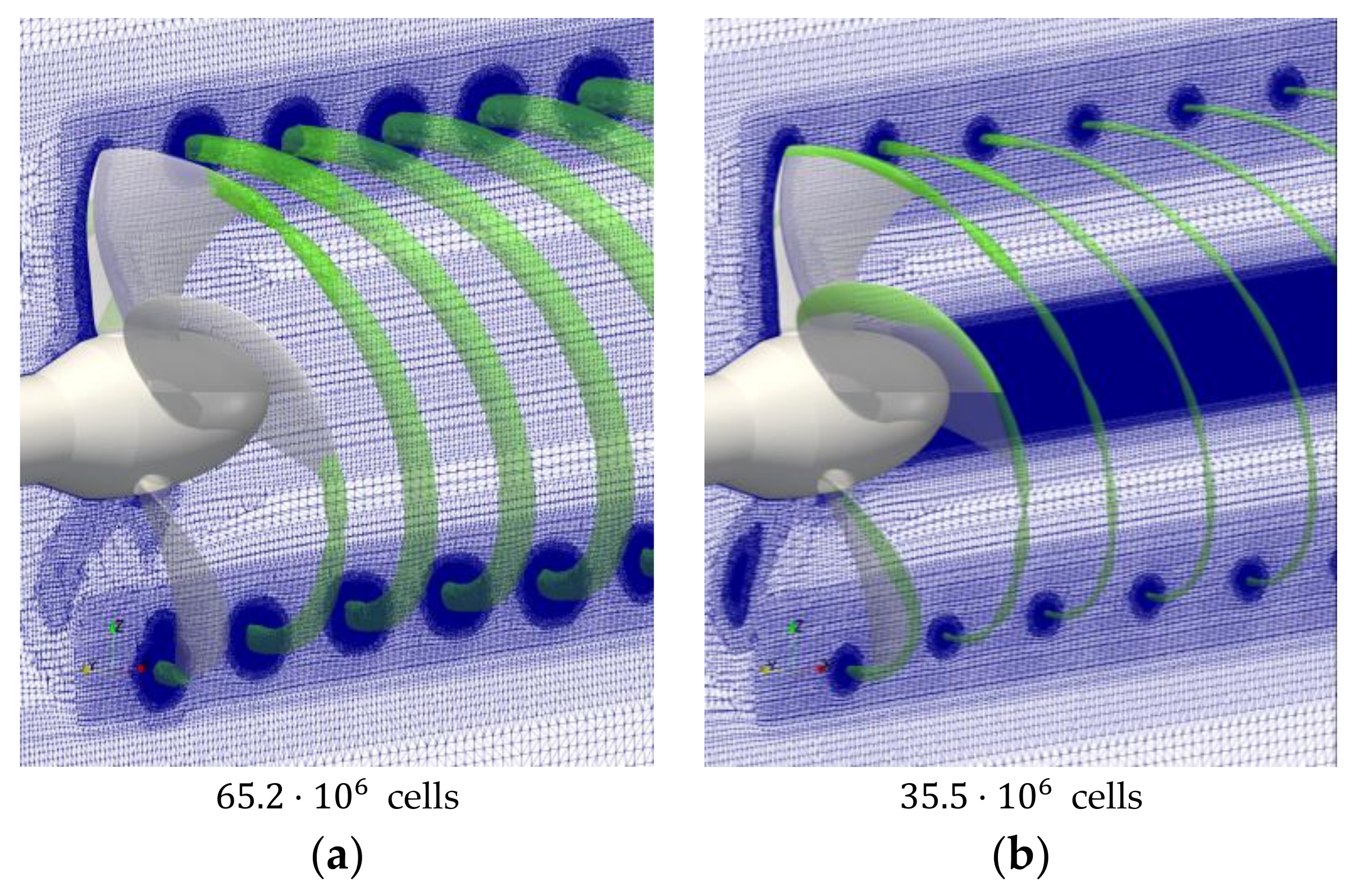
  • To ensure that non-axisymmetric turbulence and cavity structures at the symmetry axis are resolved;
  • In subsequent behind-ship condition setups, the non-axisymmetric inflow caused by the ship wakefield or inclined shaft lines and possible structural obstacles in the propeller slipstream, such as rudders or azimuthing propulsor housings, have to be considered.
The flow of the PPTC’11 propeller was investigated in push configuration, with a propeller diameter of D M = 0.25 m for condition 2.3.1 with J = 1.019 , n = 25 Hz, and σ n = 2.024 . The main focus lies in the prediction of the features of the steady cavitating tip and a developed hub vortex, which is ideal for the development of methods for the detailed analysis of trailing turbulence and phase-change phenomena. The Newcastle propeller test case in round robin conditions C1 to C3 and C6 [27], as summarized in Table 2, with the University of Genoa (UNIGE) test setup and D M = 0.22 m experiences tip vortex cavitation to a varying extent in the pull configuration and features acoustic spectral measurements by six different experimental test facilities for the analysis of acoustic sources and propagation. Geometric data of the PPTC’11 and Newcastle propeller from the round robin test are readily available.
The fundamental mechanisms for the generation of turbulent fluctuations are either based on shear in the boundary layer at the wall or by flow shear behind sharp edges of solid bodies, such as the trailing edges of propellers. As the tip vortex flow arises primarily by the latter, the followed approach relaxes the strict wall modeling associated with LES in favor of reduced numerical effort, which is of particular importance for acoustic simulations, where fine time steps and a high number of rotations are essential for spectral analyses. While the law of the wall demands a high degree of near-wall mesh resolution for LES, for which several suggestions are found in the literature, such as y + 2 , as well as x + 10 and z + 5 [28], where y is the wall orthogonal coordinate axis and x indicates the streamwise direction, it is considered infeasible for industry use due to the highly inflated cell count and the corresponding numerical resource requirements. The precursor RANS step, on the other hand, necessitates either y + 1 for low Reynolds wall treatment or y + 30 values for high Reynolds wall modeling. The initial mesh for the PPTC’11 case features y + 1 except near the trailing edge, and the mesh is illustrated in Figure 2a, where additional refinements along the shaft and the tunnel walls of the experiment’s cavitation tunnel are also visible. For the Newcastle case in (b), a higher and, thus, more unfavorable y + 10 wall distance of the first cell on the propeller blades was achieved. This might affect the prediction of forces negatively as no wall model is utilized in the LES part of the simulation, while the RANS is expected to show higher deviations regarding integral values due to the wall model’s reduced accuracy in the buffer layer, even though a proprietary “all y + wall treatment” wall model is utilized in the simulations without cavitation. It is useful to find out whether the tip vortex cavitation dynamics are affected by the reduced wall resolution.
The meshing consists of two phases: the initial mesh with which the simulation is started and, once the initial simulation is converged, a manually employed a priory mesh refinement. The initial meshes already consider the expected cavitation area on the blade surface with a distance refinement on the suction side near the leading edges and the cavitating tip vortex regions with an annulus refinement from r R 0.68 to r R 1.10 with an axial extent of 2 D from the propeller plane. An additional refinement downstream of the blade tips is incorporated in the Newcastle case, as the tip vortex strength is considerably lower than the PPTC’11 case. Both cases differ in the configuration of the propeller shaft, where each shaft line is extruded toward the next domain face intersection to reduce interaction effects, which avoids any hub vortex in the Newcastle case. In the figures, the green dashed lines indicate the sliding mesh interface and, thus, the extent of the rotating region, which features an increased refinement level compared to the surrounding mesh.
All simulations shared an identical base setup with a velocity inlet, depending on the advance ratio and a constant pressure outlet set to the environment pressure, meaning that pressure is independent of the gravity direction vector, which, in model-scale, is a sufficiently close approximation of the experimental conditions, and the remaining surfaces are defined as walls. The rotating region is defined as a cyclic arbitrary mesh interface (AMI). The phase transition solver interPhaseChangeDyMFoam is based on the physical dynamic pressure definition, which prevents an initial steady-state calculation with other solvers, which are typically based on the kinematic pressure definition to quickly achieve flow convergence. Instead, a transient precursor RANS simulation with time steps of Δ t = 1 ° was employed, during which cavitation is suppressed by setting the saturation pressure to p s a t = 1 10 10 P a . Cavitation was subsequently activated by incrementally raising the saturation pressure to the value corresponding to the experiment’s temperature. Beginning with the activation of ILES, a reduced time step of Δ t = 0.1 ° is necessary for stability reasons, compared to the large stable RANS time step, increasing calculation effort. Note that calculation effort inflates significantly once phase transition is activated, as a result of the additional transport equation and accompanying necessary large number of corrector loops for the equations, especially regarding the α -solver. In addition, a high degree of relaxation of α was applied to support the numerical stability with active cavitation.
In each simulation step, convergence is checked by monitoring the forces and moments of the propeller, as numerical equation residuals might converge prior to the integral values, especially for transient calculations. To allow for an investigation over time with videos, at least two more rotations are calculated afterward, which are used to visually confirm convergence of the trailing vortex structures similarly to the images in Table 3 or Table 4, as the integral propeller values, in turn, converge before the slipstream flow structures. In the cavitating simulations, a visual observation of the α 0.5 isosurfaces over time was conducted and the evolution of its surface area was monitored to determine convergence of the solution in addition to the previous measures. With the described monitoring, the RANS calculations were run for around 12 full rotations, which themselves were started from a potential flow initialization, before the solver was switched to ILES, which was then run for two rotations before switching on cavitation, which was gradually performed over about one rotation. Following this procedure, the cavitating part of the simulation was run for another two rotations. For the a priory mesh refinement, another three rotations were calculated after each meshing step.
Whereas in the initial RANS setup, further reduction in the time step below Δ t = 1 ° showed no significant changes in details or axial extent of the vortex structures, the time step affected the ILES results to a high degree as both the tip- and hub-vortex showed a longer axial evolution extent and greater detail on the same initial mesh, which is illustrated in Table 3. For the PPTC’11 case, the same Q-criterion isosurface extended much longer axially for the LES than for the RANS case; in fact, it passed the refined region of the mesh and the sliding interface and dissipated only in the coarse region of the mesh, due to numerical diffusion. The tip vortex details were unaffected by further reduction in the time step for ILES, while the hub vortex details appeared to fade for higher temporal resolution. This could possibly be a direct result of insufficient numerical diffusion to accurately mimic the influence of the higher-frequency unresolved turbulent length scales, due to lower flow velocity in the hub vortex region compared to the tip vortex region. While LES typically applies C F L numbers of around 1, the focus is on the propeller slipstream and its contribution to underwater noise by turbulence and trailing vortex cavitation, which is why the geometric vorticity information was used as an indication of the quality of the temporal resolution. In the table, the C F L numbers indicate the minimum and maximum numbers reached during one time step in the complete mesh. Once the a priory mesh refinement steps were employed, the highest C F L numbers were found in the trailing vortex cavitation regions, due to the extremely small cell sizes. As a result, the standard C F L criteria were relaxed to C F L < 10 in order to achieve faster convergence and, therefore, reduced calculation times. To indicate feasibility in an industry environment, the approximate numerical effort to calculate two rotations for each temporal refinement was given for both methods on 100 cores with 2.2 GHz and 64 GB of 1866 MHz DDR3 memory. Similarly, for the Newcastle case, Table 4 proves that additional temporal refinement below one third of a degree did not increase the level of detail of the trailing vortex structures in the ILES stage of the simulation.
Initial simulations confirmed that the cavitating tip vortex requires a high degree of mesh refinement to develop, for which feasible meshes regarding cell count cannot be generated with conventional meshing methods. Therefore, an a priory mesh refinement strategy based on vorticity or phase fraction is necessary for consecutive detailed investigations of the tip vortex turbulence and cavity structures. The refinement was applied at a single time step with a complete remeshing, where the source was included as a refinement surface for a distance refinement instead of an inside refinement, resulting in unnecessary large refinement diameters. This is required, as the topological space generated by the respective flow structure isosurface is not a closure. The experimentally backed minimum bubble diameter of r b = 0.1 % D P [22] is the basis for the refinement level. However, it was shown a priori that these generic criteria cannot be more than the recommendations, as it is unfeasible to resolve the complete mesh in the propeller slipstream in a sufficiently high refinement level without knowledge of the exact cavity topology and geometric positioning. As initialization for the continuation, the solution state of the last unrefined time step was adopted, from where the refinement source was also obtained.
Initially, for the PPTC’11 case, the mesh refinement was split into a two-step process, where the Q = 5 10 4 s 2 criterion is the source of an initial distance refinement to allow the tip vortex cavitation to develop, and the α = 0.5 criterion is for the second step, which is compared in Figure 3. With the reduced extent of the α 0.5 isosurface, the smaller diameter required for the refinement resulted in a highly reduced cell count and thus effective prediction of the tip vortex cavity. The tip vortex trajectory was considered grid-converged after the first step, so the high vorticity and, thus, cavitating region of the tip vortex remained in the smaller diameter refinement at all times. For the PPTC’11 case, a hub vortex refinement with a cell size identical to the tip vortex refinement was included in the second step, as the first mesh caused a considerable underprediction thereof. For the Newcastle case, only one refinement step was employed based on the higher Q = 5 10 5 s 2 value to receive a lower refinement diameter, as the α 0.5 isosurface was not available in the tip vortex region on the initial mesh, similarly to the previous case. The cell count for each refinement step for both cases is summarized in Table 5.

3. Results

In the first part, the trailing vortex analysis of the PPTC’11 and the Newcastle benchmark test case is evaluated in detail. The noncavitating tip vortex in conjunction with the propeller slipstream evolution of the Newcastle propeller with the same approach was analyzed in [20].

3.1. PPTC’11

The calculated integral values of the RANS simulation given in Table 6 agreed well with those of the experiment; however, the obtained values using the ILES differed which underlines the shortcomings of the proposed approach in calculating the integral values of the forces. As a comparison, an LES calculation with the Smagorinsky subgrid-scale model led to very good agreement regarding the forces, while the torque difference increased. The large deviations in the noncavitating part could be attributed to the missing wall model for the ILES, while the further deviations in the cavitating case may be due to differences in capturing the cavitating flow behavior on the blade seen in the experiment and the simulation. It should also be noted that the ILES for this case is run in PISO mode and improved forces are expected with a higher number of outer corrector loops, which, in turn, lead to severely increased simulation effort. The comparison LES calculation, on the other hand, applies five outer corrector loops. Interestingly, the solver pimpleDyMFoam, used here as a comparison, which is based on the kinematic pressure definition, produced more accurate results than interPhaseChangeDyMFoam, which is required to model phase change as it uses the physical pressure definition. While it is not strictly necessary to evaluate the thrust and torque coefficients anymore after the precursor RANS simulation, which is required to initialize the ILES, an inherent connection between integral forces, cavitation pattern, and noise emissions is physical and needs to be investigated.
Regarding the visual comparison of the cavitation pattern obtained by the ILES setup with the experiment shown in Figure 4, the sheet cavitation on the propeller blade was overpredicted, which is seen in most studies of this case [13]. On the initial mesh (b), the cavity isosurface, illustrated here as α = 0.5 , clearly extended beyond the tip trailing edge and formed behind the hub; however, no cavitating trailing vortices developed, due to insufficient resolution of the mesh in the respective regions. Following the first refinement step (c) based on strength of the tip vortex only, the cavity extended almost over the entire refined mesh region, showing very good agreement with the shape of the experimentally determined cavitating tip vortex regarding expansion in the propeller slipstream, which, similarly to the experiment, describes a helix-like path. In addition, the vapor core radius along its running length varied in a way that coincided with the visual evidence from the experiment, although exact matching of the findings was difficult based only on illustrative representations. In the simulation, the sheet cavity immediately turned into the vortex cavity upon leaving the blade, forming an elliptical cross-section, which turned into a circular shape along the running length of the cavity, as it overlayed with the periodically fluctuating vapor core radius along the helix-shaped running length. The mesh refinement seemed sufficient to maintain the cavitating core and the shape for a prolonged running length, as they dissolved only by entering a less refined mesh region. Introducing the second refinement step (d), there was initially a pressure interaction between the hub and tip vortex, leading to the collapse and subsequent slow reformation process of the tip vortex cavity. While the stability of the calculation was severely reduced, as a result of the high cell count in the hub vortex region and, thus, high CFL number, the interaction between hub and tip vortex cavity was emphasized by the slow convergence of both by marginally extending axially over time. Even with a reduced overall cell count compared to the first refinement step due to the different meshing strategy, the convergence was severely delayed, which somewhat challenges the proposed utilization in an industry environment. The final resulting tip vortex cavity was reduced in extent, yet the general shape coincided well with the experiment, while the hub vortex was underpredicted in cavity diameter, although it featured similar surface patterns. The reduction in the axial extent of the tip vortex cavity, when the hub vortex was resolved and the simulation settings were otherwise unchanged, confirmed the strong interaction of the pressure field between tip and hub vortex in the propeller slipstream. As convergence was extremely slow and the simulation resources were finite, a deliberate coarsening of the hub vortex region could be considered in a follow-up step, to increase stability and convergence speed.
Similar to the experiments, the discussion of complex three-dimensional shapes of unknown mathematical description, as experienced with these cavities, requires advanced methods. For a propeller shaft coinciding with the Cartesian x-axis, a helix defined by the propeller pitch angle at r x = r R 1.0 and propeller rake c , with the description
x t   =   h t + c r x cos 2 π t r x sin 2 π t ,
can be assumed a close approximation of the tip vortex core trajectory and vorticity perpendicular direction n h = d x / d t , which is the plane normal direction to the approximated path of the tip vortex center as a helical curve in the following evaluation. Here, the thread pitch is h = 2 π r x k , based on the propeller pitch angle k at r x . While the jet contraction of the propeller slipstream leads to a conical diameter variation on the helix surface, the normal direction in this evaluation practically coincides with the normal direction of the real trajectory. Along the cavity isosurface, the intersection with the helix-normal planes, or α = 0.5 isolines in these planes, are highlighted in magenta in Figure 5 to visualize the cavity surface shape evolution, with the station’s helix arc length positions approximated in percent of propeller diameter.
For the investigated operation point, a semi-detached cavity is established at station t 0 and t 1 on the blade, as evident by the intersection lines discontinuity near the leading edge where the cavity is attached and the thickness of the detached sheet cavity steadily increases. Beyond the trailing edge at t 2 , an almost circular shape is instantly assumed, which is then compressed into an elliptical shape oriented along the blade radius at t 3 . The angular momentum in the tip vortex caused by the pressure gradient on the blades generates rotational motion along the vortex core, leading to the elliptical shape spinning clockwise around the helical path. In combination with the pulsating nature of the vapor core, the shape is lost between this station and t 4 . The next stations describe a periodic pattern of fluctuating vapor core radius, with decreasing extent along the running length. It is possible to determine the wavelength of the periodicity between two repeating nodes in terms of propeller diameter as λ w = 0.18 0.19 D P , which seems to be constant until the periodic shape fluctuations diminish, presumably as a result of numerical dissipation. Overall, the structure bears no resemblance, with a single vibration mode of a hollow vortex from Figure 1 with the initial shape at t 3 closer to n = 2 and over the next two stations turning into the axisymmetric mode n = 0 . In a visual analysis of the α 0.5 isosurface over time, the modes could not be detected clearly.
In Figure 6, the in-plane relative velocity
U rel = U U U U n h n h 2 n h
is plotted as relative vector magnitudes together with the pressure coefficient c P and the phase interface in magenta. Visual inspection of the flow field at these different stations explains that:
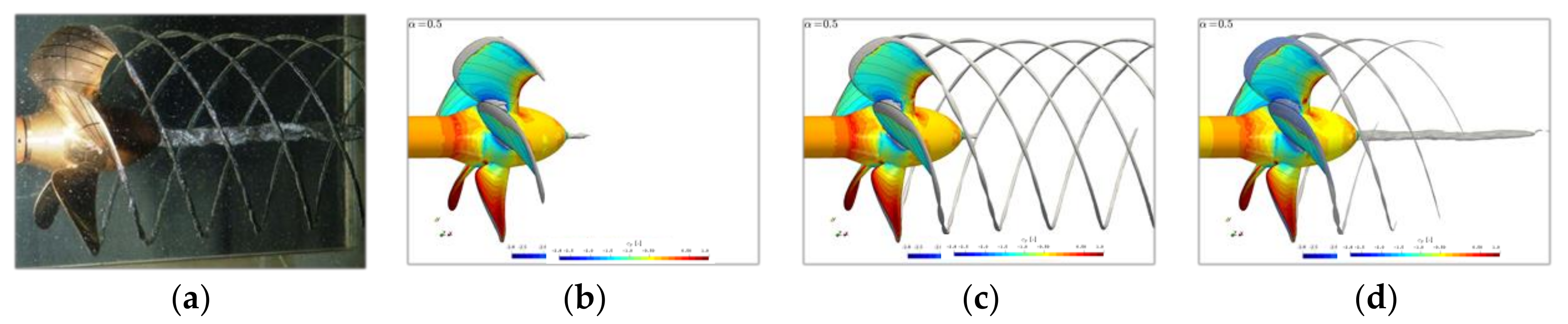
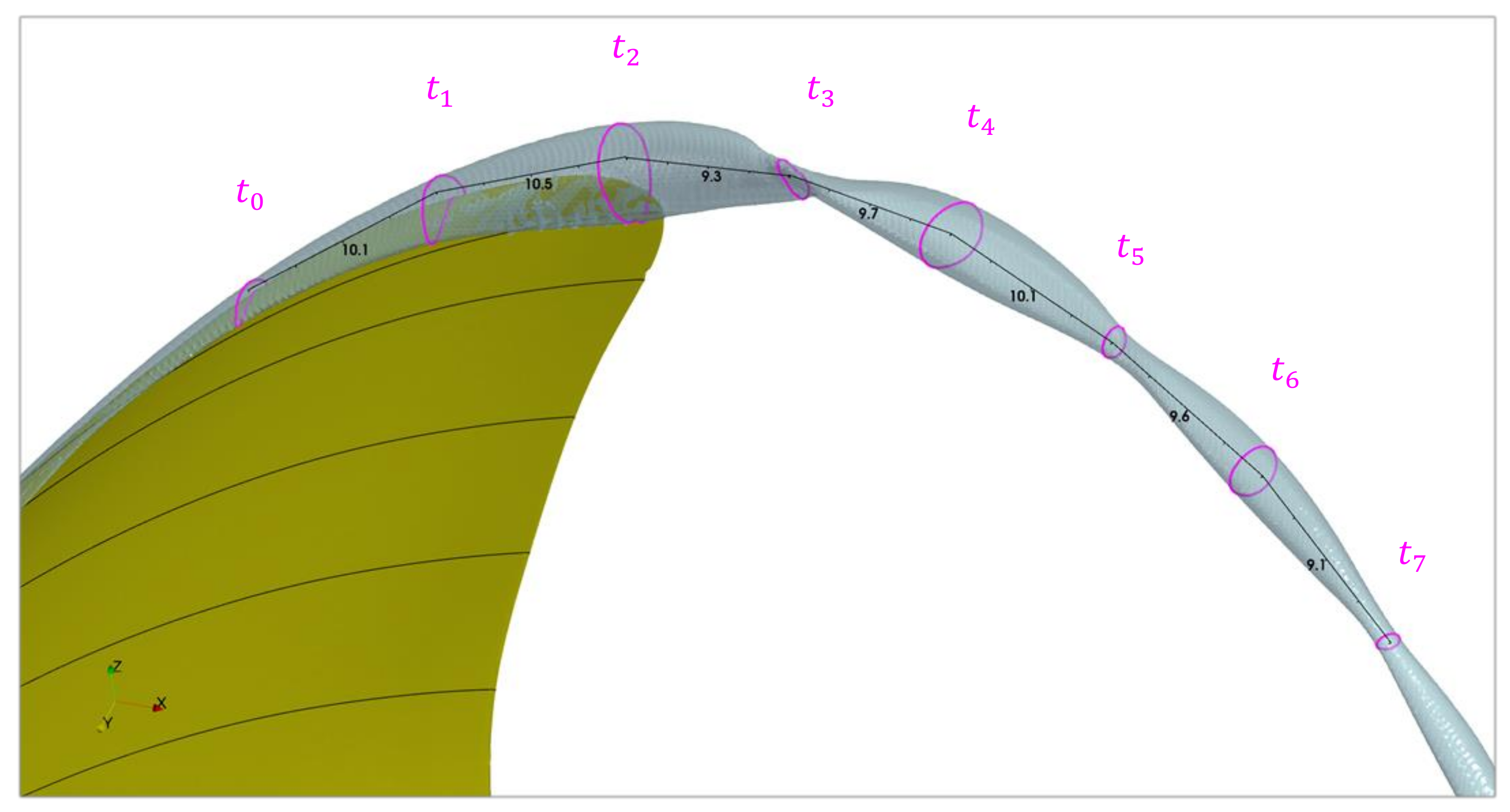
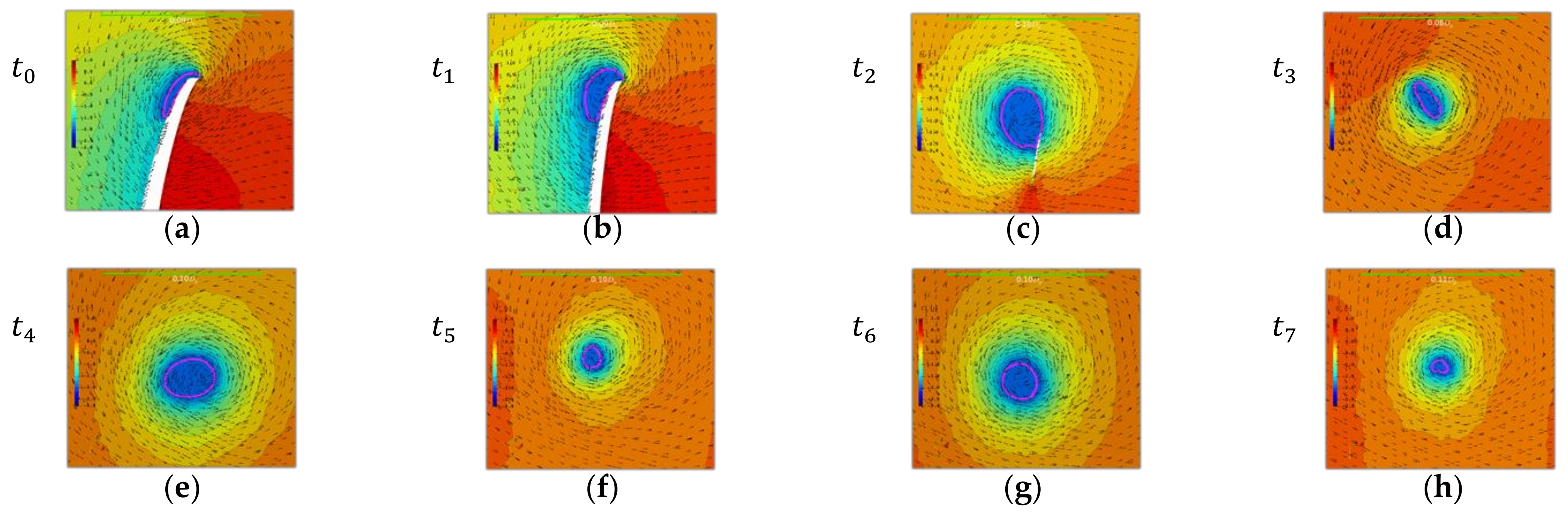
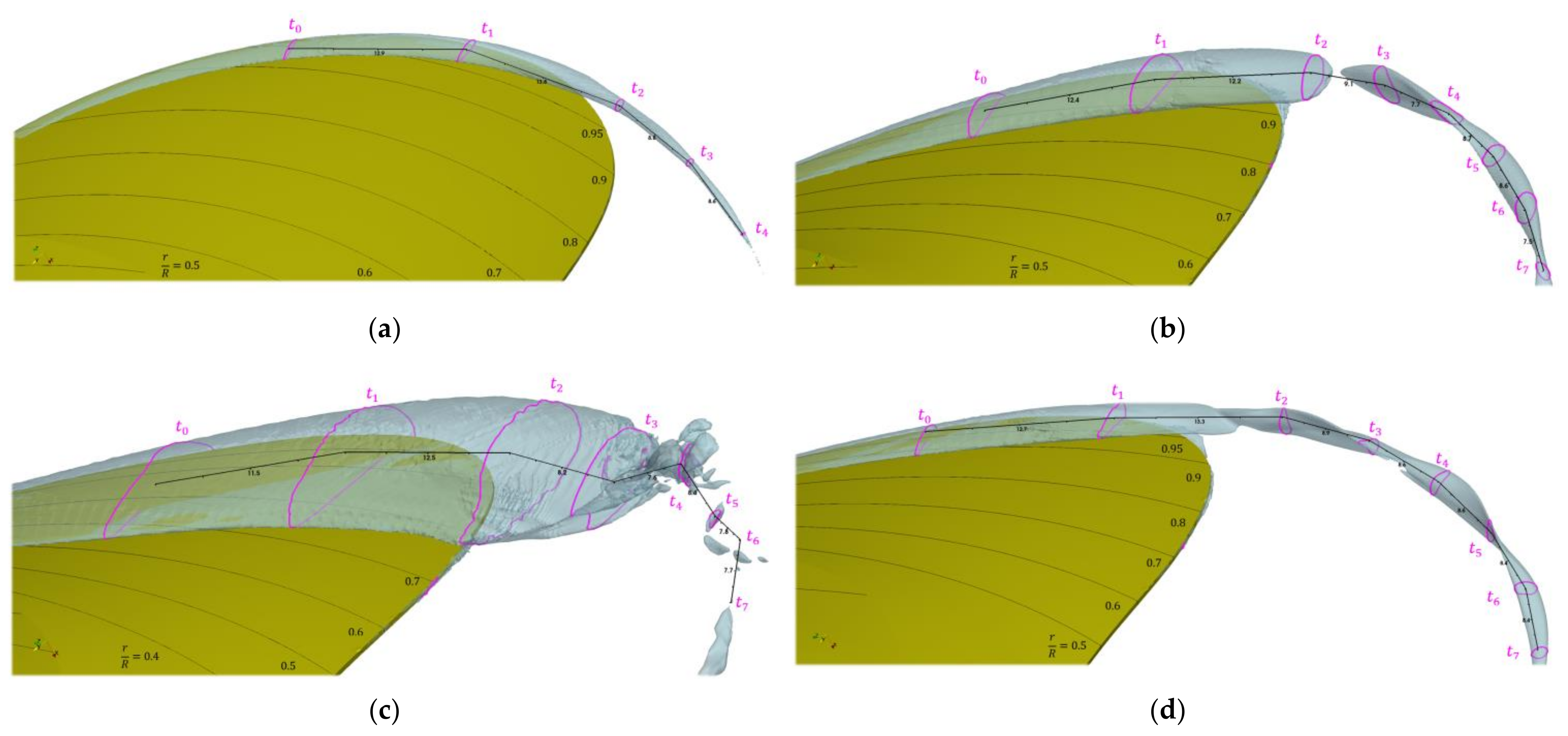
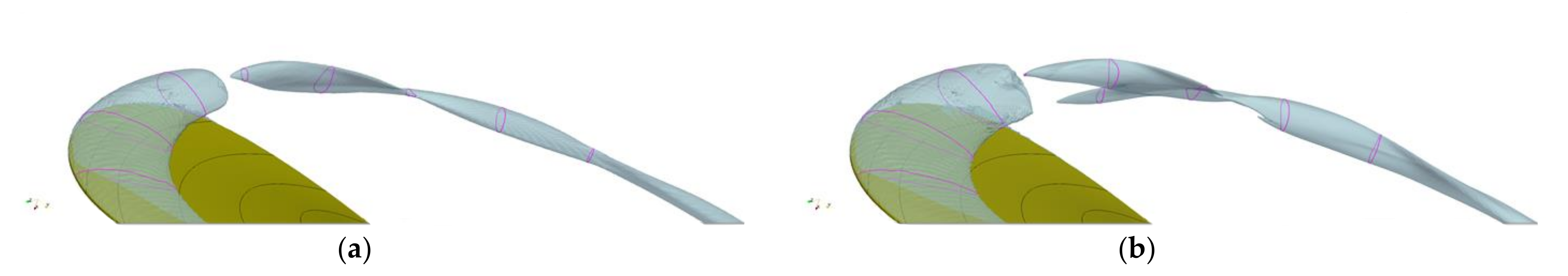
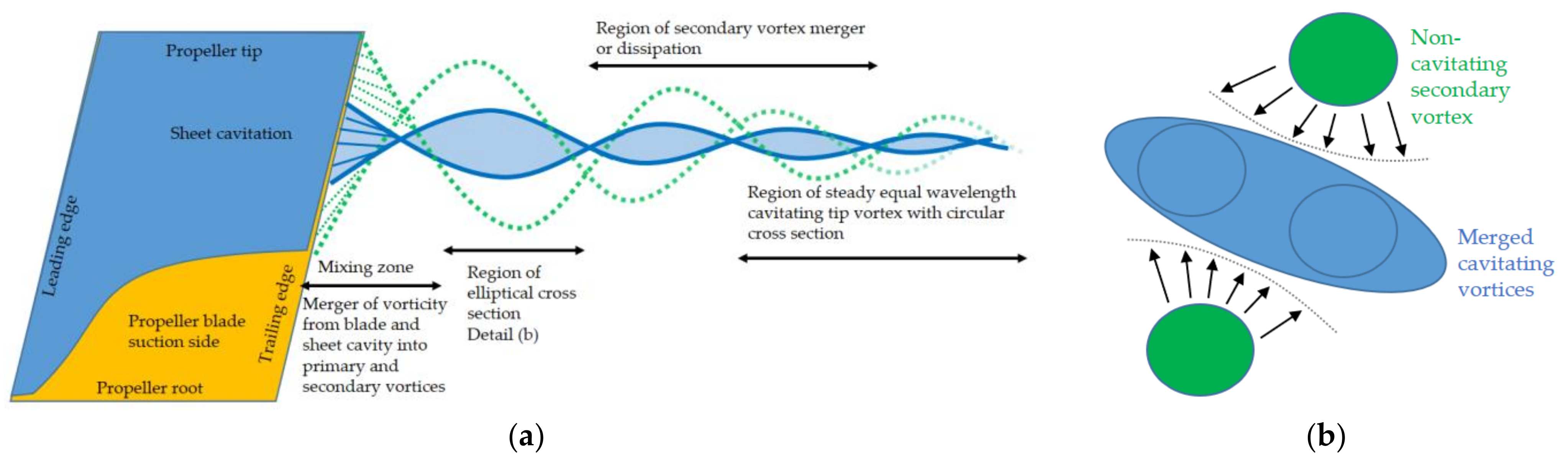
  • The source of the formation of the cavity is the reduced pressure due to the accelerated flow (a–c), in accordance with Bernoulli’s principle;
  • The assumed elliptical shape of the vortex is the result of the orientation of the detaching sheet along the blade surface;
  • The conserved angular momentum along the running length maintains the cavity diameter, in accordance with Kelvin’s circulation theorem;
  • The deformation of the ellipse to an energetically more favorable circular cross-sectional shape of the cavity takes place in the regions (d,e) vs. (f,g), as the surface tension is not considered in the Schnerr-Sauer model.
With the knowledge of the deforming cross-section of the vortex core along the running length, it is apparent that the introductory mentioned mesh requirements from the literature are difficult to comply with, even when the jet contraction is known a priori. Utilizing the resource-demanding a priory mesh refinement approach described, with the different core cross-section extent, especially in the elliptical stage of evolution, the criterion of Δ = 1 16 d , where d is the vortex core diameter [29], was not fulfilled for complex shapes of the enclosing streamline deviating from a simple circle, as the requirements are unfeasible for practical application. In Figure 7, the apparent violation of the criterion is visible for the semi-minor axis of the elliptical shape. These regions in the mixing zone of complex cavity formation, in particular, however, might have the most influential effect on its general shape and its initial evolution, as is shown in a simplified grid study in the Newcastle case. For the hub vortex in (c), the cell count was adequate, coming with the disadvantage of reduced stability.
Stations t 3 (a) and t 4 (b) are compared on the initial mesh without cavitation (noCav) to the final mesh result with cavitation activated (Cav AMR) in Figure 8, where two arbitrary lines through the assumed vortex core in the helix-normal planes are selected for U rel velocity plots. Nondimensionalisation of the position in the graphs obscures the non-axisymmetric vapor structure around the core, with its diameter as the axial distance between the maxima. Due to lack of material for validation, the velocity distribution was compared to a theoretical two-dimensional cylindrical Rankine vortex, depending only on its circulation Γ , which is determined with a relative velocity integral along a closed contour around the vortex core according to Stokes theorem,
Γ = C   u d l
.
The near-orthogonal lines intersect important flow features and the graph offsets have been shifted to coincide at the vortex center, determined by the minimum velocity. The contour and line plots reveal that the velocity magnitude was, contrary to the theory, quite asymmetric around the vortex core center. Nevertheless, the velocity distribution outside the vortex core followed a similar function as the analytical solution, described by the Rankine vortex. Similar to a noncavitating viscous core, the gaseous core seemed to follow the velocity distribution of a solid core rotation, as the velocity decreased linearly toward zero at the singular center for t 3 . For the downstream intersection t 4 , however, it appears that the vapor core had two velocity minima, which was distinctly seen for both lines in the graph and for L2 in the contour plot, which might be a residue of the initial elliptical vortex shape and orientation, being consumed by the gaseous phase. The initial noncavitating calculation featured no double minimum in the viscous core, which was presumably a result of the coarser mesh and not the inclusion of the gaseous phase.
The compactness c as a quotient of intersection area A and perimeter p , c = 4 π A / p 2 , of the α 0.5 isosurface with the helix normal planes is plotted over the nondimensionalized helix arc length based on the propeller diameter in Figure 9a to illustrate the cavity diameter and shape evolution along the tip vortex. Due to the surface interpolation based on a Delaunay algorithm, not all intersections were estimated correctly regarding the area, which led to some unphysical fluctuations, particularly when the cavity was still attached to the blade for values lower than the detachment point indicated by the dashed black line or the anti-nodes. At anti-nodes, the cavity cross-section appeared circular, whereas the cavity was elliptical at the nodes. The volume flow rate evolution inside the cavity, along the tip vortex, is in Figure 9b, where a positive value signifies a downstream direction flow perpendicular to the intersecting helix normal planes. In addition, the mass flow rate evolution based on the average mixture density ρ m = α l ρ l + 1 α l ρ g at the intersection is depicted and the above-mentioned stations t 0 to t 7 are marked in magenta. Within the cavity, the transfer of fluid was almost negligible at the nodes, while the transfer of mass was high at the anti-nodes, where the diameter of the cavity is large.
In Figure 10, the pressure midplane is evaluated for the final mesh, with the phase interface, together with pressure plots along equal-length vertical lines behind the propeller plane. While the pressure was almost constant across the core, just below the saturation pressure, it was independent of outside pressure, which seemed to approach a constant distribution shortly downstream of the initial hub vortex inception. For the lines intersecting tip vortex structures, a form of interaction between the hub and tip vortex in the pressure distribution was evident.

3.2. Newcastle Propeller Test Case

For the Newcastle propeller test case, the integral values for the considered simulations are listed in Table 7 with a slight improvement based on the switch of the pressure velocity coupling algorithm from PISO to PIMPLE compared to the PPTC’11 case, leading, in general, to a similar conclusion. For the J = 0.5 case, a steady-state frozen rotor setup based on a single phase-coupled solver with a kinematic pressure definition, which typically features high accuracy in combination with solution speed, was not able to reproduce the experimental values.
The initial meshes resulted in no tip vortex cavity for all cases, except an incipient structure for C2, similar to the PPTC’11 case. Employing the a priory refinement approach, tip vortex cavities, which were less defined than for the PPTC’11 case, formed in all cases, as illustrated in Figure 11. However, for C1, it did not extend very far beyond the blade surface, even though a cavitating tip vortex was prevalent in the experiment for more than one rotation behind the trailing edge. Therefore, a higher refinement level with eight times the cell count in the tip vortex region was applied, while a lower axial extent of the a priory vortex distance refinement for the remaining conditions was accepted. For C2, the sheet cavity transitioned into a tip vortex cavity with elongated cross-section, which was maintained over one spatial pulsation of the tip vortex core, developing further into a circular cross-section, which dissolved over the next half rotation, although it seemed to be stable in the experiment. C3 exhibited the largest sheet cavity on the blade, where in the observations, the sheet cavity seemed to turn into a detached unstable cloud cavity at the blade tip. While the cloud features could not be adequately modeled by the VOF-based formulation of phase interfaces in the simulation, the sheet cavity was detached from the blade starting near r R = 0.7 at the trailing edge side and being fully developed at the tip. Regardless, a remaining tip vortex filament was visible along the helix path for a short running length for the experiment, which was somewhat captured in the simulation, with multiple individual cavities of larger extent following the helical path of vorticity. The high advance ratio case C6, on the other hand, agreed very well with the cavitation test results, as both shape and extent were comparable. As cavities in C2 and C6 seemed to dissolve upon exiting the refined mesh region, it is unclear up to which extent the cavitating core can be maintained with the approach applied. It has to be noted that, during the simulation, a low-frequency pressure fluctuation was superimposed on the calculated pressure in the complete domain, possibly caused by pressure reflections at the domain boundaries, which, in turn, could be attributed to the small domain dimensions imposed by the experimental setup.
In Figure 12, all considered cases are investigated in an identical approach to the previous subsection, and the intersection with the helix-normal plane is highlighted. Note that the view is not identical for all images, as the best visibility for the intersection isolines has been considered. In all cases, a detached cavitation at the blade leading edge was visible, as well as an elliptically shaped initial cavity beyond the trailing edge at the start of the mixing zone. C1 (a) is the only case where the sheet cavity extended into the vortex cavity, which could be due to the coarser underlying mesh in this case. While C3 (c) experienced no clear structure, as several vapor blobs recombined after the mixing zone, C2 (b) and C6 (d) shared a topology for the tip vortex cavity, with a difference in the mixing zone, where C2 exhibited a completely disconnected sheet and tip vortex isosurface. C6 experienced a narrowing at the transition from sheet to tip vortex cavity. For C6, the isosurface began to collapse for the inner vertex of the elliptical shape, for instance, between station t 3 and t 4 in the figure. Clear nodes of periodicity for the vapor core pulsation along the helical running length were discernable for C2 and C6 with a wavelength of about λ = 0.15 D .
Introducing the vorticity isosurface representation in green in Figure 13, there are several noncavitating additional vortices visible, forming at the radial ends of the sheet cavity and circulating around the main cavitating vortex in a clockwise direction. While the exact underlying mechanisms of the vortex–vortex interaction were not clear from this simulation, these noncavitating secondary vortices circling around the cavity were connected to the elongated cross-section of the vapor cavity appearing for C2 and C6, where their trajectory left a related indentation. Further mesh refinement of case C2 compared in Figure 14 changed the topology of the primary vortex cavity into two separate cavitating tip vortices in the mixing zone and, in addition, increased the detached cavitation length of the suction side leading edge cavity on the blade, despite identical mesh settings in this region. Similar to the hub and tip vortex interaction based on the pressure distribution for the PPTC’11 case, an upstream pressure interaction between the tip vortex and the sheet cavity could be implied by this behavior. With this simulation setup, it could not be determined whether the structure in Figure 14b was a steady or unsteady condition or a periodic process, as the current limitation of resources rendered this approach unfeasible for long-term convergence observations and, additionally, the increased cell count came with a reduction in stability, leading to even higher calculation times. Comparing the results at downstream stations, it seems that the influence of the exact behavior in the mixing zone began to diminish with increasing running length.
The evolution of the shape and the flow rate normal to the cavity cross-section is shown in Figure 15 for cases C2 and C6, which developed a steady tip vortex cavitation. While the shape evolution was slightly different, the general findings remained the same. Beyond the blade in the mixing zone, the cavity assumed a very elliptical form and, in the case of C2 (a), even reached zero as a result of the nonexistent cavity along a few data points. The evaluation of the flow rates confirmed that there was no significant transfer along the cavity axis, only within anti-nodes with large diameters, which can be interpreted as pockets of high mass-transfer moving along the helix and not interacting with the neighboring cavities.

4. Discussion

4.1. Forces Prediction

The investigated simulation method with ILES, without a wall model and with an a priory mesh refinement in combination with the Schnerr–Sauer cavitation model, should in practice be quicker than other LES and DES methods with comparable levels of cavity details, due to a lower cell count and reduced number of equations, as well as not requiring a RANS-LES interface interpolation. As expected, investigations for one operation condition of the PPTC’11 and four for the Newcastle propeller test case produced only a moderate accuracy regarding the prediction of integral thrust. In particular, the propeller flow simulations under consideration of the cavitation showed differences in thrust with values > 5 % , which is too high for practical use. Primarily, the reason may be the missing wall model in the ILES. In addition to the large y + values that take place in the Newcastle case, a second reason for the difference in propeller thrust may be the small number of external correction iterations used. A more physical reason that could explain the larger difference of the results for the cavitating flow part of the study could be the different sheet cavity structures compared to the experiment. In the cases studied, the differences were high and it is, thus, not recommended to conclude the integral values from these calculations, which, however, is not necessary, as the required preceding RANS calculation produced good results. The source of the large differences needs to be studied in detail, as the ILES approach is able to produce accurate results [17].

4.2. Noise Generation Mechanisms

The overall cavitation pattern structures were, from a purely visual comparison, in good agreement with the experiments, when appropriate mesh refinements were implemented in regions of high vorticity. The proposed natural modes of vibration shown in Figure 1 for the cavitating tip vortex phase interfaces originating from suction side sheet cavitation at the propeller leading edge could not be observed in the simulations with temporal analyses with videos of the α 0.5 isosurfaces with a sampling frequency of f s = 9 kHz. Detecting any vibrations might require larger sampling frequencies in the model scale or the Schnerr–Sauer cavitation model, and could be insufficient as a result of the missing higher-order terms of the linearized Rayleigh–Plesset Equation. However, depending on the helical structure, described by the tip vortex, steady shapes could be identified along a limited running length that resemble these modes. Physical mechanisms such as a spatially pulsating vapor vortex core along the running length and conservation of angular momentum around the core could be reproduced. According to the results of the Newcastle simulation, noncavitating secondary tip vortices, originating at the radial outer ends of the sheet cavity and spinning in a circular motion, around the center cavity along its streamwise running length, were responsible for compressing the primary cavity flow cross-section into an elliptical shape. Furthermore, it seems that the primary cavitating core was composed of at least two internal vortices, contributing to the formation of the elliptical cavity shape. In fact, higher mesh resolutions were required to investigate whether these vortices were raised from a separate origin in the mixing zone. It was proposed that a tip vortex, as any cavitating vortex, assumes the energetically superior mode n = 0 , when additional vortices are no longer constraining the shape, by physical or numerical dissipation or merging with the primary vortex structure. In Figure 16, dual vortex cores of the cavity (blue), which could be a result of several smaller vortices generated at the end of the sheet cavities end and merged in the mixing zone, and their consecutive interaction with the secondary vortices (green) are schematized.
As long as no corresponding validation material with detailed geometry descriptions of the tip vortex phase interface is available, the presented hypothesis, based solely on CFD simulations, needs additional evidence, which can only be achieved by future intensive research efforts. On the numerical side, improved meshing strategies are necessary, as the resource demand regarding mesh refinement in the investigated propeller slipstream regions are currently the only limiting factor for further exploration of the topic with the proposed approach. While the results display a high level of detail, a mesh independence study is essential.

5. Conclusions

The proposed approach for determining the acoustic sources of a propeller in the behind-ship condition with ILES without the wall model in combination with the VOF-method and the Schnerr–Sauer cavitation model is suggested as a computationally less expensive alternative to traditional LES or DES methods. For this approach, as expected, the prediction of integral values of the propeller was inferior to the former or the RANS method, especially regarding the prediction of forces. A further improvement of the cavitation modeling in the tip and hub vortex region, which are expected to influence acoustic emissions, is suggested with a single Q-criterion-based refinement step, corresponding to a sufficiently high vorticity value, in order to keep the number of cells low and only refine the cavitating tip vortex. After the a priory refinement, the maximum details of noise generation mechanisms in a free running propeller slipstream were resolved, with the remaining restrictions enforced by the VOF-method and the Schnerr–Sauer cavitation model. By comparing different hub vortex refinement levels, a strong interaction between the tip and hub vortex cavities was determined. The proposed approach was only partly viable, when the flow at the propeller was not straight and a solid structure interacted with the propeller slipstream, which is typically the case in the behind-ship condition for traditional propellers.
Summarizing, the proposed approach fulfils the initial expectations and could be a feasible way to estimate URN with high-fidelity CFD methods in an industry environment. However, the acoustic pressure prediction in the near field and its comparison with the hydrodynamic pressure of the FVM must be compared in order to validate the approach’s feasibility for the intended purpose.

Author Contributions

Conceptualization, M.A.-M.; methodology, J.K.; investigation, J.K.; resources, P.M.; data curation, J.K.; writing—original draft preparation, J.K.; writing—review and editing, M.A.-M. and P.M.; visualization, J.K.; supervision, M.A.-M.; project administration, P.M.; funding acquisition, P.M. All authors have read and agreed to the published version of the manuscript.

Funding

This research was funded by the European Union’s Horizon 2020 research and innovation programme under grant agreement No. 728053-MarTERA, represented by BMWi in Germany, grant number 03SX461C as part of the ProNoVi joint research project.

Institutional Review Board Statement

Not applicable.

Informed Consent Statement

Not applicable.

Acknowledgments

The partners in the ProNoVi project, namely SINTEF Ocean, CNR-INM, Fr. Lürssen Werft GmbH and Co. KG, and Helseth AS, are acknowledged for the support of this work with their contributions to the discussion and the scientific exchange.

Conflicts of Interest

The authors declare no conflict of interest. The funders had no role in the design of the study; in the collection, analyses, or interpretation of data; in the writing of the manuscript, or in the decision to publish the results.

References

  1. Van Wijngaarden, H.C.J. Prediction of Propeller-Induced Hull-Pressure Fluctuations; Maritime Research Institute Netherlands: Wageningen, The Netherlands, 2011. [Google Scholar]
  2. Berger, S. Numerical Analysis of Propeller-Induced Higher-Order Pressure Fluctuations on the Ship Hull; Schriftenreihe Schiffbau der Technischen Universität Hamburg-Harburg: Hamburg, Germany, 2018. [Google Scholar]
  3. Bosschers, J. Analysis of inertial waves on inviscid cavitating vortices in relation to lowfrequency radiated noise. In Proceedings of the Warwick Innovative Manufacturing Research Centre (WIMRC) Cavitation: Turbo-machinery and Medical Applications Forum, Coventry, UK, 7–9 July 2008. [Google Scholar]
  4. Asnaghi, A.; Bensow, R.E.; Svennberg, U. Comparative analysis of tip vortex flow using RANS and LES. In Proceedings of the VII International Conference on Computational Methods in Marine Engineering, Nantes, France, 15–17 May 2017. [Google Scholar]
  5. Bensow, R.E.; Liefvendahl, M. An acoustic analogy and scale-resolving flow simulation methodology for the prediction of propeller radiated noise. In Proceedings of the 31st Symposium on Naval Hydrodynamics, Monterey, CA, USA, 11–16 September 2016. [Google Scholar]
  6. Bensow, R.; Liefvendahl, M. Implicit and Explicit Subgrid Modeling in LES Applied to a Marine Propeller. Proceeding of the 38th fluid dynamics conference and exhibit, Siattle, DC, USA, 23–26 June 2008. [Google Scholar]
  7. Kimmerl, J.; Mertes, P.; Krasilnikov, V.; Koushan, K.; Savio, L.; Felli, M.; Abdel-Maksoud, M.; Göttsche, U.; Reichstein, N. Analysis Methods and Design Measures for the Reduction of Noise and Vibration Induced by Marine Propellers; Universitätsbibliothek der RWTH Aachen: Aachen, Germany, 2019. [Google Scholar]
  8. Asnaghi, R.E. Implicit Large Eddy Simulation of Tip Vortex on an Elliptical Foil. In Proceedings of the Fifth International Symposium on Marine Propulsion, Espoo, Finland, 12–15 June 2017. [Google Scholar]
  9. Tani, G.; Aktas, B.; Viviani, M.; Atlar, M. Two medium size cavitation tunnel hydro-acoustic benchmark experiment comparisons as part of a round robin test campaign. Ocean Eng. 2017, 138, 179–207. [Google Scholar] [CrossRef] [Green Version]
  10. Krasilnikov, V. CFD modelling of hydroacoustic performance of marine propellers: Predicting propeller cavitation. In Proceedings of the 22nd Numerical Towing Tank Symposium, Tomar, Portugal, 29 September–1 October 2019. [Google Scholar]
  11. Kuiper, G. Cavitation Inception on Ship Propeller Models. Ph.D. Thesis, TU Delft, Wageningen, The Netherlands, 1981. [Google Scholar]
  12. Viitanen, V.M.; Hynninen, A.; Sipilä, T.; Siikonen, T. DDES of Wetted and Cavitating Marine Propeller for CHA Underwater Noise Assessment. J. Mar. Sci. Eng. 2018, 6, 56. [Google Scholar] [CrossRef] [Green Version]
  13. Sagaut, P. Large Eddy Simulation for Incompressible Flows; Springer: New York, NY, USA, 2006. [Google Scholar]
  14. Arndt, R.E.A.; Arakeri, V.H.; Higuchi, H. Some observations of tip-vortex cavitation. J. Fluid Mech. 1991, 229, 169–289. [Google Scholar] [CrossRef]
  15. Felli, M.; Falchi, M. Propeller tip and hub vortex dynamics in the interaction with a rudder. Exp. Fluids 2011, 51, 1385–1402. [Google Scholar] [CrossRef] [Green Version]
  16. Zhang, G.; Khlifa, I.; Fezzaa, K.; Ge, M.; Coutier-Delgosha, O. Experimental investigation of internal two-phase flow structures and dynamics of quasi-stable sheet cavitation by fast synchrotron X-ray imaging. Phys. Fluids 2020, 32, 113310. [Google Scholar] [CrossRef]
  17. Van Terwisga, T.J.; Li, Z.R.; Fitzsimmons, P.A.; Foeth, E.J. Cavitation Erosion—A review of physical mechanisms and erosion risk models. In Proceedings of the 7th International Symposium on Cavitation, Ann Arbor, MI, USA, 16–20 August 2009. [Google Scholar]
  18. Sezen, S.; Atlar, M.; Fitzsimmons, P. Prediction of cavitating propeller underwater radiated noise using RANS & DES-based hybrid method. Ships Offshore Struct. 2021. [Google Scholar] [CrossRef]
  19. Yilmaz, N.; Atlar, M.; Fitzsimmons, P. An Improved Tip Vortex Cavitation Model for Propeller-Rudder Interaction. In Proceedings of the 10th International Cavitation Symposium, Baltimore, MD, USA, 13–16 May 2018. [Google Scholar]
  20. Viitanen, V.; Siikonen, T.; Sánchez-Caja, A. Cavitation on Model- and Full-Scale Marine Propellers: Steady and Transient Viscous Flow Simulations at Different Reynolds Numbers. J. Mar. Sci. Eng. 2020, 8, 141. [Google Scholar] [CrossRef] [Green Version]
  21. Bretschneider, H.; Bosschers, J.; Choi, G.H.; Ciappi, E.; Farabee, T.; Kawakita, C.; Tang, D. Specialist Committee on Hydrodynamic Noise. In Proceedings of the Final report and recommendations to the 27th ITTC, Copenhagen, Denmark, 31 August–5 September 2014. [Google Scholar]
  22. International Maritime Organization. Guidelines for the Reduction of Underwater Noise from Commercial Shipping to Address Adverse Impacts on Marine Life; International Maritime Organization: London, UK, 2014. [Google Scholar]
  23. DNV GL. Silent Class Notation; DNV GL AS: Bærum, Norwegen, 2010. [Google Scholar]
  24. Viitanen, V.; Siikonen, T.; Sánchez-Caja, A. Numerical Viscous Flow Simulations of Cavitating Propeller Flows at Different Reynolds Numbers. In Proceedings of the Sixth International Symposium on Marine Propulsors, Rome, Italy, 26–30 May 2019. [Google Scholar]
  25. Kimmerl, J.; Mertes, P.; Abdel-Maksoud, M. Turbulence Modelling Capabilities of ILES for Propeller Induced URN Prediction. In SNAME Maritime Convention; SNAME: Houston, TX, USA, 2020. [Google Scholar]
  26. Menter, F.R. Best Practice: Scale-Resolving Simulations in ANSYS CFD; ANSYS Germany GmbH: Nürnberg, Germany, 2015. [Google Scholar]
  27. Krasilnikov, V.; Abdel-Maksoud, M.; Göttsche, U.; Wang, Y.; Koushan, K.; Kimmerl, J.; Mertes, P.; Felli, M.; Reichstein, N.; Stück, R.; et al. Study on Analysis Methods for Marine Propeller Cavitation and the Radiated Noise; Hauptversammlung der Schiffbautechnischen Gesellschaft: Papenburg, Germany, 2019. [Google Scholar]
  28. SVA Potsdam GmbH. Potsdam Propeller Test Case (PPTC)—Cavitation Tests with the Model Propeller VP1304; Report 3753, Online; Schiffbau-Versuchsanstalt: Potsdam, Germany, 2011. [Google Scholar]
  29. Tani, G.; Viviani, M.; Felli, M.; Lafeber, F.H.; Lloyd, T.; Aktas, B.; Atlar, M.; Seol, H.; Hallander, J.; Sakamoto, N.; et al. Round Robin Test on Radiated Noise of a Cavitating Propeller. In Proceedings of the Sixth International Symposium on Marine Propulsors, Rome, Italy, 20 May 2019. [Google Scholar]
Figure 1. Different modes of a vibrating core vortex: (a) breathing mode n = 0 ; (b) bending mode n = 1 ; (c) double helix mode n = 2 , where n is the azimuthal wave number based on the formulation in a cylindrical coordinate system, reproduced from [9] with permission from Verlag Schriftenreihe Schiffbau, year 2021.
Jmse 09 00792 g001
Figure 2. Initial mesh: (a) PPTC’11; (b) Newcastle.
Jmse 09 00792 g002
Figure 3. PPTC’11. Distance refinement in tip vortex region: (a) first mesh refinement step based on Q -criterion Q = 5 10 4 s 2 ; (b) second mesh refinement step based on α = 0.5 with additional hub vortex refinement.
Jmse 09 00792 g003
Figure 4. PPTC’11. (a) Experiment, reproduced from [26], with permission from SVA Potsdam, 2021; (b) initial mesh; (c) mesh refinement 1; (d) mesh refinement 2.
Jmse 09 00792 g004
Figure 5. PPTC’11. Tip vortex cavitation isosurface with investigated stations and normalized arc length approximation along helix.
Jmse 09 00792 g005
Figure 6. PPTC’11. (ah) Relative velocity plots with pressure contours in helix-normal plane at stations t 0 t 7 , respectively, with phase interface in magenta.
Jmse 09 00792 g006
Figure 7. PPTC’11. Mesh comparison: (a) helix-normal plane station t 3 ; (b) helix-normal plane station t 4 ; (c) shaft-normal plane at x = 0.4 D P .
Jmse 09 00792 g007
Figure 8. PPTC’11. Comparison of relative in-plane velocity with inviscid 2D analytical vortices angular velocity: (a) station t 3 ; (b) station t 4 .
Jmse 09 00792 g008
Figure 9. PPTC’11. Tip vortex longitudinal evolution analysis: (a) shape; (b) flow rate.
Jmse 09 00792 g009
Figure 10. PPTC’11. Pressure distribution in the slipstream: (a) pressure contours in midplane with investigated lines; (b) pressure plots along investigated lines.
Jmse 09 00792 g010
Figure 11. Newcastle. Comparison with experiment, reproduced from [15], with permission from Elsevier, year 2021: (a) C1; (b) C2; (c) C3; (d) C6.
Jmse 09 00792 g011
Figure 12. Newcastle. Tip vortex cavitation isosurface with stations and normalized arc length approximation along helix: (a) C1; (b) C2; (c) C3; (d) C6.
Jmse 09 00792 g012
Figure 13. Newcastle. Tip vortex isosurfaces for cavitation α 0.5 (blue) and Q-criterion Q = 5 10 4   s 2 (green): (a) overview; (b) single vortex view.
Jmse 09 00792 g013
Figure 14. Newcastle. C2 tip vortex cavitation isosurface with two stations and two different refinement levels: (a) Base a priory; (b) 8× higher cell count in the tip vortex region.
Jmse 09 00792 g014
Figure 15. Newcastle. Tip vortex longitudinal evolution analysis: (a) C2: shape; (b) C2: flow rate; (c) C6: shape; (d) C6: flow rate.
Jmse 09 00792 g015
Figure 16. Possible mechanisms of tip vortex cavity shape formation: (a) unwrapped lateral view; (b) cross-section detail.
Jmse 09 00792 g016
Table 1. Parameters of the Schnerr–Sauer cavitation model.
Parameter n 0 d Nuc
Unit 1 / m 3 m
Value 1 10 12 1 10 4
Table 2. Newcastle test case. Considered test conditions from round-robin test.
ConditionC1C2C3C6
J   0.4 0.4 0.4 0.5
σ n   2.22 1.3 0.72 1.13
n [Hz]35353535
Table 3. PPTC’11. Effect of time step size on the propeller slipstream vorticity for an identical mesh without mesh refinement step at J = 1.019 , partly based on [25].
TypeStep
[°]
Q-Isovalue of Q = 5 10 4 s 2 with Axial Velocity CFL
[-]
Effort (2 rot/100 CPUs)
[d]
RANS10 Jmse 09 00792 i0011.38–550.490.1
RANS1 Jmse 09 00792 i0020.13–72.380.32
RANS0.1 Jmse 09 00792 i0030.01–7.333.4
ILES1 Jmse 09 00792 i0040.13–66.200.4
ILES0.1 Jmse 09 00792 i0050.01–6.953.0
ILES0.1 Jmse 09 00792 i0060.001–0.6628.0
Table 4. Newcastle. Effect of different time steps on the propeller slipstream vorticity with ILES for Newcastle propeller.
Step
[°]
Q-Isovalue of Q = 5 10 4 s 2 with Axial Velocity CFE
[-]
Effort (2 rot/100 CPUs)
[d]
0.33 Jmse 09 00792 i0070.03–11.510.72
0.1 Jmse 09 00792 i0080.00–3.441.87
Table 5. Overview of the meshes for each case with applied refinement steps.
Cell Count [ 10 6 Cells]
MeshPPTC’11Newcastle
Initial mesh 11.4 13.0
Refinement step 1 65.2 C1: 32.3
C2: 24.9
C3: 27.5
C6: 40.1
Refinement step 2 35.5 -
Table 6. PPTC’11. Integral values at J = 1.019 .
Investigation k T [-] Δ [%] 10 k Q Δ [%]
Experiment (Cav Off)0.381-0.976-
Experiment (Cav On)0.374-0.970-
RANS k-ω-SSTawt: tdiCoupled (Cav Off)0.3810.11.0083.3
ILES: pimpleDyMFoam (Cav Off)0.3964.10.9951.9
LES Sm..: interPhaseChangeDyMFoam (Cav Off)0.3830.41.0275.2
ILES: interPhaseChangeDyMFoam (Cav On)0.42914.90.9952.6
Table 7. Integral values at J = 0.4 and J = 0.5 , Newcastle propeller test case.
Investigation k T [-] Δ [%] 10 k Q Δ [%]
J = 0.4 -Condition: C1, C2, C3
Experiment0.242-0.341-
RANS k-ω-SST: sdiCoupled
(steady, Cav Off)
0.243−0.60.3400.3
ILES: interPhaseChangeDyMFoam
(Cav On)
0.2314.60.3580.9
J = 0.5 -Condition: C6
Experiment0.190-0.284-
RANS k-kl-ω: interPhaseChangeDyMFoam (Cav Off)0.182−4.10.271−4.5
ILES: interPhaseChangeDyMFoam
(Cav On)
0.2047.20.31811.9
Publisher’s Note: MDPI stays neutral with regard to jurisdictional claims in published maps and institutional affiliations.

