Round Robin Laboratory Testing of a Scaled 10 MW Floating Horizontal Axis Wind Turbine

Abstract

This paper documents the round robin testing campaign carried out on a floating wind turbine as part of the EU H2020 MaRINET2 project. A 1/60th scale model of a 10 MW floating platform was tested in wave basins in four different locations around Europe. The tests carried out in each facility included decay tests, tests in regular and irregular waves with and without wind thrust, and tests to characterise the mooring system as well as the model itself. For the tests in wind, only the thrust of the turbine was considered and it was fixed to pre-selected levels. Hence, this work focuses on the hydrodynamic responses of a semi-submersible floating foundation. It was found that the global surge stiffness was comparable across facilities, except in one case where different azimuth angles were used for the mooring lines. Heave and pitch had the same stiffness coefficient and periods for all basins. Response Amplitude Operators (RAOs) were used to compare the responses in waves from all facilities. The shape of the motion RAOs were globally similar for all basins except around some particular frequencies. As the results were non-linear around the resonance and cancellation frequencies, the differences between facilities were magnified at these frequencies. Surge motions were significantly impacted by reflections leading to large differences in these RAOs between all basins.

1. Introduction

The offshore wind industry has seen remarkable advances over the last decade. Europe now has over 25 GW of installed offshore wind capacity, of which 2.9 GW was installed in 2020. Bottom-fixed turbines account for the majority of offshore wind capacity; floating wind accounts for only 62 MW at present1. As the industry develops and energy demands increase, turbines are getting larger and moving further from shore to take advantage of higher wind speeds. This trend presents significant technical challenges due to the deeper waters and the increasingly dynamic wind and wave conditions encountered. Therefore a key research area is the development of floating platforms and mooring systems that can withstand the enormous forces generated by increasingly large turbines in rough seas. The early stages of this development process involves testing models at a reduced scale in a laboratory setting, e.g., a wave basin. For a floating wind platform, wave basin testing typically involves still water decay tests, tests in regular and irregular waves with and without wind emulation, tests to characterise the mooring system and tests on dry land to characterise the model itself (e.g., the moments of inertia (MoI) and the centre of gravity (CoG)). During tank testing, motions of the model in each of the six degrees of freedom (DOF), i.e., surge, sway, heave, roll, yaw and pitch, are measured to determine how the platform responds to a range of wind and wave conditions. Thus wave basin testing allows for the validation of numerical models as well as characterising the full-scale dynamics of proposed prototypes. Furthermore, model testing is often the first opportunity to carry out a simplified, but global, assessment of the whole system (i.e., modelling the moored floater and the turbine together) [1].

Scaled model testing is an integral part of the development process for many offshore renewable energy (ORE) technologies, not just offshore wind. Testing at small scale can be efficient and relatively inexpensive, while testing within a controlled environment enables experiments to be repeated for a range of parameters. An additional advantage of testing at small scales is that each individual subsystem can be independently tested. However, the effects that a facility or laboratory will have on the outcomes even when following the same methodologies are uncertain.

The EU H2020 MaRINET2 project2 aims to improve the quality, robustness and accuracy of physical modelling and testing practices implemented by test infrastructures. Research carried out within MaRINET2 [2,3] identified a shortfall in the published guidance available for laboratory testing of floating offshore wind turbines (FOWTs). Much of the existing literature is derived from the oil and gas industry and published by the ITTC in the 7.5-02-07-03 series that deals with ocean engineering3. The ITTC guidelines are relatively high level and do not provide standardised procedures for laboratory testing or detailed guidance on different aspects of FOWT testing. Other sources of guidance for FOWT laboratory testing are published research articles that document individual tank testing campaigns but these are device and basin specific and may not provide relevant advice for an individual embarking on a tank testing campaign. Researchers involved in laboratory testing of FOWTs are often prevented from publishing detailed accounts and lessons learned from a test campaign by Intellectual Property (IP) restrictions. There is no published research on how the facility itself may impact the outputs of a laboratory testing campaign, and how to conduct tests in a way that the tester can have confidence that the results can be reproduced with good accuracy in another wave basin.

MaRINET2 is addressing these issues through a round robin testing program whereby generic wave, floating wind, and tidal devices are tested in different infrastructures. The purpose of the round robin tests is to assess the impact the facility itself has on the experimental results and provide recommendations on laboratory testing methodologies with a view to ultimately developing standardised testing processes for ORE devices. Another key output is the delivery of the datasets produced during each round robin test (see details at the end of the paper). MaRINET2 builds on the EU FP7 MARINET project which concluded in 2015. A tidal round robin campaign was conducted in MARINET [4] and a wave round robin was attempted, albeit unsuccessfully. In MaRINET2, the tidal round robin has been further developed [5,6], a successful wave round robin featuring two devices has been conducted [7,8] and a first attempt is made at round robin testing of a floating wind platform.

This paper documents the floating wind campaign which was conducted at four facilities: Ifremer and Centrale Nantes (ECN) in France, the University of Strathclyde (UoS) in the UK and University College Cork (UCC), Ireland. This experimental study is a true round robin test of a FOWT where different basins, teams and procedures are used to test the same test specimen. At least one comparison of tests of a FOWT model in different basins has already been carried out and documented in [9]. However, the latter tests were carried out by a single laboratory (thus following the same testing procedures). Morever, the model was not strictly identical in [9] but each test series included some variations in the mass distribution and the mooring system. In the present FOWT round robin testing campaign, the same test plan was shared between all facilities and a large number of tests were completed in all basins. This enables a fair comparison of model-test results with a sharper focus on the effects of the basin and the testing methods employed. The emphasis in this paper is more on the analysis of the results and less on the reporting of the method employed by each facility.

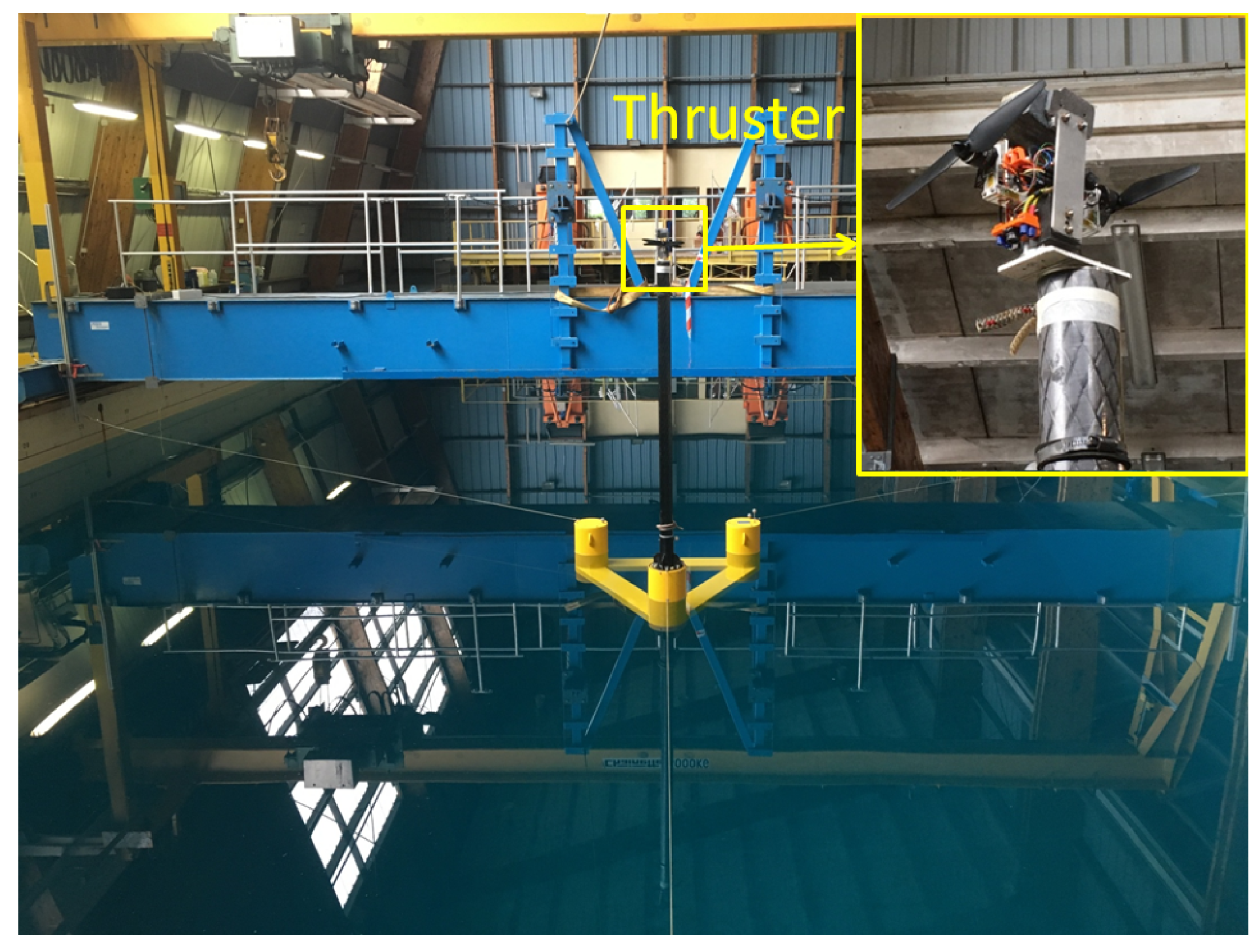
2. Model and Instrumentation Details

The test specimen is based on a 10 MW semi-submersible floating horizontal axis turbine, designed originally by CENER as part of the INNWIND.EU project [10]. The structure comprises 3 cylindrical columns connected by horizontal rectangular pontoons. The turbine tower is mounted on the aft column and is designed to host a variety of turbine simulators. The 1/60th scale model has an aluminium hull with a carbon fibre composite tower as shown in Figure 1, with dimensions shown in Figure 2. The platform is aerially moored in a horizontal alignment with spring enable mooring lines connected from each tower to the tank walls of the wave basins. This model has travelled in all facilities for the round robin testing.

The round robin testing programme explores various methods of wind emulation including a scaled rotor, a uni-directional thruster and a simple weighted pulley system. This research paper presents the results obtained from using the thruster only which is shown in Figure 1. The thruster was provided by Ifremer, and calibrated and programmed to achieve fixed values of thrust (3, 5, 7 and 8 N). The force delivered by this thruster is perpendicular to the virtual wind turbine rotor plane and applied at the wind turbine hub’s location. In a real wind turbine, forces and moments in three directions would act at this point rather than only one (i.e., the thrust). However, the thrust is the most important wind load component for the design of a floating foundation for several reasons:

• It causes a horizontal drift motion that affects the tension in the mooring lines.
• Due to the height at which the thrust is exerted, the moment around the CoG of the platform is very large and often causes the platform to rotate. Under the steady thrust levels that are the investigated in the present study, the submerged geometry of the floater will vary and this could influence its response to waves.
• When the thrust varies under the combined effects of the wind, the platform’s motions and the wind turbine controller, these variations have a direct effect on the motions of the floater by modifying the level of damping. This effect is not accounted for in the present test set-up as the thrust is constant when active.

Despite the simplification brought by this thruster, it still enables exploration of the essential aspects of the impact of the wind turbine loads on the hydrodynamic response of the floater.

3. Facility Details and Experimental Setup

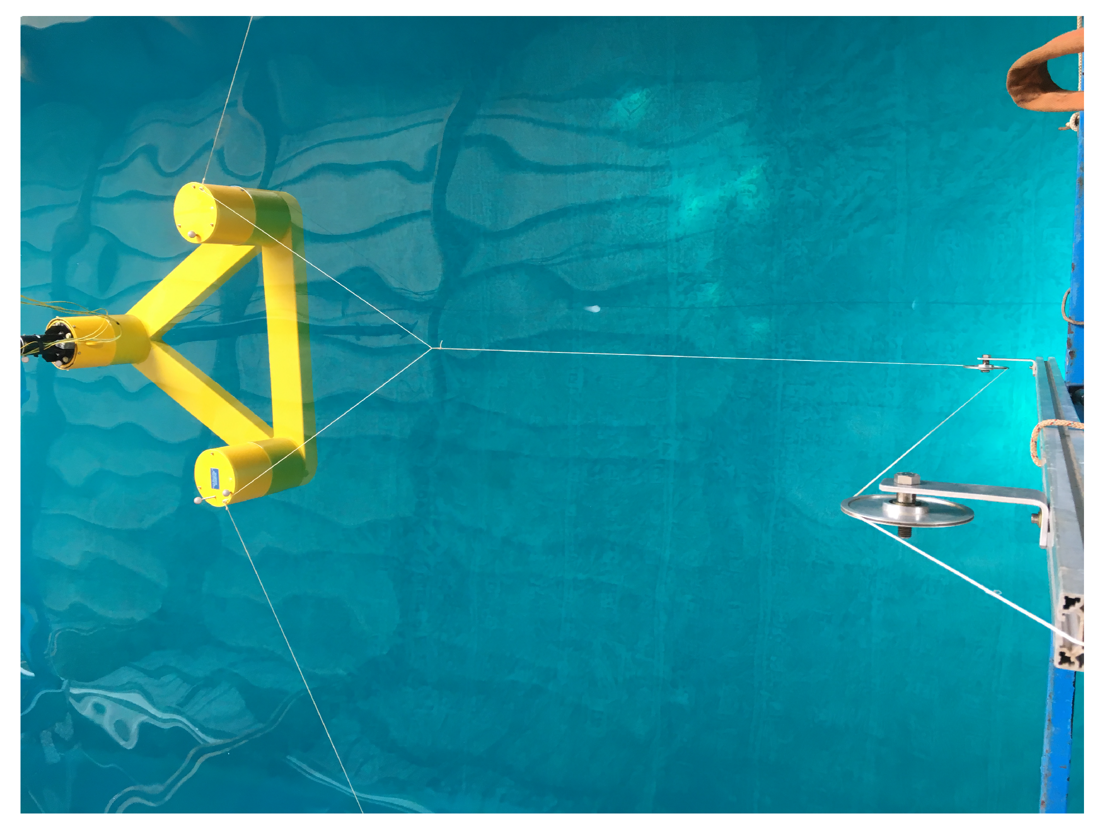
Five tests at four facilities were carried out as part of the round robin test program: Ifremer, Centrale Nantes (ECN), University of Strathclyde (UoS) and two tests at University College Cork (UCC). The primary purpose of the second test at UCC was to test a second method of wind emulation a number of months after the original test. However, the original test plan with (and without) the thruster was also partly repeated. These latter results comprise the fifth dataset used in the present research paper. The main features of the wave basins in each facility are given in

Table 1. Features of the test facilities. ‘Label’ indicates how the datasets from these facilities are referred to herein.

Infrastructure	Ifremer	ECN	UoS	UCC
Tank Name	BDWB	HOET	KHL	DOB
Length (m)	50	50	76	35
Width (m)	12.5	30	4.6	12
Depth (m)	9.7	5	2.0	3
Active absorption	No	No	Yes	Yes
Wind generation	Yes	Yes	No	No
Label	B	A	D	C, E

and illustrated in Figure 2. ECN, UoS and UCC are all fresh water basins, whereas Ifremer is filled with salt water. Additional masses were added to the platform at Ifremer to achieve the same inertias calculated for fresh water. For the rest of this paper, the datasets are referred to as A, B, C, D (as listed in Table 1) and E, which refers to the second set of test results from UCC.

3.1. Mooring System

A linear aerial mooring system was chosen for the round robin campaign as it is independent of water depth and could be installed in each of the facilities that participated in the round robin programme. The mooring system consisted of three lightweight inextensible ropes attached in series to linear springs. Each mooring line extended horizontally above the water surface from each of the model towers to an anchoring point in the basin. For the three wider basins (Ifremer, ECN and UCC), an aerial mooring system with a spread of 11.8 m was implemented, whereas in UoS, a mooring system with a smaller footprint was installed (see Figure 3).

3.2. Instrumentation

Each facility provided their own wave gauges which were arranged either side of and directly in front of the model (between the model and the wave maker). A wave gauge was installed at the model location for wave calibration in each facility. Some facilities deployed additional gauges to facilitate an analysis of the reflections in the basin.

The model was fitted with four reflective markers for tracking the motions of the device using Qualisys, which was available in all facilities: one on each of the aft towers and two on the mast.

Load cells were fitted to each of the mooring lines. The load cells, as well as the mooring lines themselves were supplied by Ifremer and travelled with the device to each facility.

4. Test Plan

The test plan was developed by Ifremer, who performed preliminary computations of the RAOs using Bureau Veritas’ Hydrostar software. The results of these computations were used to help select the wave parameters for the physical tests. The test plan for the wind round robin included the following elements:

• Hydrostatics: check of water draft and Metacentric Height (GM) moduli (with and without mooring)
• Mooring stiffness: check surge and sway stiffness
• Decay tests in calm water: without moorings (heave, pitch and roll only) and with moorings (all motions)
• Regular wave tests: without wind thrust (see

  Table 2. Regular wave list at model scale.

  T (s)	H = 0.05 m	H = 0.1 m	H = 0.2 m	H = 0.3 m
  0.86	x
  1.03	x
  1.29		x
  1.80		x	x
  2.39	x	x	x	x
  2.56	x	x	x	x
  2.71		x
  2.74	x	x	x	x
  2.78	x	x	x	x
  2.86	x	x	x	x
  2.94		x	x
  3.33	x	x	x	x
  3.45	x	x	x	x
  3.56	x	x	x	x

  )
• Irregular wave tests: with and without wind thrust (see

  Table 3. Irregular wave list at model scale.

  Spectrum Details	${\mathit{T}}_{\mathit{p}}$ (s)	${\mathit{H}}_{\mathit{s}}$ (m)	Wind Thrust (N)	Details
  JONSWAP ($\gamma =3.3$)	1.29	0.05	0; 5; 7	A, B, C, D
  JONSWAP ($\gamma =3.3$)	1.29	0.05	3; 8	D
  JONSWAP ($\gamma =3.3$)	1.29	0.075	0; 7	A, B, C, D
  JONSWAP ($\gamma =3.3$)	1.29	0.075	3; 5; 8	D
  JONSWAP ($\gamma =3.3$)	1.81	0.10	0; 7	A, B, C, D
  JONSWAP ($\gamma =3.3$)	1.81	0.10	5	A, B, D
  JONSWAP ($\gamma =3.3$)	1.81	0.10	3	C
  JONSWAP ($\gamma =3.3$)	1.81	0.10	3; 8	D
  JONSWAP ($\gamma =3.3$)	1.81	0.15	0; 7	A, B, C, D
  JONSWAP ($\gamma =3.3$)	1.81	0.15	5	A, B, D
  JONSWAP ($\gamma =3.3$)	1.81	0.15	3	C
  JONSWAP ($\gamma =3.3$)	1.81	0.15	3; 8	D
  JONSWAP ($\gamma =3.3$)	2.58	0.10	0	A, B, C, D
  JONSWAP ($\gamma =3.3$)	2.58	0.10	3; 5; 7; 8	D
  JONSWAP ($\gamma =3.3$)	2.58	0.15	0	A, B, C, D
  JONSWAP ($\gamma =3.3$)	2.58	0.15	3; 5; 7; 8	D
  JONSWAP ($\gamma =3.3$)	2.58	0.20	0	A, B, C, D
  JONSWAP ($\gamma =3.3$)	2.58	0.20	3; 5; 7; 8	D
  Pink noise			0; 3; 5; 7; 8	D, E

  )

This test plan was generally followed by all facilities. Some facilities tested extra waves (mainly repeats) in addition to what is listed in Table 2 and Table 3.

5. Results

The results of the experiments carried out during the 5 distinct campaigns (A, B, C, D and E) are presented and compared in this section. Due to the experimental setup in each basin, the tests in waves and the tests with thrust caused the moored model to move mostly in surge, heave and pitch. Therefore, the results presented in this paper mainly concern these three DOFs. As the model’s physical properties such as the natural periods are very relevant for the interpretation of other test results, the results of the tests that document these properties are presented first. The results of tests in waves without and with thrust are then analysed.

5.1. Measured Physical Parameters

The same physical model was used in each facility; however, each facility made their own measurements to determine the main physical properties of the moored model. These are summarised in

Table 4. Characteristics of the moored model measured at each facility (at basin scale). “n.a.” stands for “not available” when data were not measured or not provided.

Infrastructure	A	B	C	D	E
Mass (kg)	117.7	120.3	118	117.6	117.7
Draft (m)	0.425	0.425	0.425	0.425	0.425
CoG location $K{G}_z$ (m)	0.210	0.220	0.220	0.225	0.220
Gyration radius around x-axis $K_{xx}$ (m)	0.59	0.59	0.63	0.59	n.a.
Gyration radius around y-axis $K_{yy}$ (m)	0.62	0.62	0.65	0.61	n.a.
Azimuth angle between side lines (deg)	120	120	120	59	120
Global surge stiffness $K_{11}$ (N/m)	n.a.	19.2	21.1	32.1	n.a.

. These values come from a series of operations or tests documenting the model characteristics:

• Weighing the model by hanging it to a scale.
• Calculating the position of the centre of gravity (CoG) and the radii of gyration ($K_{xx},K_{yy}$) through swing tests.
• Calculating the position of the metacenter ($G{M}_T,G{M}_L$) through inclination tests.
• Calculating the total mooring stiffness in surge ($K_{11}$) and sway ($K_{22}$) through static pull-out tests.

More information on how these tests are usually carried out and how the quantities are determined can be found in technical literature [11]. There is good agreement across facilities for most parameters, except for those relating to the mooring stiffness. This disparity is examined in detail in the next section.

5.2. Static Pull-Out Tests and Tests in Still Water with Constant Thrust

The mooring system was checked by carrying out load excursion tests and analysing the results. This involves applying constant loads to the floater and recording the new equilibrium position at each step. As only head waves and head wind (i.e., thrust) were included in the test plan, the surge direction was prioritised in the load excursion tests. Wires were attached to the floater and guided by pulleys so that a horizontal force could be applied to the semi-submersible. The forces in the wires can be obtained by means of hanging weights downstream of the pulleys, or attaching a load cell to the pulling wire and monitoring the force applied. The set of wires should be connected to the floater at the height of the centre of gravity to ensure that surge is the main motion resulting from the pull. Figure 4 shows how one facility executed the positive surge pull-out tests. Each basin was free to do it in their preferred way. Dividing the surge offset by the load variation gives a stiffness value. Considering that the mooring system is made of springs working linearly, the total stiffness in surge should also be linear. This has been confirmed by the static pull-out tests. As the power cable may interfere with the horizontal mooring system, the static load tests were performed with and without the cables attached to the model. This revealed that having the cables attached increased the stiffness of the mooring system. All provided mean values of the surge stiffness are given in Table 4. The results obtained for the stiffness of the mooring system were comparable across 3 of the facilities (A, B and C); however the mooring lines could not be fitted in facility D without reducing the angle between the side lines at the front which changed the stiffness. (The stiffness measured during campaign E was not available when this paper was prepared).

Another way to compare the global stiffness between facilities is to retrieve the stiffness values from the tests with constant thrust in still water. This method has an advantage over the load excursion tests as the setup is the same across all facilities (i.e., using the same thrust levels and thruster with power cable attached). A disadvantage of the method is that the thrust is applied far above the CoG of the semi-submersible, which creates a pitch moment together with the surge force. As a consequence, the tests are actually surge and pitch combined static tests and not purely surge static tests. However, using these results it is possible to check both the surge stiffness ($K_{11}$) and the pitch stiffness ($K_{55}$) across all facilities. The results of the tests with constant thrust (3N, 5N, 7N and 8N) are reported in this section.

After the thruster is switched on it takes some time for the system to find equilibrium. As a consequence, the motions under constant thrust are not always steady and the motion offsets must be obtained from the averages over time intervals during which the thrust was supposedly constant. For some tests, the intervals without thrust were very short. This can make the average offset for the calculation of the stiffness in the first step unreliable. The offsets extracted from the measurements and the stiffness coefficients in surge and pitch are presented in Figure 5.

Four out of five data sets give similar total surge stiffness. The surge stiffness for facility D is significantly bigger due to springs used in the mooring system. The surge stiffness coefficients of the 4 other campaigns are comparable, although not identical, and appear to vary slightly with the level of thrust. This may be an effect of the power cable and is discussed in Section 6.1.

All testing campaigns give similar values of total pitch stiffness ($K_{55}$ of Figure 5). For pitch, the hydrostatic stiffness is expected to dominate the total stiffness, which explains why the results for these tests between facilities are similar. The pitch stiffness seems to slightly vary under different levels of thrust. This might again be caused by the power cable, as discussed in Section 6.1.

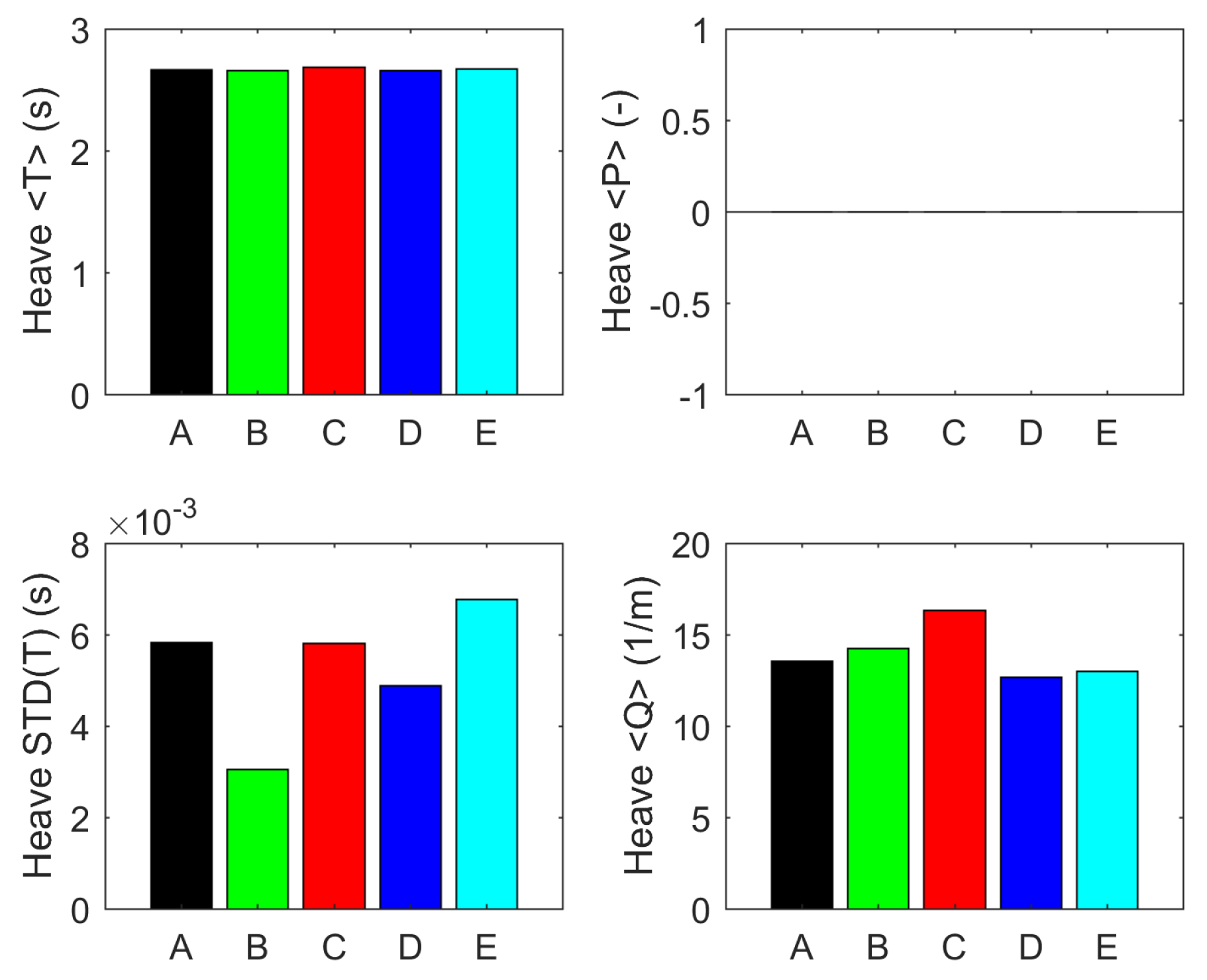
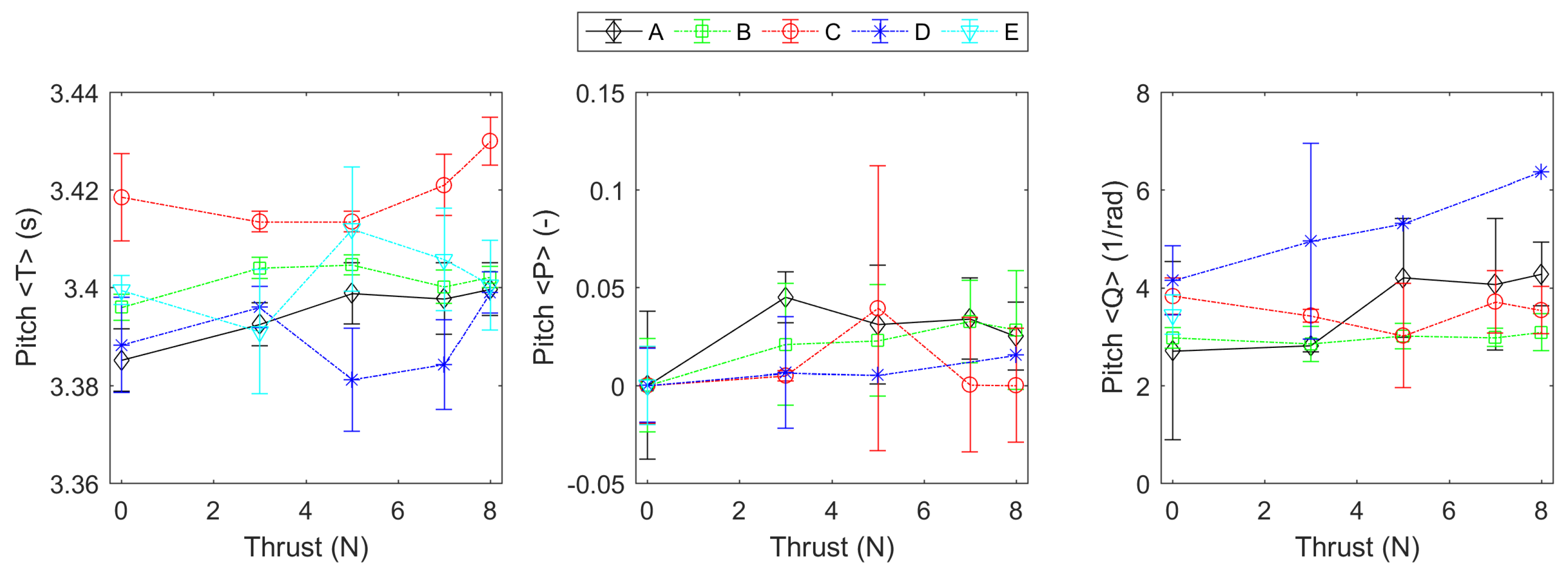
5.3. Still Water Decay Tests

Decay tests for the 6 DOFs of the moored system were completed in all basins. Additional decay tests were performed at certain facilities without the thruster power cables attached.

The first objective of a decay test is to measure the natural period of the motion mode which is predominantly responding to the position offset. The second objective is to assess the nature of the damping and quantify it. For the purposes of comparing the results of extinction tests across all facilities, the tests were analysed in the same way, according to the “PQ analysis method” presented by Vegt [12]. The method derives the estimates for the natural period, the linear and quadratic components of the damping in the form of two coefficients P and Q: P represents the linear damping and Q represents the quadratic damping. This method deals with only one DOF at a time. It should be noted that this method loses robustness when the main decay is affected by peripheral noise such as contributions of other DOFs induced by coupling. A variable number of decays were run in each basin. Even if a few decays were not exploitable by the PQ analysis, most of them could be used. For each test set-up, the averages of the exploitable test results are presented in this paper. The left column of Figure 6 contains the average of the surge period and its associated standard deviation. The right column shows the averages of the linear damping P (top) and the quadratic damping Q (bottom). Figure 7 presents the results for heave, and Figure 8 for pitch.

For surge, most of the periods are in the range of 19 s–20 s. The surge period of D is much shorter than the surge periods of the other campaigns. This is consistent with the main observation made during the analysis of the global stiffness across all facilities: the mooring system of D is significantly stiffer than the others. $B_0$ and $D_0$ are used to indicate that these results were done without the power cable whereas the power cable was installed in B and D. In both cases, the surge period is slightly shorter with the power cable than without. This confirms the hypothesis that the power cable is stiffening the mooring system, discussed in Section 6.1. The surge period for E is somewhat of an outlier (Figure 6). However, few decay tests could be used for E and the average period may not be representative of the best decay motion as it is reflected by the large standard deviation.

In the right column of Figure 6, the averages of the quadratic damping coefficients Q are much bigger and more consistent than the averages of the linear damping coefficients P. This indicates that the quadratic damping is dominant. Although the standard deviations of Q for each model-testing set-up are not displayed, they were comparable with the variations of the averages between facilities.

The averaged heave periods are the same across all facilities (left column of Figure 7). The standard deviation of the heave periods is close to zero for every basin. The damping in heave is fully quadratic (right column of Figure 7). The pitch period is also identical for all basins (Figure 8). The periods derived from repeated tests are very consistent for most facilities. The damping in pitch is also fully quadratic.

The decay results for other DOFs will be examined in a separate paper, however, the main observations are briefly outlined here. For all basins except D, the sway decay periods were found to be very close to the surge natural periods measured with the same test set-up. For D, the sway period was much larger than the surge period shown in Figure 6. This exhibits a strong asymmetry in the mooring system of D. The roll periods were very similar to the pitch periods for all testing set-ups. Significant variations were observed between facilities for the natural periods in yaw.

Decay tests were also performed in still water while the propeller was active. This was done for 4 levels of thrust: 3N, 5N, 7 and 8N. Decays in surge and pitch were analysed following the same approach as the extinction test without thrust. For each level of thrust (starting with T = 0 N), the average period, the linear damping coefficient P and the quadratic coefficient Q were determined utilising the PQ analysis. For several campaigns, multiple decay events could not be properly analysed. Therefore, the averages of the results are plotted and not the results of all individual decay events. For every level of thrust, the average period is displayed with an error bar. The length of this error bar corresponds to 2 times the standard deviation associated with all decay events analysed for this thrust during this particular campaign. Figure 9 presents the results for surge, and Figure 10 those for pitch. These figures show that the surge period is impacted more by the thrust than the pitch period. 3 out of 5 campaigns exhibit a slight decrease of the surge period with increasing thrust, whereas the surge period is stable in one campaign and slightly increasing in the last campaign. It is noted that the effect of the power cable on the surge period is of the same order as the variation of the surge period under different levels of thrust (Figure 6).

5.4. Responses in Waves

Tests in regular and irregular waves were completed by all facilities. This research focuses on the irregular waves; a detailed regular wave analysis will be presented in future publications.

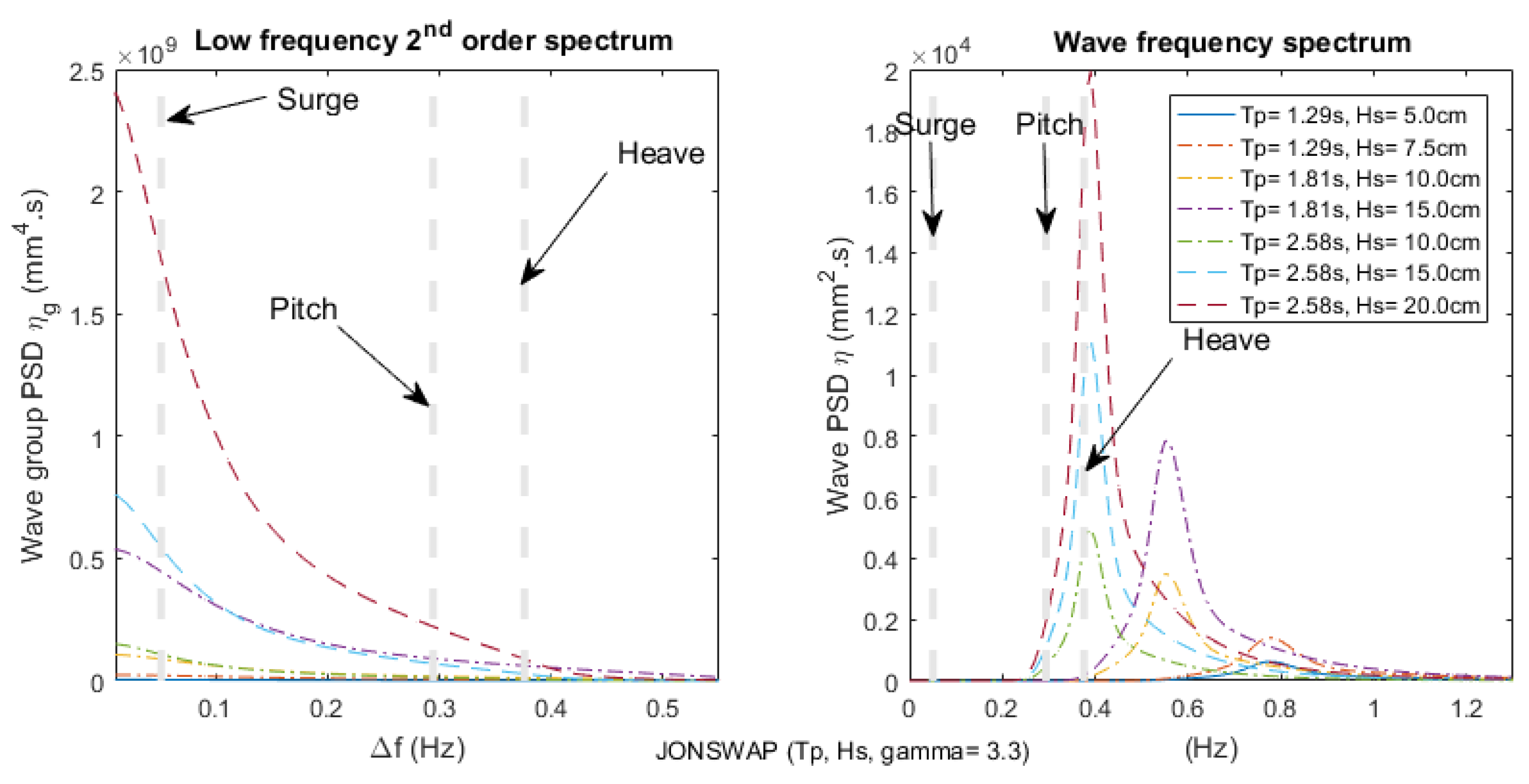
5.4.1. JONSWAP Waves and Expected Effects on Responses

As described in Table 3, 7 irregular waves were run in all facilities characterised by JONSWAP spectra with 3 distinct periods and a variety of wave heights. The right hand plot of Figure 11 shows the theoretical power spectral densities (PSDs) of the tested waves. It illustrates in which frequency range the responses to each wave train can be expected. A total range of [0.2, 1.2] (Hz) is covered by these waves. Under the linear assumption, the whole response of the system should be limited to this range. Nevertheless, any floating system is also likely to move at its natural periods. As presented in Section 5.3, the resonance frequencies of the studied submersible are all located below 1.2 Hz. Therefore, only frequencies below this figure are considered for resonance responses. The left hand plot of Figure 11 shows the second order difference frequency spectra which can be deduced by applying the following quadratic operator ($S_{\eta }^2$) to each JONSWAP spectrum:

$$S_{\eta }^2(\Delta f)={\int }_{f_1}^{f_2}{S}_{\eta }\left(f\right)S_{\eta }(f+\Delta f)df,$$

(1)

where $\eta$ is the wave elevation, $S_{\eta }$ is the wave spectrum and $[f_1$, $f_2]$ is the wave frequency range.

For a given wave spectrum, this operator sums the product of the 2 amplitudes of all combinations of bi-chromatic waves with the same difference frequency. The values of the difference frequency are given in the x-axis. As the difference between the two frequencies of a bi-chromatic wave is equal to the frequency of its envelope, the second-order difference frequency spectrum is also called the “wave envelope spectrum” or “wave group spectrum”. Figure 11 illustrates which low frequencies can be excited by a quadratic response to the 7 irregular waves. The eigen frequencies of the surge, heave and pitch motions are drawn with dashed vertical grey lines on both plots in Figure 11 and indicate when resonance is expected to occur for any of these modes. The right hand side of Figure 11 shows that the surge eigen frequency lies outside the range of all the JONSWAP wave spectra. The pitch and heave eigen frequencies fall within the wave frequency range of the JONSWAP waves with a peak period of 2.58 s. The pitch eigen frequency lies just within the range of the JONSWAP waves with peak period of 1.81 s. The left plot of Figure 11 shows that the surge eigen frequency should be the most impacted by the second order difference frequency spectra. The eigen frequencies of pitch and heave are decreasingly affected by the wave group spectra.

Table 5. Resonance response type per wave condition (LF = Low frequency; WF = Wave frequency).

Motion Mode	Surge	Heave	Pitch
JONSWAP $T_p=1.29$ s	LF	LF	LF
JONSWAP $T_p=1.81$ s	LF	WF	LF
JONSWAP $T_p=2.58$ s	LF	WF	WF
Pink-Noise	LF	WF	WF

records the nature of the responses that can be expected per motion DOF for each JONSWAP wave. Here, LF refers to ‘low frequency’, i.e., frequencies below the range of the associated JONSWAP spectrum, i.e., the wave frequency, WF. The wide spread of amplitudes in the right hand plot of Figure 11 illustrates how diverse the response levels in the wave frequency range can be for the 7 waves. However, as long as these responses are linear with the wave height, results for these 7 waves can be compared using spectral Response Amplitude Operators (RAO), as defined in Equation (2). For the low frequency range in the graphic on the left, the spread between the amplitudes of the curves is very large. In this frequency range, RAOs are useless and another kind of operator needs to be found for the comparison of low frequency responses.

$$RAO=\sqrt{\frac{S_{signal}}{S_{\eta }}}$$

(2)

where $S_{\eta }$ is the wave spectrum and $S_{signal}$ is the power spectral density of the considered signal. Both spectra are calculated on the same frequency range $[f_1$, $f_2]$.

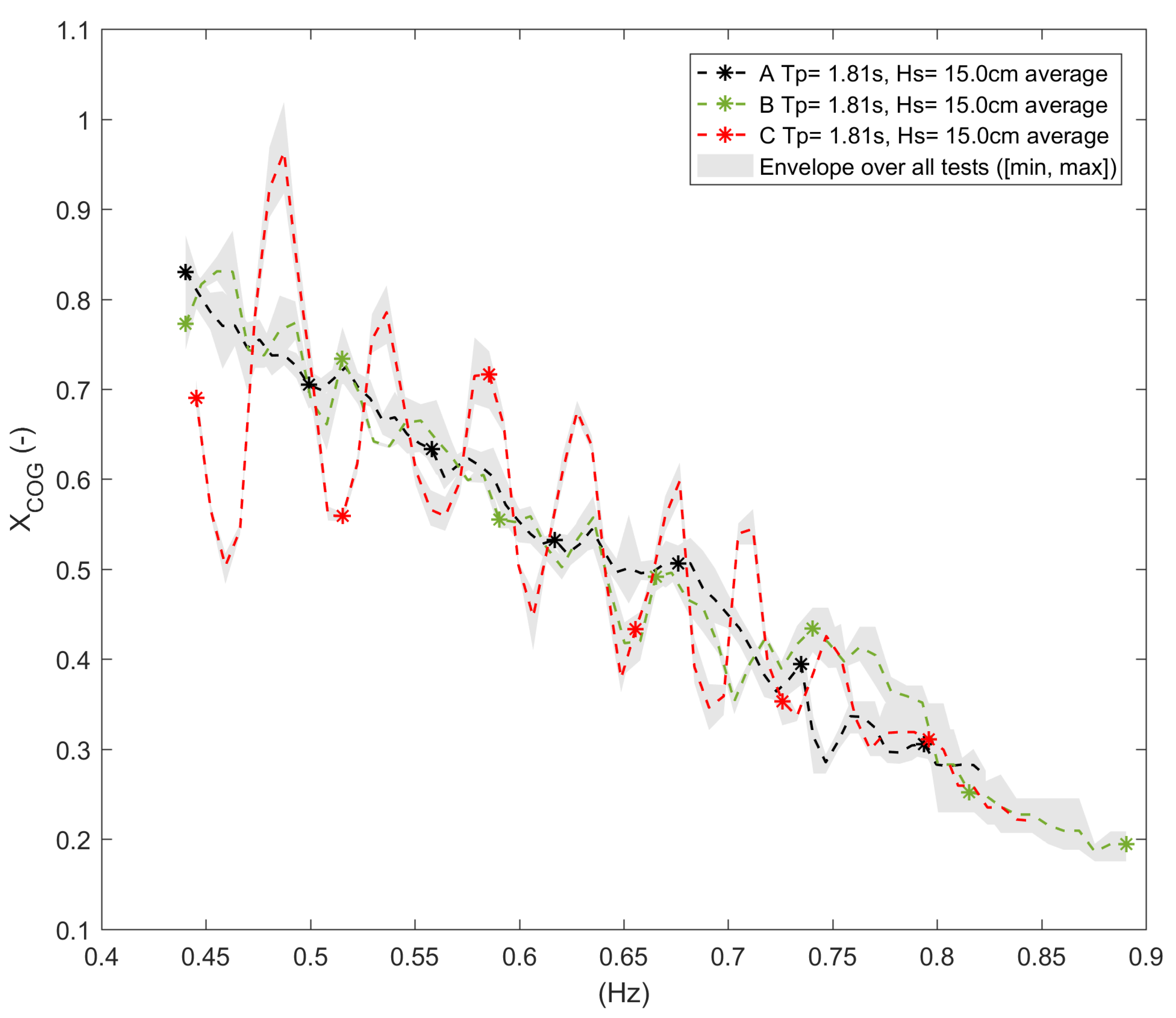
5.4.2. Effect of Wave Seed on Responses

Irregular waves are generated in a wave basin by combining a number of linear wave components. The phases associated with the wave components are pseudo-random in that a random number generator is used to assign the phases, but by using the same seed, the wave train obtained will be the same each time. Random effects in the wave train can be introduced by generating waves with the same target spectrum but distinct seeds. This has been done for JONSWAP $T_p=1.81$ s and $H_s=15$ cm in 3 basins. 5 seeds were used in A while 3 were used in B and C. One seed was used in the tests carried out in D. This wave was not tested in E. The results of basins A, B and C for JONSWAP $T_p=1.81$ s and $H_s=15$ cm are used to investigate the effect of the wave seed on the motion responses.

For each facility, the average RAO is presented together with its envelope (minimum and maximum) in Figure 12, Figure 13 and Figure 14. Figure 12 shows the surge RAOs for the 3 basins. Figure 13 displays the heave RAOs, and Figure 14 shows the pitch RAOs. For each basin, the envelopes illustrate the variation in the RAOs introduced by the use of several wave seeds. The differences between basins are bigger than the differences between RAOs obtained from waves with distinct seeds in the same basin. The RAOs of some basins oscillate around the RAOs of the others. This is most apparent in the surge RAO of C (Figure 12), but it can also be observed for the heave RAOs of B and A (Figure 13), and for the pitch RAOs of B and C (Figure 14). These oscillations stay present for all seeds. It can be concluded that these oscillations are not random but specific to each basin. Reflection of the incoming waves is suspected to be the main cause behind these oscillations. This is discussed in Section 5.4.4.

The deviations in $H_s$ and $T_p$ of the realised wave trains with different seeds for basins A, B, and C are presented in

Table 6. Variations in $H_s$ and $T_p$ for different random seed tests.

(Max-Min)/Mean (%)	A	B	C	A+B+C
$H_s$	4.0	9.0	2.2	26.3
$T_p$	1.0	2.1	1.4	3.6

. The last column of Table 6 presents the deviations when results of the 3 basins are considered together. It can be seen that $H_s$ varies significantly more than $T_p$ with the seed. The deviation of $H_s$ between facilities is large. However, it should be stressed that there was no specific agreement between facilities on the wave calibration process. Therefore, the duration of the wave and the frequency range on which the target wave spectrum is replicated by the wave makers were not the identical in these basins. These differences can explained the large deviation in the last column of Table 6.

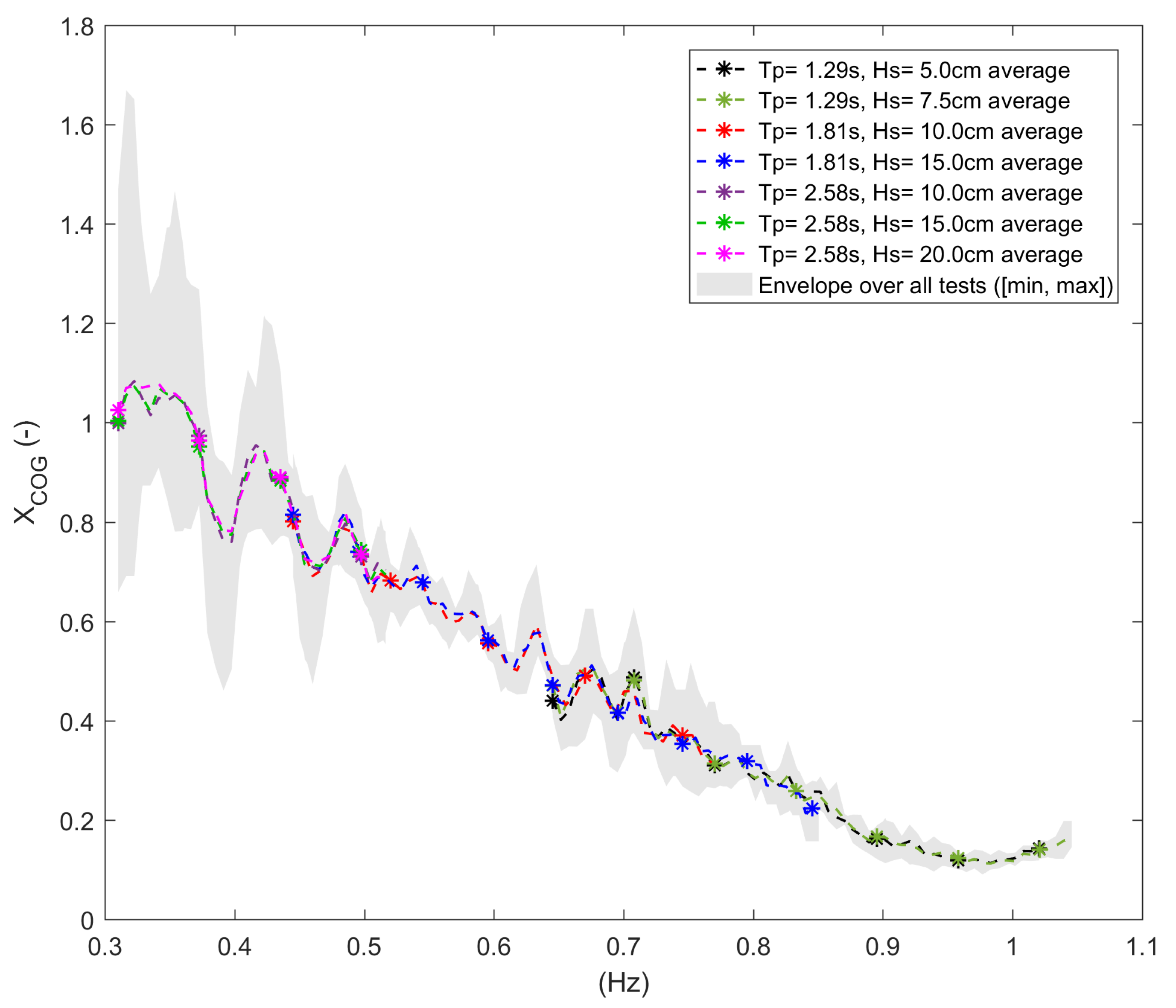
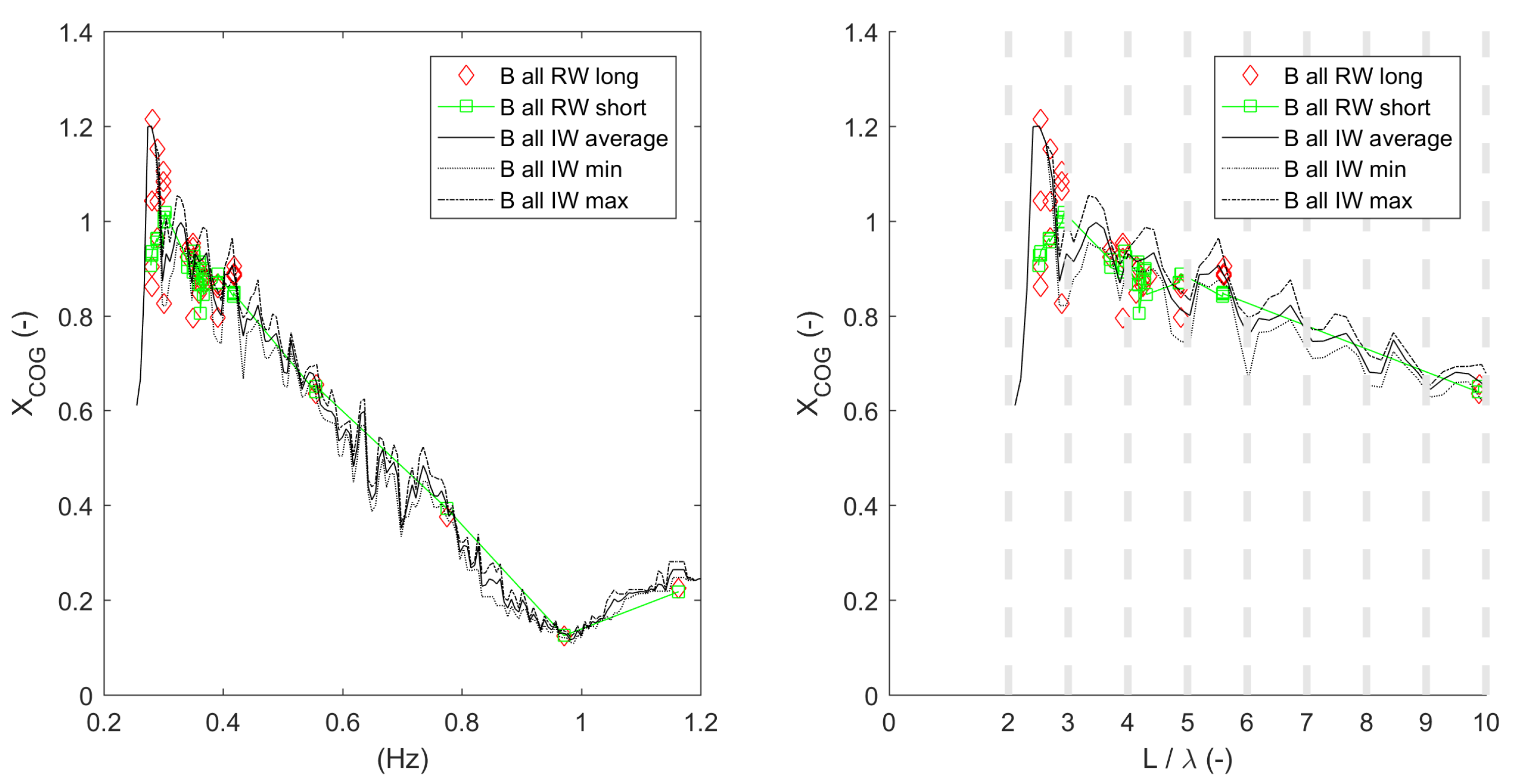
5.4.3. RAOs for All JONSWAP Waves

Figure 15, Figure 16 and Figure 17 display the average RAOs for all the JONSWAPs considered. The “average” is determined by taking the average of the RAOs obtained from all basins for a specific JONSWAP wave. Each average RAO is surrounded by its envelope in shaded in grey, allowing the visualisation of both global trends and the spread in the results between facilities. Figure 15, Figure 16 and Figure 17 show that the results obtained from all facilities lead to the same global RAOs but sometimes with important variations. Each RAO is discussed separately in this section.

The variations in the surge RAO are amplified as the frequency decreases (Figure 15). For all facilities, the surge RAOs exhibit oscillations in the 0.3 Hz to 0.5 Hz range. These oscillations are not equally big for all facilities and largely disappear at higher frequencies (above 0.8 Hz).

The agreement between facilities is strongest for the heave RAOs (Figure 16) (as it can be judged by the relatively narrow envelopes). The spread in results is small for frequencies above 0.5 Hz. The RAOs of all basins capture the resonance peak (0.37 Hz) and the heave cancellation frequency (0.43 Hz) at the same frequencies. The variation of the RAO amplitudes is most pronounced around these two frequencies. Looking specifically at the heave responses for JONSWAP $T_p=2.58$ s for different $H_s$ (i.e., the purple, green and pink lines in Figure 16), it can be seen that the resonance peak decreases as the wave height increases. The trough at the cancellation frequency is less deep for bigger $H_s$. For a specific targeted spectrum with identical $H_s$, the spread between facilities is significant. It has been observed for all irregular waves that waves are different between basins even though the target spectrum and $H_s$ are the same. This combined with the sensitivity of the resonance peak to $H_s$ explains the larger spread in the RAOs from different basins around the eigen frequency in heave. The same can be said for the trough at the cancellation frequency.

The pitch RAOs are very similar across all facilities (Figure 17). The prediction envelope is broader in the [0.3, 0.45] (Hz) range than for higher frequencies. The starting frequency of 0.3 Hz is close to the pitch eigen frequency (0.29 Hz) and the effect of the wave height is strong at this frequency. In the same way as for heave, the pitch response peak decreases with increasing $H_s$. As for heave, differences in achieved $H_s$ between facilities for the same target wave (JONSWAP $Tp=2.58$ s) lead to large discrepancies between RAOs close to the pitch resonance peak.

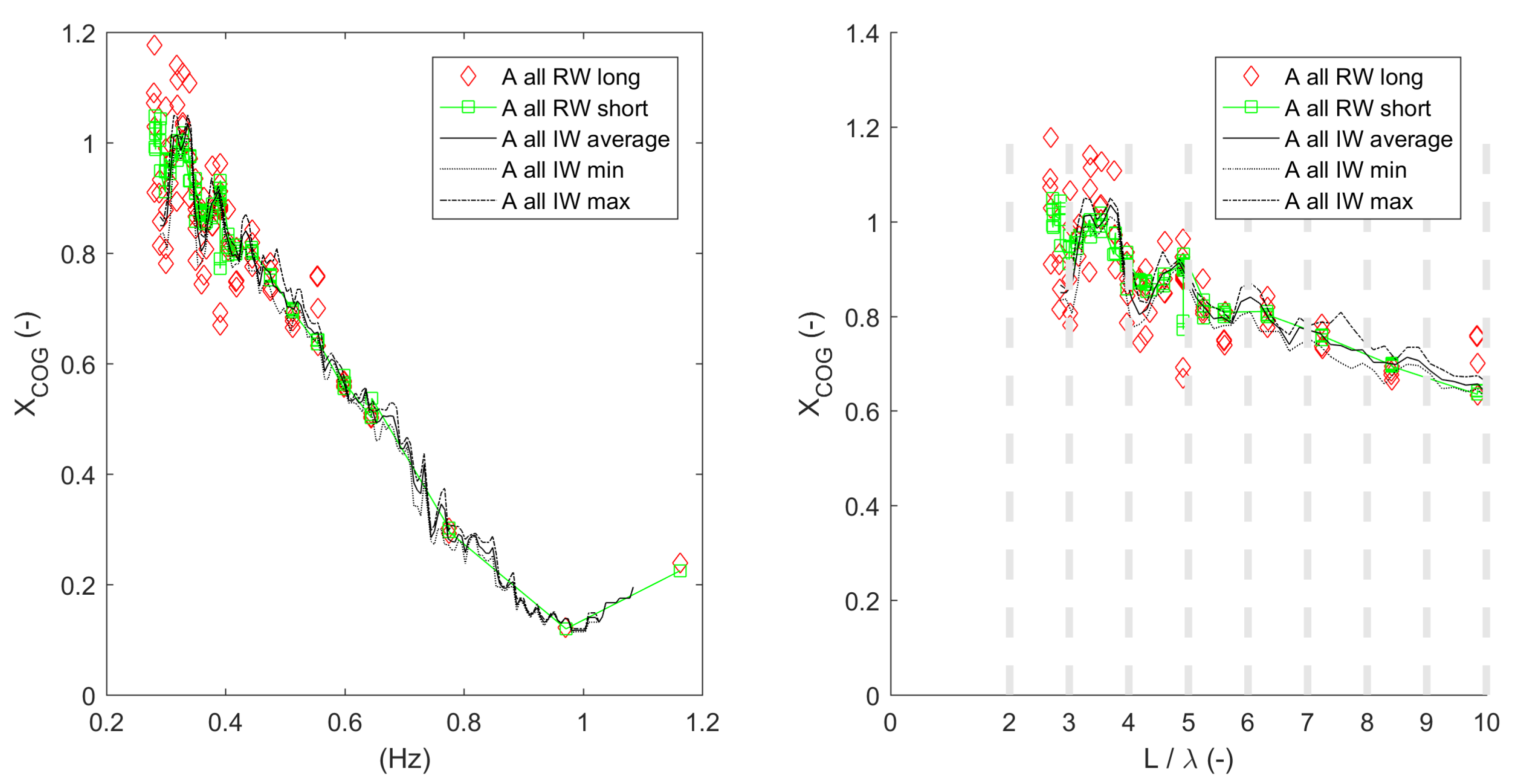
5.4.4. Impact of Reflection

Basins are generally designed to limit reflections by incorporating an absorbing beach and sometimes through active reflection compensation at the wave maker. However, it is not possible to eliminate reflections completely. Waves whose wave lengths are multiples of one dimension of the basin are particularly troublesome [13].

A regular wave test is commonly used to obtain the responses of the floater at the single frequency of the generated wave. The list of tests in regular waves carried out in all basins in the RR campaign are listed in (Table 2). Conveniently, it is relatively easy to assess the effect of reflection for a test in regular waves. From the moment that the wave reaches the model, it takes time for the longitudinal wave to reflect off the end of the basin and return to the model. This delay can be estimated by dividing the total distance that the wave needs to travel by the group velocity. The time delay is a good opportunity to look at the responses of the floater in the two situations: without and with longitudinal reflection. In practice, two different time intervals of the same wave test are analysed: one before the longitudinal reflected wave is present; the other after the longitudinal wave has arrived at the model location. Generally, avoiding or minimising reflection leads to the selection of a much shorter interval than when reflections are accepted. Therefore, the interval attempting to minimise reflection is labelled ‘short’ in this section. This approach is explained and applied to the test results of a wave energy converter in [8]. For regular waves, the ratio of the amplitude of the 1st harmonic of a signal by the 1st harmonic of wave elevation gives the RAO coefficient for the wave frequency as detailed in Equation (3).

$$RA{O}_{reg}=\frac{a_{signal}^{\left(1\right)}}{a_{\eta }^{\left(1\right)}}$$

(3)

where $a_{\eta }^{\left(1\right)}$ is the amplitude of 1st harmonic of the wave elevation and $a_{signal}^{\left(1\right)}$ is the amplitude of 1st harmonic of the considered signal. By combining the results from all regular wave tests, RAOs can be obtained and compared to those of irregular wave tests which most likely include some effects of reflection. This has been done for the surge, heave and pitch motions but only the surge RAOs are presented here as large oscillations have been noticed in these RAOs for some basins. The results for heave and pitch were reasonably consistent across the basins. The following RAO data are shown for the four basins in Figure 18, Figure 19, Figure 20 and Figure 21:

• ‘Short’: RAO obtained from all regular waves using time intervals during which the longitudinal reflected waves have not yet reached the model. As the wave periods get longer, the wave travels faster and this interval becomes shorter.
• ‘Long’: RAO obtained from all regular waves using a time interval that includes the effect of the longitudinal reflected waves. This interval is chosen so as to be as long as possible, and aims to capture a sequence of wave cycles during which the wave is fully developed and the motions are steady.
• ‘IW’: average RAO and its envelop obtained from all tests with irregular waves in the basin (i.e., JONSWAP and Pink-Noise waves when available). These results include the effects of the reflected waves.

The surge RAOs are displayed as a function of the wave frequency (in Hz) and $L/\lambda$, i.e., the basin’s length divided by the wave length. For a given regular wave, this ratio is different for every basin as it varies with the basin’s length (L) and the water depth which comes into play for the determination of the wave length ($\lambda$). This on its own explains why the level of reflection is intrinsic to each basin. Moreover, every basin has its own tools to limit the reflection like a beach or the compensation algorithm that controls the paddles of the wave maker. The RAOs are plotted for the 4 basins as follows: A (Figure 18), B (Figure 19), C (Figure 20), and D (Figure 21).

The RAOs determined from the regular waves agree globally with the average RAOs obtained from irregular waves (Figure 18, Figure 19, Figure 20 and Figure 21). Nevertheless, the dispersion of the RAO data points along the vertical axis is more pronounced for the regular wave RAOs (e.g., the red and green circles on the the left hand plot of Figure 18). This dispersion is larger when long intervals are used rather than short intervals for every frequency below 0.6 Hz in all basins (red circles compared to green circles on Figure 18, Figure 19, Figure 20 and Figure 21). This confirms that longitudinal reflection is a major contributor to the dispersion of the RAO coefficients for long periods. The right hand plots in Figure 20 and Figure 21 show that large dispersions coincide with the basin length being a multiple of the wave length (i.e., the circles are aligned with the dashed grey lines). This is true for RAOs calculated from tests in regular and irregular waves. Sometimes the basin length is not a multiple of the wave length for frequencies with large dispersion of the RAO coefficients for long periods (e.g., Figure 18 and Figure 19). For these cases, other explanations must be sought (e.g., transverse reflections, testing durations too short for an accurate analysis with long intervals).

The RAOs calculated from the tests in regular waves show an important spread (e.g., Figure 18, Figure 19, Figure 20 and Figure 21). This spread is acute for waves with the longest periods. As these waves were generated for several wave amplitudes (Table 2), this spread illustrates the non-linear behavior of the surge response below 0.4 Hz. A similar spread was observed in the plot of all results of irregular wave tests (Figure 15) which also included several wave amplitudes.

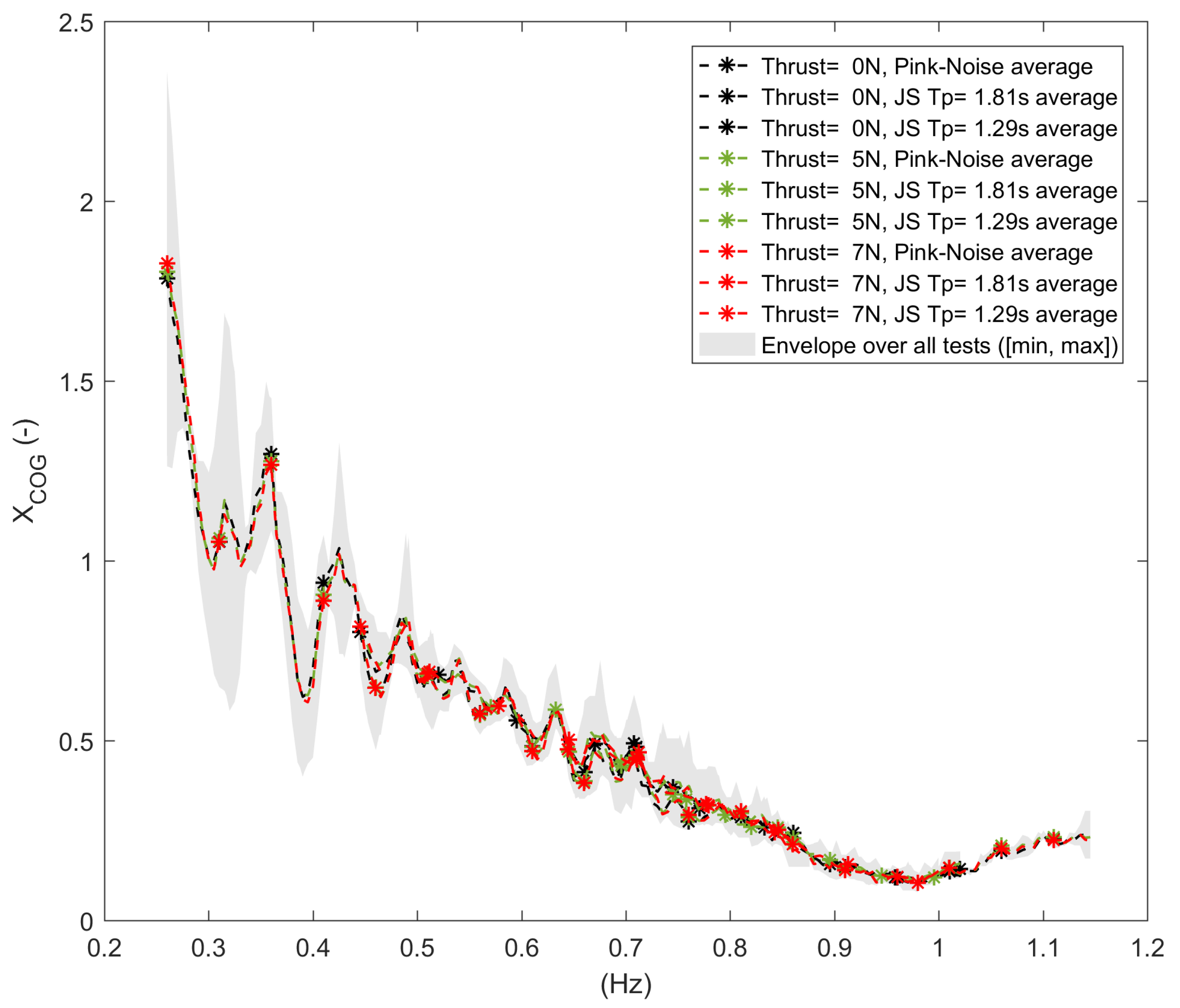
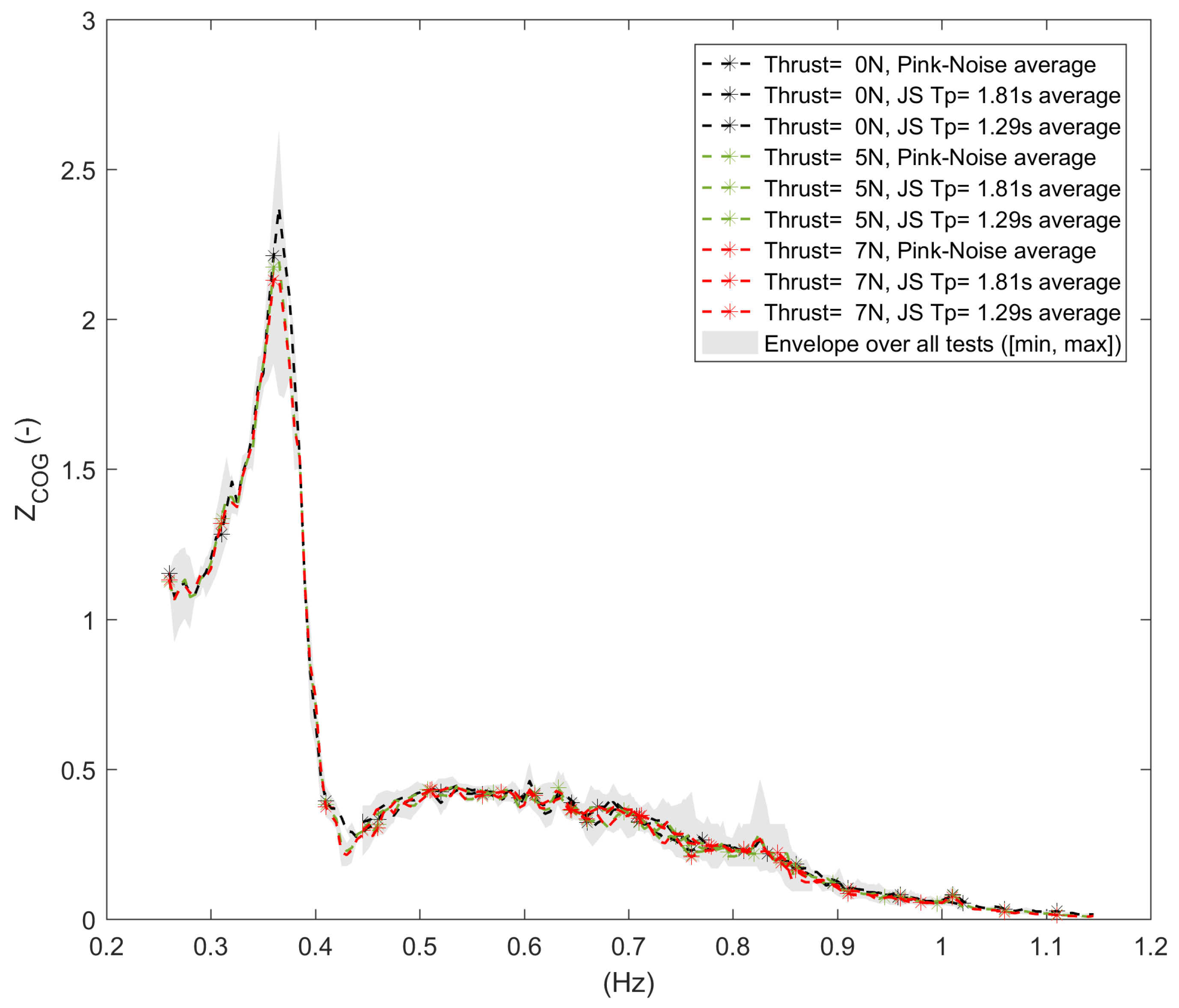
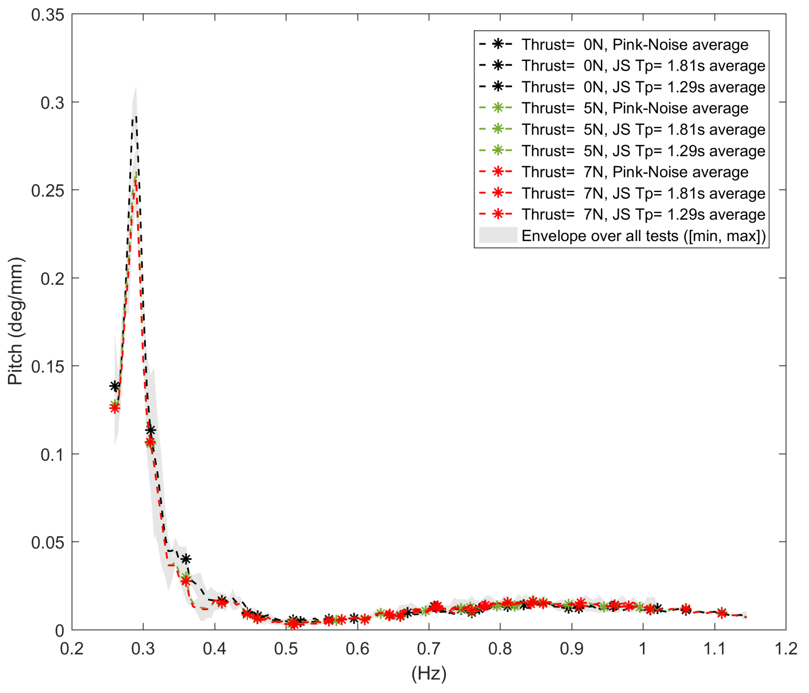
5.5. Responses in Waves under Constant Thrust

Tests in irregular waves with the thruster in operation were completed as outlined in Table 3. Most facilities completed tests involving JONSWAP spectra for two peak periods and some variations of significant wave height with constant thrust of 5N and 7 N. Additionally, Pink-Noise waves were tested in combination with constant thrust in two basins. One basin (D) tested the system in the longest wave (JONSWAP $Tp=2.58$ s) in combination with constant thrust. The motion RAOs are examined and then their evolution under the effect of the thrust are compared. This is done for at least three levels of thrust (0 N, 5 N and 7 N) plus additional levels when the data are available.

The average RAOs over all facilities and the associated envelope defined by the minimum and maximum values are plotted in Figure 22, Figure 23 and Figure 24. The black lines and markers represent RAOs with no thrust, green corresponds to a thrust of 5 N and red corresponds to 7N. Noticeable variations in the average surge RAOs due to thrust are not observed (Figure 22). The resonance peak of the heave RAOs (Figure 23) is observed to decrease with higher thrust but this decrease is small and within the level of variation of the RAO between the 4 basins. The resonance peak in pitch (Figure 24) also reduces with increasing thrust. When the thrust is set to 5 N (from 0 N), this drop is significant and out of the envelope of variation of the RAOs over the 4 facilities. However, the decrease is much smaller when the thrust increases from 5 N to 7 N. Outside the resonance peaks, the RAOs in heave and pitch are not significantly impacted by the thrust.

6. Discussion

The same floating wind turbine model was tested five times at the same scale in four distinct facilities, with some minor differences between test set-ups (especially in the mooring anchor positions for facility D). It has been found that most of the results obtained are very comparable across facilities. However, there are differences too. Some of these differences are believed to be inevitable with current state of the art model-testing techniques. These variations and their impacts are discussed in this section.

6.1. Global Surge Stiffness

The characteristics of the mooring system and the main elements required to assemble it (i.e., the springs and mooring lines) were provided to all basins. However, the mooring system had to be implemented in 4 basins with major size differences. For the narrowest basin, the mooring lines on port and starboard had to be installed with a much narrower azimuth angle between them in order to fit (Table 4). This resulted in a surge stiffness for this facility which was 2/3rd greater than for the other facilities. For the three other basins, the anchor points may not have been located precisely at the same positions in each facility. The stiffness in surge shows variations of the order of 1/10th for the basins that used the same azimuth angle for the two side lines (Table 4).

The disturbance caused by the power cable has been reported multiple times in literature covering the model-testing of FOWTs [14]. In the present round robin campaign, the positioning of the cable and how it was supported was inevitably different in each facility, causing different levels of interference. The level of interference may also have changed within the course of a campaign through being re-arranged or its lay-out inadvertently modified when large excursions of the model occurred. The results indicate that the power cable caused differences in the surge stiffness and the surge natural period of the model. It was observed (Figure 9) that the surge period changed under the effect of thrust (4%). Moreover, this change was not the same for all campaigns. Discrepancies in the global surge stiffness affects the surge period. As a consequence, the frequency coinciding with the surge resonance peak is not consistent between all tests in waves. The resonance peaks of the mooring line tensions were equally affected by the discrepancies in the surge stiffness as surge was the main drift mode in this test campaign. It can therefore be stated that the surge stiffness is the main source of uncertainty for this experimental set-up. It is difficult to determine how big the impact of the power cable on the global surge stiffness is as it most likely varies with the experimental conditions (decay tests, tests in waves, and tests in wind).

6.2. Damping

The nature of the damping for surge, heave and pitch motions was similar in all test campaigns (Section 5.3). The damping is mainly quadratic for surge with a small linear contribution. It is very dominantly quadratic for heave and pitch. This shows that the viscous loads on the columns and the pontoons are much larger than the wave radiation damping for these motions. Significant variations were observed on the estimated damping coefficients between test campaigns.

The way the decay motion was initiated (and especially the starting amplitude) is suspected to have a large influence on this evaluation. In some instances, access to the model was difficult, due to the distance between the model and the carriage or the side walls. In some basins, the operators could push or pull the model directly while standing outside the basin. Others had to do so while on board a small barge adjacent to the model. The starting amplitudes of the decays are different in all decay tests. As reported by [15], the damping can vary with the amplitude of the initial offset.

As noted in the previous section, the power cable is noted as a source of discrepancies between the campaigns. Although the effect of the cable on the estimation of the damping coefficients was noticeable, it was of the same order as the variations between facilities.

No significant effect of the propeller’s thrust on the aerodynamic damping could be found from the decay tests under constant thrust. The aerodynamic damping that can be expected from a wind turbine in operation [16,17] is not reproduced by this system. If the thrust has an impact on the surge period then this effect is not identical across all campaigns. When the model moves to a new equilibrium position under the effect of the constant thrust, the interaction of the power cable and the model is likely to change. This might mask or amplify the evolution of the surge period under the effect of the thrust.

6.3. Wave Height and Wave Steepness with the Interference of Reflection

The disparity between the realised wave heights in all basins was significant despite common wave specifications. The variation of the realised values of wave steepness across all basins for the same target wave was also important. This was witnessed both for regular and irregular waves.

The processes by which waves are generated and calibrated are not the same for all facilities. Furthermore, the dimensions of the four basins are very different. They vary from a long and narrow basin to more square shaped basins. The deepest basin is almost 4 times deeper than the shallowest basin. Each basin is equipped with at least a beach opposite the wave maker to passively absorb energy by wave breaking, but each beach has different characteristics. In addition, the wave maker devices are also different (piston wave maker in one facility and hinged paddles in the others). Moreover, the software steering the wave maker is sometimes fundamentally different. Some basins are equipped with wave makers that include active wave absorption, whereas others are not.

Due to these differences, the wave reflection level and how it is dealt with is not the same across all basins. Some frequencies are more or less affected by wave reflection depending on the dimensions of the basins. The differences between surge responses in different facilities testify to that (see how broad the envelope is in Figure 15). Wave reflection is thought to be behind the large oscillations observed in the surge RAOs for frequencies below 0.6 Hz throughout all kinds of tests with waves (Figure 12, Figure 15 and Figure 22). In addition, the wave height in every basin is affected by random uncertainty, as evidenced in Table 6.

Differences in wave height at the location of the model are not an issue as long as all the responses of the tested specimen are linear. RAOs can then be determined for each test and facility allowing a fair comparison within the wave frequency range. However, differences in wave height represent a real challenge when responses stop being dominantly linear. This is the case for all responses of this semi-submersible platform around their natural periods (Table 5). At resonance, the surge response in waves reacts to non-linear wave drift loads for all wave conditions. At the heave resonance frequency, viscous loads on the bottom of the columns and the pontoons are non-linear. Similarly, these loads become important for large pitch rotations (i.e., around the pitch resonance frequency). For some irregular waves (Table 5), the pitch and even the heave motions react to higher order difference frequency wave loading. The above explains why the motion responses to waves vary with the wave height around the resonance frequency for surge, heave and pitch. This dependency hinders direct comparison of RAOs obtained from basins where the wave heights were not equal. The work-around followed in this study has been to look at the evolution of RAOs while some test parameters are varied. The trends in the evolution of the RAOs with regard to the variation of the wave height have been compared for the four basins. This has been done for tests in waves while constant thrust was applied to the model.

For tests with increasing wave height, the trends observed in the evolution of the RAOs were the same in the four basins. The RAOs were stable as long as the wave frequency range did not include any of the resonance frequencies in heave and pitch (JONSWAP $T_p=1.29$ s and $T_p=1.81$ s). The RAOs changed significantly with the wave height for the JONSWAP wave with $T_p=2.58$ s, the frequency range of which covered the heave and the pitch eigen frequencies. This indicates that the viscous loads were counteracting the wave excitation loads for these waves. As a result, the heave and pitch resonance response peaks experienced increased damping when the wave height increased (Figure 16 and Figure 17).

From the three investigated motions, the surge motion was found to be the most troublesome quantity for the cross facility comparison. It has been shown that its amplitude was heavily impacted by wave reflection at diverse levels across the four basins (Section 5.4.4).

6.4. Constant Thrust

For tests with increasing levels of thrust, the trends observed in the evolution of the RAOs were the same in the four basins. The effects of the thrust on the heave and pitch RAOs were mild for all wave conditions. The impact of the thrust was most significant on the pitch. The pitch resonance peak decreased under the effect of the thrust (Figure 24).

7. Conclusions

This article presents a round robin test campaign of a 1/60th scale semi-submersible floating wind turbine conducted in four basins with very different characteristics.

The linearity of the tested system has been explored in each basin. The global stiffness characteristics in surge, heave and pitch were found to be linear. For heave and pitch, they were equivalent for all facilities. The results in surge were mostly equivalent except for in one facility with a different mooring line arrangement which impacted the resonance response frequency for surge and the mooring line tensions. The effect on the power cable setup on the system varied between facilities with a small impact on the surge stiffness observed. The damping was not linear but mainly quadratic in all facilities, and was not affected by the thrust. The responses in waves were roughly equivalent for all facilities except for some discrepancies that could be explained. The responses in waves were linear with the wave height inside the wave frequency range excluding regions around the resonance and cancellation frequencies.

The wave generation was identified as a major source of discrepancies between facilities. Despite common target waves, the generated waves were different between basins. Reflection was found to be have a major impact on the surge motion, and the tensions in the mooring lines. The thrust did not significantly affect the responses in waves. Only the pitch resonance peak dropped under the effect of thrust when exposed to long waves. This effect was not linear and was observed in all basins. Wherever the response could be assumed to be linear, the RAOs of all basins agreed reasonably well once reflection is accounted for. For sea conditions and frequency ranges where it was expected that the responses would be non-linear, it was observed in all facilities. The quantification of these non-linear responses is left for further works.

This publication documenting the round robin campaign has primarily been concerned with checking how analog the results of the model-tests are and discussing their differences. The identification of the most relevant differences in the results is a first step; these differences will be explored further in future publications including the upcoming MaRINET2 deliverable “D2.5 Round robin findings and recommendations”.

References

1. Gueydon, S.; Bayati, I.; de Ridder, E.J. Discussion of solutions for basin model tests of FOWTs in combined waves and wind. Ocean Eng. 2020, 209, 107288. [Google Scholar] [CrossRef]
2. Noble, D.R.; Draycott, S.; Ordonez Sanchez, S.; Porter, K.; Johnstone, C.; Finch, S.; Judge, F.; Desmond, C.; Santos Varela, B.; Lopez Mendia, J.; et al. D2.1 Test Recommendations and Gap Analysis Report. Technical Report, MaRINET2. 2018. Available online: https://www.marinet2.eu/project-reports-2/ (accessed on 8 September 2021).
3. Noble, D.; O’Shea, M.; Judge, F.; Martinez, R.; Robles, E.; Corlay, Y.; Gabl, R.; Davey, T.; Vejayan, N. Standardising Marine Renewable Energy Testing: Gap Analysis and Recommendations for Development of Standards. J. Mar. Sci. Eng. 2021, 9, 971. [Google Scholar] [CrossRef]
4. Gaurier, B.; Germain, G.; Facq, J.V.; Johnstone, C.; Grant, A.; Day, A.; Nixon, E.; Di Felice, F.; Costanzo, M. Tidal energy “Round Robin” tests comparisons between towing tank and circulating tank results. Int. J. Mar. Energy 2015, 12, 87–109. [Google Scholar] [CrossRef] [Green Version]
5. Gaurier, B.; Ordonez-Sanchez, S.; Facq, J.V.; Germain, G.; Johnstone, C.; Martinez, R.; Salvatore, F.; Santic, I.; Davey, T.; Old, C.; et al. MaRINET2 Tidal Energy Round Robin Tests—Performance Comparison of a Horizontal Axis Turbine Subjected to Combined Wave and Current Conditions. J. Mar. Sci. Eng. 2020, 8, 463. [Google Scholar] [CrossRef]
6. Martinez, R.; Gaurier, B.; Ordonez-Sanchez, S.; Facq, J.V.; Germain, G.; Johnstone, C.; Santic, I.; Salvatore, F.; Davey, T.; Old, C.; et al. Tidal energy round robin tests: A comparison of flow measurements and turbine loading. J. Mar. Sci. Eng. 2021, 9, 425. [Google Scholar] [CrossRef]
7. Judge, F.M.; Lyden, E.; O’Shea, M.; Flannery, B.; Murphy, J. Uncertainty in Wave Basin Testing of a Fixed Oscillating Water Column Wave Energy Converter. ASCE-ASME J. Risk Uncertain. Eng. Syst. Part B Mech. Eng. 2021, 4, 040902. [Google Scholar] [CrossRef]
8. Ohana, J.; Gueydon, S.; Judge, F.; Haquin, S.; Weber, M.; Lyden, E.; Thiebaut, F.; O’Shea, M.; Murphy, J.; Davey, T.; et al. Round robin tests on a hinged raft wave energy converter. EWTEC 2021. [Google Scholar]
9. Gueydon, S. Effects of Variations on the Experimental Set-Up on the Motion Response of a Floating Wind Semisubmersible (OC4 Type). In Proceedings of the ASME 2019 2nd International Offshore Wind Technical Conference, St. Julian’s, Malta, 3–6 November 2019; Volume 59353, p. V001T01A020. [Google Scholar]
10. Sandner, F.; Wie, Y.; Matha, D.; Grela, E.; Azcona, J.; Munduate, X.; Voutsinas, S.; Natarajan, A. INNWIND.EU Deliverable 4.3.3—Innovative Concepts for Floating Structures. Technical Report. 2014. Available online: http://www.innwind.eu/publications/deliverable-reports (accessed on 8 September 2021).
11. Det Norske Veritas AS. DNV-RP-C205 Environmental Conditions and Environmental Loads; DNV GL: Høvik, Norway, 2014; Volume 15, p. 2018. Available online: https://rules.dnvgl.com/docs/pdf/DNV/codes/docs/2014-04/RP-C205.pdf (accessed on 8 September 2021).
12. Vegt, J.v.d. Slinger Gedrag van Schepen; KIVI-Lecture on seakeeping, Delft; 1984. [Google Scholar]
13. Newman, J.N. Analysis of wave generators and absorbers in basins. Appl. Ocean Res. 2010, 32, 71–82. [Google Scholar] [CrossRef] [Green Version]
14. Robertson, A.N.; Jonkman, J.M.; Goupee, A.J.; Coulling, A.J.; Prowell, I.; Browning, J.; Masciola, M.D.; Molta, P. Summary of conclusions and recommendations drawn from the DeepCwind scaled floating offshore wind system test campaign. In Proceedings of the ASME 2013 32nd International Conference on Ocean, Offshore and Arctic Engineering, Nantes, France, 9–14 June 2013; Volume 55423, p. V008T09A053. [Google Scholar]
15. Kvittem, M.I.; Berthelsen, P.A.; Eliassen, L.; Thys, M. Calibration of Hydrodynamic Coefficients for a Semi-Submersible 10 MW Wind Turbine. In Proceedings of the ASME 2018 37th International Conference on Ocean, Offshore and Arctic Engineering, Madrid, Spain, 17–22 June 2018. [Google Scholar] [CrossRef]
16. Bayati, I.; Facchinetti, A.; Fontanella, A.; Taruffi, F.; Belloli, M. Analysis of FOWT dynamics in 2-DOF hybrid HIL wind tunnel experiments. Ocean Eng. 2020, 195, 106717. [Google Scholar] [CrossRef]
17. Gueydon, S. Aerodynamic damping on a semisubmersible floating foundation for wind turbines. Energy Procedia 2016, 94, 367–378. [Google Scholar] [CrossRef] [Green Version]
18. Gueydon, S.; Lyden, E.; Judge, F.; O’Shea, M. MaRINET 2 Floating Offshore Wind Turbine Test Data Set—UCC; SEANOE, 2021. [Google Scholar] [CrossRef]
Figure 1. Model in the basin of Ifremer with the thruster.
Jmse 09 00988 g001
Figure 2. Layout and dimensions of the 1/60th scale model.
Jmse 09 00988 g002
Figure 3. Experimental setup in each facility.
Jmse 09 00988 g003
Figure 4. Photograph of a system of pulleys and wires designed for a static pull test.
Jmse 09 00988 g004
Figure 5. Surge and pitch offset (left), and surge ( K 11 ) and pitch ( K 55 ) stiffness coefficients (right).
Jmse 09 00988 g005
Figure 6. Surge natural periods (left), linear and quadratic damping estimates (right).
Jmse 09 00988 g006
Figure 7. Heave natural periods (left), linear and quadratic damping estimates (right).
Jmse 09 00988 g007
Figure 8. Pitch natural periods (left), linear and quadratic damping estimates (right).
Jmse 09 00988 g008
Figure 9. Effect of thrust on surge natural periods (left), linear (middle) and quadratic damping estimates (right).
Jmse 09 00988 g009
Figure 10. Effect of thrust on pitch natural periods (left), linear (middle) and quadratic damping estimates (right).
Jmse 09 00988 g010
Figure 11. Theoretical JONSWAP wave spectra (right) and the associated wave group spectra (left).
Jmse 09 00988 g011
Figure 12. Surge RAOs for all JONSWAP T p = 1.81 s H s = 15 cm waves with distinct seeds.
Jmse 09 00988 g012
Figure 13. Heave RAOs for all JONSWAP T p = 1.81 s H s = 15 cm waves with distinct seeds.
Jmse 09 00988 g013
Figure 14. Pitch RAOs for all JONSWAP T p = 1.81 s H s = 15 cm waves with distinct seeds.
Jmse 09 00988 g014
Figure 15. Surge RAOs for all JONSWAP waves: average and envelope (min and max).
Jmse 09 00988 g015
Figure 16. Heave RAOs for all JONSWAP waves: average and envelope (min and max).
Jmse 09 00988 g016
Figure 17. Pitch RAOs for all JONSWAP waves: average and envelope (min and max).
Jmse 09 00988 g017
Figure 18. Surge RAOs from regular and irregular waves in basin A (as function of frequency (left) and ratio of basin’s length by wave length (right).
Jmse 09 00988 g018
Figure 19. Surge RAOs from regular and irregular waves in basin B (as function of frequency (left) and ratio of basin’s length by wave length (right).
Jmse 09 00988 g019
Figure 20. Surge RAOs from regular and irregular waves in basin C (as function of frequency (left) and ratio of basin’s length by wave length (right).
Jmse 09 00988 g020
Figure 21. Surge RAOs from regular and irregular waves in basin D (as function of frequency (left) and ratio of basin’s length by wave length (right).
Jmse 09 00988 g021
Figure 22. Surge RAOs for all irregular waves: average and envelope (min and max).
Jmse 09 00988 g022
Figure 23. Heave RAOs for all irregular waves: average and envelop (min and max).
Jmse 09 00988 g023
Figure 24. Pitch RAOs for all irregular waves: average and envelop (min and max).
Jmse 09 00988 g024