
Short Word-Length Entering Compressive Sensing Domain: Improved Energy Efficiency in Wireless Sensor Networks


1
College of Engineering, University of Baghdad, Baghdad 10071, Iraq
2
School of Engineering, Edith Cowan University, Joondalup 6027, Australia
*
Author to whom correspondence should be addressed.
Information 2021, 12(10), 415; https://0-doi-org.brum.beds.ac.uk/10.3390/info12100415
Submission received: 30 August 2021
/
Revised: 8 October 2021
/
Accepted: 9 October 2021
/
Published: 11 October 2021
(This article belongs to the Special Issue Smart Systems for Information Processing in Sensor Networks)
Abstract
:This work combines compressive sensing and short word-length techniques to achieve localization and target tracking in wireless sensor networks with energy-efficient communication between the network anchors and the fusion center. Gradient descent localization is performed using time-of-arrival (TOA) data which are indicative of the distance between anchors and the target thereby achieving range-based localization. The short word-length techniques considered are delta modulation and sigma-delta modulation. The energy efficiency is due to the reduction of the data volume transmitted from anchors to the fusion center by employing any of the two delta modulation variants with compressive sensing techniques. Delta modulation allows the transmission of one bit per TOA sample. The communication energy efficiency is increased by RⱮ, R ≥ 1, where R is the sample reduction ratio of compressive sensing, and Ɱ is the number of bits originally present in a TOA-sample word. It is found that the localization system involving sigma-delta modulation has a superior performance to that using delta-modulation or pure compressive sampling alone, in terms of both energy efficiency and localization error in the presence of TOA measurement noise and transmission noise, owing to the noise shaping property of sigma-delta modulation.
1. Introduction
The vast advances made in wireless technology and electronics have enabled the emergence of wireless sensor networks (WSN) which have received much attention recently and are expected to become commonplace due to playing a major role in various applications such as industrial monitoring, health care monitoring, environmental sensing, target tracking, etc. Since sensors are usually small low-power devices powered by batteries that have limited lifetime, they are usually designed to send data to a fusion center at which most of the energy-consuming computations are performed. An example of data sent to the fusion center for processing are the time-of-arrival (TOA) samples needed for range-based anchor-based localization, which is the application considered in this work. The TOA data obtained at the anchors and sent to the fusion center for processing are indicative of the distance between an anchor and the target sensor to be localized or tracked. However, data processing is not the only energy-consuming process encountered. In fact, communication energy consumption in WSNs is greater than computational energy consumption [1]. Thus, in the present work, we focus on minimizing the energy expenditure in data communication between the anchors and the fusion center by minimizing the data volume undergoing transmission without significantly affecting the transmitted information.
The work in [1] suggests two approaches for energy-efficient data processing and communication in WSNs. The first direction is to use short word-length (SWL) techniques such as delta modulation (DM) [2] and sigma-delta modulation (SDM) [3] in order to reduce the number of bits that represent a signal sample by exploiting the difference between adjacent samples. This is beneficial in reducing both computational and communication power. The second approach is to use compressive sensing (CS) [4,5] to reduce the communication power. CS compresses transmitted data by sampling randomly at a sub-Nyquist rate. Reconstruction of the original signal can generally be achieved by powerful optimization techniques such as -minimization [4]. CS with random sampling is effective in avoiding aliasing in reconstruction due to sub-Nyquist sampling of sparse signals [6,7].
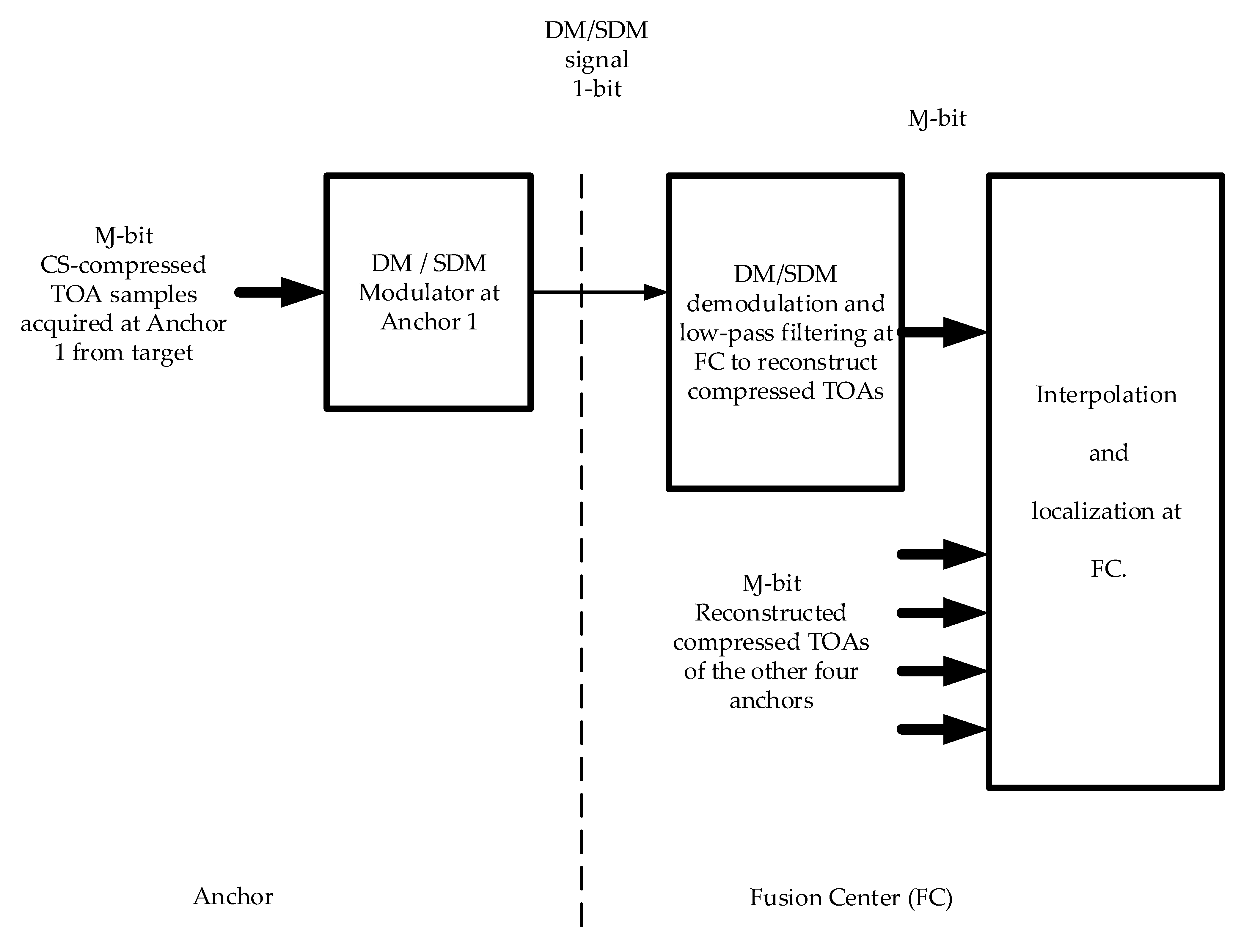
The present work attempts both CS and SWL directions simultaneously to reduce the communication energy expenditure by first applying CS to the data to be transmitted so as to reduce the number of samples and then applying DM or SDM to achieve a 1-bit representation per sample. We demonstrate the performance of this approach in the context of target tracking in WSNs as depicted in the block diagram of Figure 1. The CS-compressed TOA data are DM/SDM-modulated at the anchors before transmission to the fusion center where they are DM/SDM-demodulated, LP-filtered and interpolated to restore the original uncompressed TOA values. Then, localization or target tracking is achieved at the fusion center.
To the best of our knowledge, combining CS with SWL techniques has not been attempted in the literature. There are, however, several works on 1-bit CS [8,9,10] that are quite different from the present approach. In 1-bit CS, the limiting case of 1-bit measurements is considered by preserving just the sign information of random samples or measurements and treating the measurements as sign constraints to be enforced in reconstruction. The original signal is then recovered by constrained optimization to within a scaling factor since sign information does not include amplitude information. To resolve this ambiguity, reconstruction is constrained to be on the unit sphere to reduce the search space [8]. However, it has been shown in [11,12] that for target localization or tracking in WSNs, the computationally expensive recovery by convex optimization can be replaced by simple linear interpolation due to the usually low frequency content of TOA measurements from moving targets. In addition to its computational efficiency, linear interpolation can be made to operate in real time or with small delay whereas other optimization techniques such as -minimization are batch processing techniques requiring the whole or a considerably large part of the signal to be available to be processed for optimized reconstruction [4,13]. The proposed combined CS-SWL method suits the simple linear interpolation recovery scheme.
Referring to the system in Figure 1, some computation is still needed in the anchor nodes to implement a random number generator for CS random acquisition of the TOA samples, in addition to the simple hardware of the DM/SDM modulator. However, this is more than compensated for by the achieved communication energy efficiency. Localization at the fusion center is performed by the method of gradient descent (GD) [11,12,14].
The remainder of the paper is organized as follows. Section 2 discusses GD localization in WSNs based on CS. Section 3 overviews DM and SDM, whereas Section 4 explains their incorporation in the overall localization system and the ensuing parameter adjustments. Simulation results are presented in Section 5, and Section 6 concludes the paper.
2. CS-Based Gradient Descent Localization in WSNs
Localization in WSNs usually involves distance measurements between a target node and a number of reference nodes or anchors. Computing these distances by TOA data is most commonly adopted in low-density WSNs due to their insensitivity to inter-device distances compared to other types of data used in range-based localization such as time-difference-of-arrival (TDOA), received-signal-strength (RSS) or angle-of-arrival (AOA) data [15]. Iterative localization methods using GD are widely used due to their noise immunity compared to analytical methods [16] and low computational complexity [17].
We consider GD localization in three dimensions as in [11,12]. The error function to be minimized in this optimization problem is given by
with
where the target node needs N anchor nodes to be localized. For three dimensions, N is at least 4. The anchor nodes are with . The distance between the i-th anchor node and the target is , the receive time of the i-th anchor is , and the transmit time of the target is . Thus, is the TOA measurement acquired at the i-th anchor. Finally, c is the speed of light when RF or UWB signals are used in ranging.
GD minimization of the error function in Equation (1) is achieved by
where and are the vectors of position and gradient at the k-th iteration respectively, and α is the convergence factor. The iteration index k is also the time index when tracking is performed for a moving target.
The gradient vector at the k-th iteration is given by
CS can be used to acquire the TOA data for energy-efficient localization. Following is a brief overview of CS.
In compressive sensing, a discrete-time signal vector can be acquired or sampled compressively by a measurement or sampling matrix to yield the vector , , according to
Clearly, the above is an underdetermined system of equations in terms of the recovery of from . We assume that is K-sparse in the M-dimensional space spanned by the M basis vectors such that
where is the matrix whose columns consist of the M basis vectors, and s is the transform vector containing only K non-zero elements and K << M. In our case, is the DFT matrix. Therefore, Equation (5) becomes
CS theory states that the vector is recoverable from if the sparsity information of the former is preserved in the latter. This is possible if matrix satisfies the restricted isometry property (RIP) [18] which dictates the incoherence of with . This incoherence can be established by ensuring that is a random matrix which results in the vector being fully recoverable from when the following inequality is satisfied:
where C is a constant and by solving the convex optimization problem of the underdetermined system of equations using -minimization [4,19].
For localization in WSNs, CS can therefore be applied by random acquisition or sampling of the TOA data at the anchors at a rate below the Nyquist rate. It has been demonstrated in [11] that the TOA data associated with helical motion of the target node, for instance, is sufficiently sparse in frequency, thereby justifying the use of CS for energy-efficient tracking. Moreover, it has also been shown that the computationally complex and batch-processing -minimization can be replaced by simple linear interpolation of the compressed TOA data received at the fusion center as a computationally efficient and almost real-time recovery scheme of the original TOA data. This is possible because of the usually low-frequency content of TOA data, taking into account that interpolation is a low-pass filtering operation.
Thus far, a means to reduce communication energy consumption has been ensured by using CS to reduce the number of TOA samples transmitted from the anchors to the fusion center. A further reduction of this energy consumption component is to achieve a 1-bit representation per TOA sample by using DM before transmission. DM techniques are overviewed in the following section.
3. Overview of Delta Modulation Techniques
In the context of digital modulation techniques, delta modulators have a particularly simple architecture compared to pulse code modulation (PCM) systems. DM systems produce a bit stream that corresponds to their sampled inputs using oversampling to overcome quantization noise effects. In PCM, the output bit stream consists of blocks of Ɱ bits where each Ɱ-bit block represents the quantized sample amplitude of the PCM pulse [2]. Quantization is a non-invertible process because an infinite number of amplitudes are mapped to a finite number of quantization levels such that the original signal cannot be recovered exactly [3]. DM systems include the simple DM and the sigma delta modulator or SDM which overcomes some disadvantages of the former. In addition to their simple architecture, they enable the representation of Ɱ bits per sample by a single bit, thereby meeting the limited power consumption requirement in wireless sensor systems. DM and SDM are discussed next.
3.1. Delta Modulation
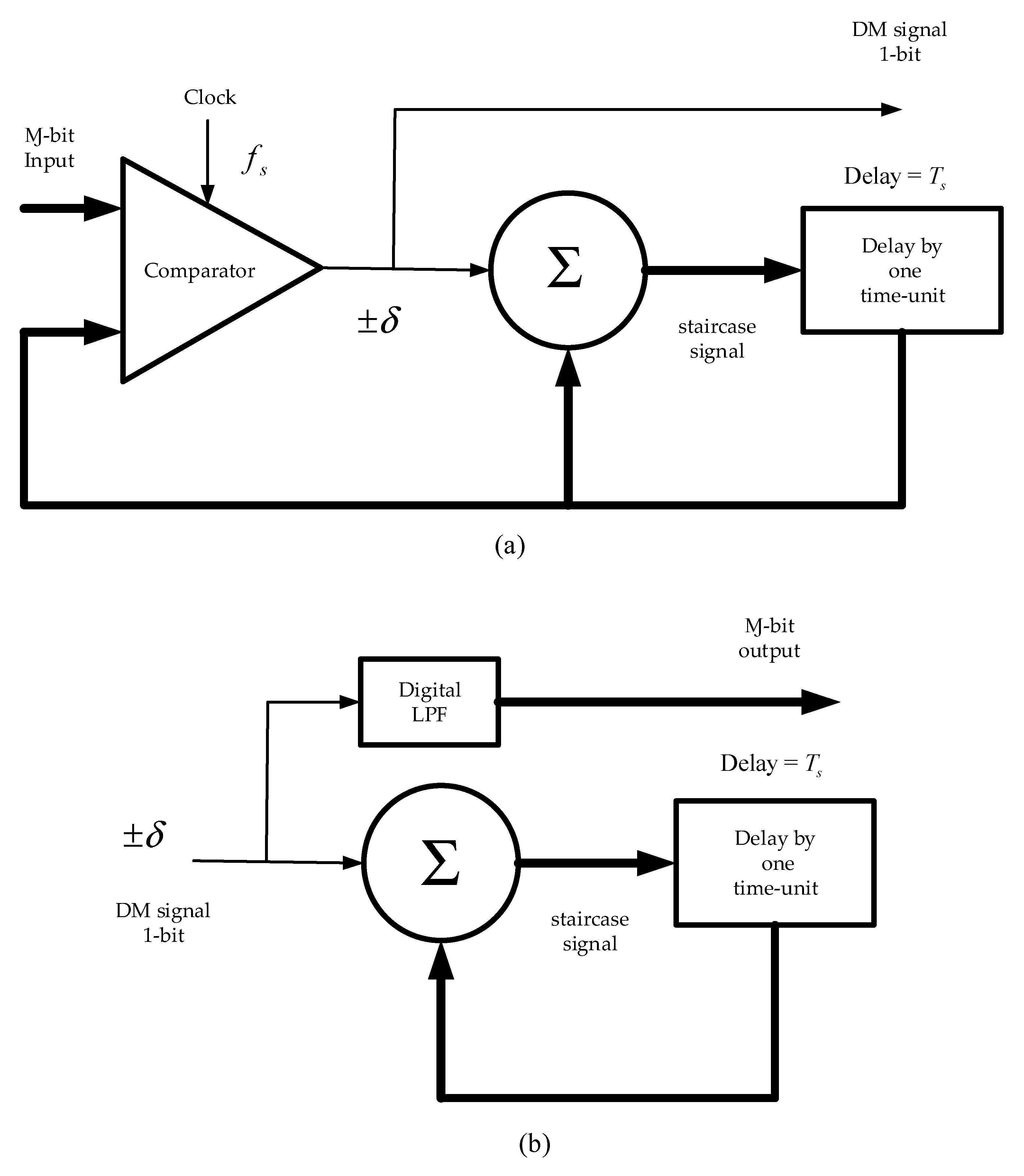
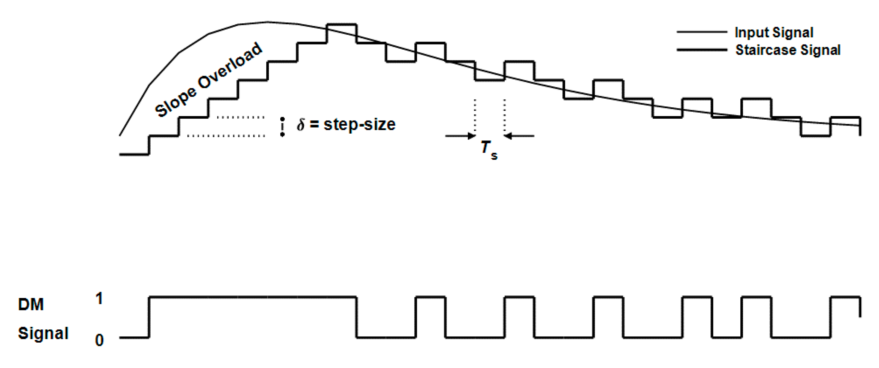
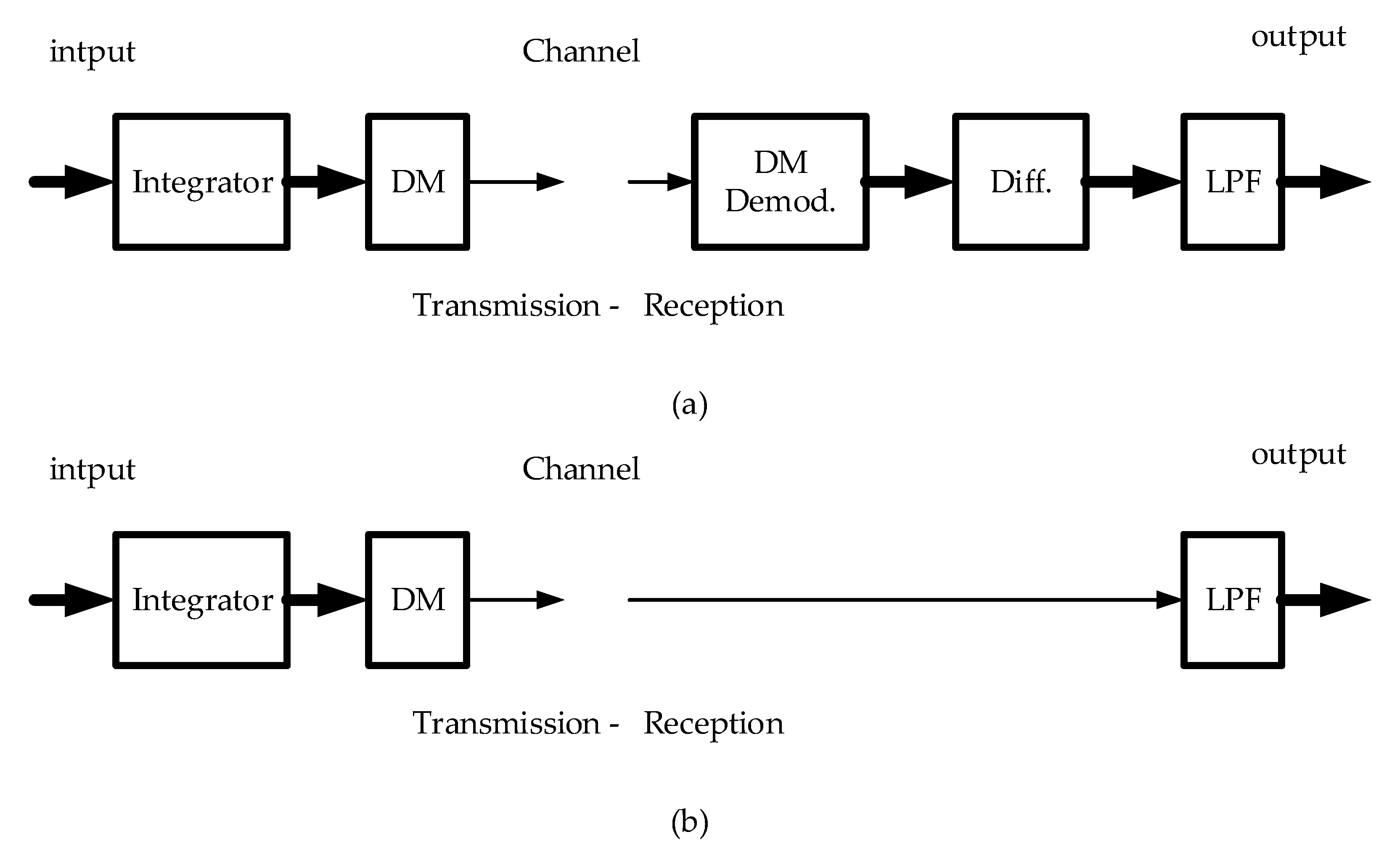
The DM scheme has initially been devised to reduce the complexity of PCM. Before describing DM, we wish to emphasize that while the DM analog-to-digital converter originally has an analog input, the input to the delta modulator used in the application under consideration in this work is a sampled discrete-time signal (the TOA samples). Without loss of generality, however, the DM operation remains essentially the same. The sequence of input samples is approximated by a sequence whose envelope is a staircase function moving above and below by one quantization level (δ) with each sample. Hence, a single binary digit corresponding to this up and down movement is sufficient to describe the DM operation for each sample. A ‘1’ is generated if the movement is upwards, for instance, and a ‘0’ otherwise, so that an output bit stream is produced. We call the output bit stream simply the DM signal. Figure 2 describes the DM transmission and reception systems, and Figure 3 illustrates an example of DM operation.
It is clear from the block diagram of Figure 2 that this is essentially a feedback process. For the transmission block diagram, it is clear that the input sample is compared to the previous approximating staircase function sample. A ‘1’ or ‘0’ is generated resulting in the addition of +δ or −δ, respectively, such that the staircase samples are always in the direction of the input samples. The binary bit stream is used in the receiver to reconstruct the staircase samples. The latter can then be smoothed by a low-pass filter to reduce quantization noise.
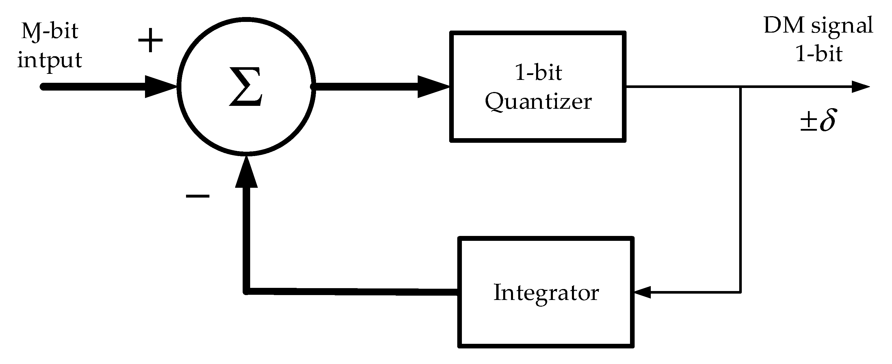
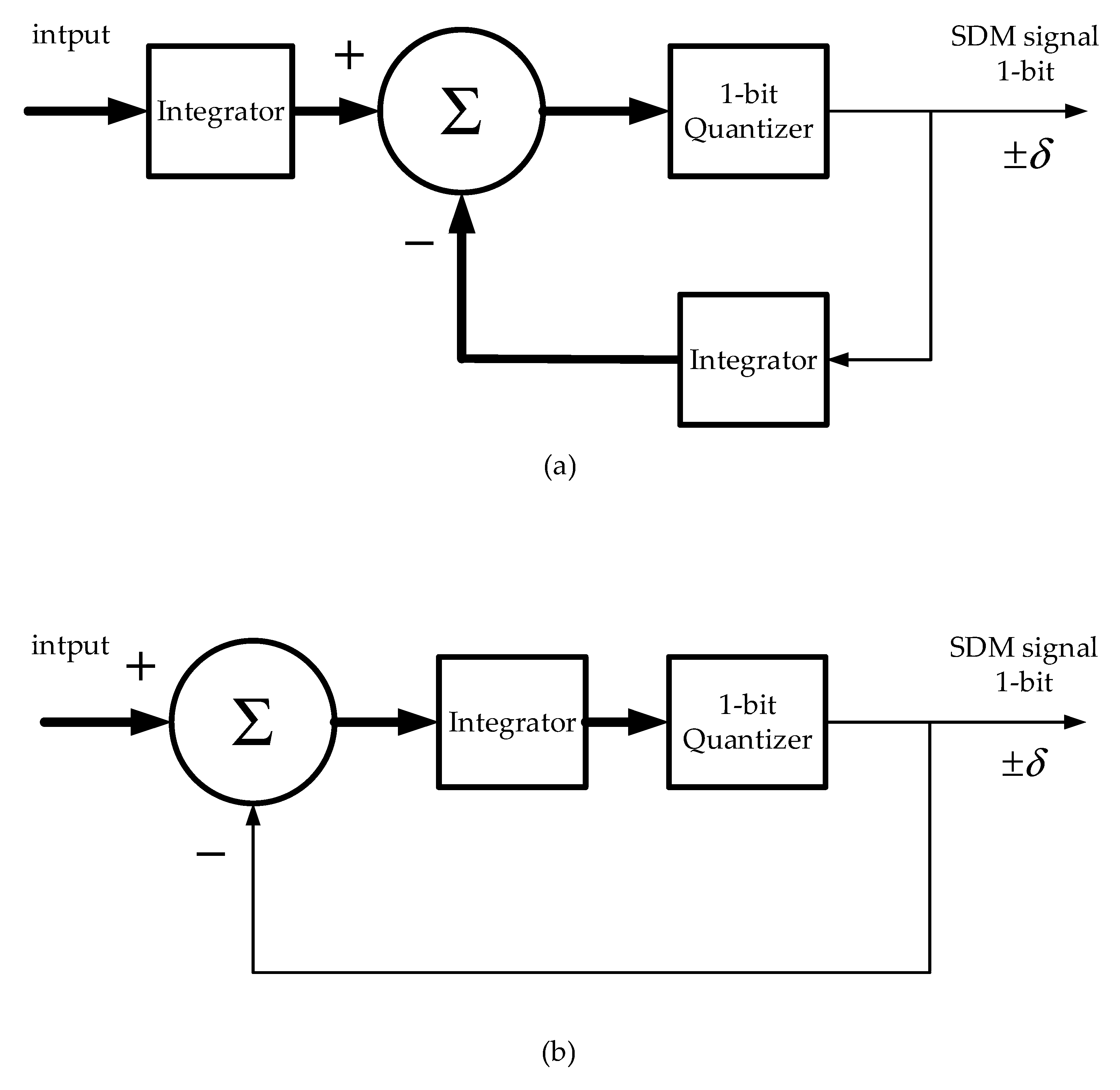
As shown in Figure 3, the step size δ must be chosen as a compromise between two types of errors that are to be avoided as much as possible. These are slope overload error and idling error. Slope overload occurs when the input samples are changing rapidly, and therefore, the staircase samples are unable to follow closely. This type of error increases with the decrease of δ and with the increase of high frequency content of the input samples. Idling error occurs when the input samples are changing very slowly, and it increases with the increase of δ. The accuracy of the DM scheme improves with the increase of the sampling rate [2]. The DM modulator of Figure 2a can also be depicted in block diagram form as in Figure 4.
Because slope overload increases with the increase in the frequency content of the input samples, simple DM becomes unsuitable when the input spectrum is flat. This can be overcome by using the SDM scheme described in the following subsection.
3.2. Sigma-Delta Modulation
The slope overload disadvantage of DM can be overcome by preceding the DM by an integrator in order to decrease the high frequency energy of the input samples [3,20]. This is depicted in Figure 5a. To retrieve the flat spectrum, a differentiator is then placed after the DM demodulator. A low-pass filter is also necessary to reduce quantization noise. However, since the demodulator is essentially an integrator, we can obtain the same effect at the receiver by omitting both demodulator and differentiator. The receiver will then consist only of the low-pass filter as shown in Figure 5b.
The name sigma-delta modulation comes from placing the integrator (sigma) before the delta modulator.
3.3. Oversampling, Noise Shaping and Low-Pass Filtering
Oversampling (OS) is a technique used in both DM and SDM systems to lower the noise floor of the input signal to the system. If the sampling frequency of the input is and the input is a single tone with noise, we know that the random noise extends from zero to of the input spectrum. If we now oversample by increasing the sampling frequency to , the SNR remains the same, but the noise energy will spread over a wider frequency range from zero to , causing the noise floor to drop and the SNR to increase after low-pass filtering at the receiver. The parameter is the oversampling ratio. Thus, OS by itself changes the distribution of the noise and not the total noise power. Although the most common application of SDM is analog-to-digital conversion (ADC), the use of SDM in the present work is confined to its ability to allow one-bit transmission per TOA sample for energy-efficient CS-based localization in WSNs. Hence, we dispense with some features of the traditional SDM such as the OS technique described above since OS contradicts the concept of CS and thereby cancels its benefits. OS is used to improve the resolution of classical ADC methods, which are not the objective of the present work. The assumption of OS dispensibility is true for many sensor applications where changes are slow such as those associated with bio-signals, temperature etc. [1].
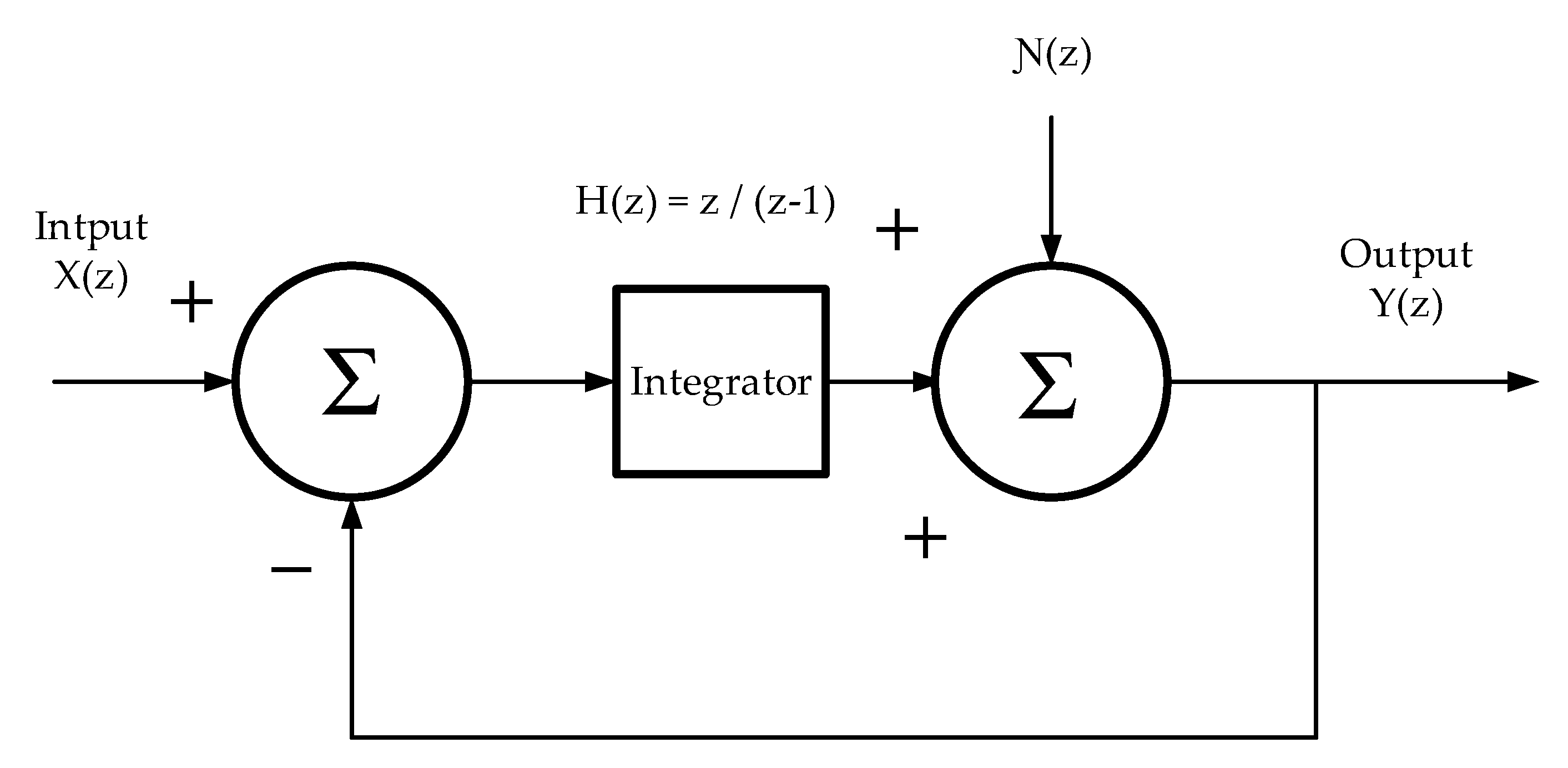
In SDM systems, the technique of noise shaping can remove more noise than can simple OS. To understand noise shaping, consider redrawing Figure 6b as in Figure 7 which is a z-domain representation and where the quantizer is replaced by a quantization noise source .
It is straightforward to show by superposition that
where and are the signal transfer function and the noise transfer function, respectively [1]. If is a simple integrator with transfer function given by , then it is easy to prove that SDM performs LP filtering on the signal and HP filtering on the noise. This is called noise shaping, the effect of which is to push the noise outside the band of interest where it is cancelled at the receiver by the LPF which averages the 1-bit SDM signal. The receiver LPF reconverts the signal back to a multi-bit one. The noise shaping property of SDM will be shown to have a significant effect on the performance of localization problem at hand, even when used without OS.
The following section describes the incorporation and analysis of the DM/SDM system in CS node localization for WSNs.
4. CS-DM/SDM Localization in WSNs
Both DM and SDM systems are considered for the application of WSN node localization and tracking employing CS in the anchor acquisition of the TOA samples sent from the target. Referring to Figure 1 of the introduction section, let us assume that the sample reduction ratio R regarding the CS operation is given by
Therefore, CS reduces the number of transmitted samples by R. If we further assume that each sample is represented by an Ɱ-bit word, then the total communication energy from anchor to fusion center, after applying CS and DM/SDM, is reduced by (R. Ɱ) owing to the 1-bit-per-sample representation enabled by DM/SDM.
The localization error criterion used to assess performance is chosen as the normalized error measure (NEM) given in dBs. This is a relative error measure involving the localization error function and the true distances of Equation (1), and is given by
where K is the iteration number, Ҡ is the total number of target path points, and N is the number of anchors.
Let us first consider the DM-based localization system. Under no-compression conditions (R = 1), operation can be almost free from quantization noise when the step size is optimized for best performance measured by NEM. Introducing CS to the system by randomly acquiring TOA values at the anchors and gradually increasing the maximum random sampling interval, we find that the succeeding DM system will exhibit slope overload because the input samples change abruptly in magnitude between successive randomly spaced samples. Thus, the effect of CS on the original uncompressed slowly varying TOA sequence is to introduce higher frequencies due to abrupt transitions caused by compression, thereby leading to slope overload. This necessitates re-optimizing (increasing) the DM step size every time the maximum sampling interval is increased until normal operation is resumed with no slope overload. The increasing step size will increase the quantization noise and hence decrease the localization accuracy at the fusion center. This is the major disadvantage of the DM system when used in conjunction with CS.
Noting the noise shaping property of the SDM system, its use instead of the DM system is expected to improve the overall performance or localization accuracy measured by NEM. However, the reconstruction LPF at the fusion center must be carefully designed. Moreover, the phase introduced by this filter introduces additional localization error. In contrast, the reconstruction filter used with CS-DM localization can be simple and does not introduce significant distortion; the reason is that the reconstruction filter filters the staircase waveform which is mainly of low frequency content, whereas in SDM, it filters the SDM signal itself which has a wider-range spectral content. Therefore, the filter to be used in this work in conjunction with CS-SDM will be chosen as a linear-phase optimal finite impulse response (FIR) digital filter employing the Parks–McClellan filter design algorithm [21]. The equiripple method of designing this type of filter is an optimization problem that adjusts the coefficient values to create an optimal filter such that the transition width is minimized along with the stopband and passband ripple.
In this work, we consider tracking a target moving along a helical path in three dimensions representing the moving-target position. These dimensions are described by the following equations:
We assume that the angle takes on the values from zero to 2π, and r and are constants. All anchors are assumed to be in the radio range of the target path. In [11,12], a helical path with r = 40 and = 20 was considered. It was shown that the TOA values as a function of time had low frequency content. Therefore, we consider 315 points in the path are enough to yield acceptable localization error.
To achieve CS, the complete vector of 315 discrete TOA samples is input to a random sampling algorithm to yield a shorter vector of TOA measurements as in Equation (5), only to be reconstructed later by interpolation at the fusion center. In Equation (5), the sampling matrix Φ has at most one non-zero value (unity) in each row. The random sampling that generates the compressed vector is based on the selection of samples separated by random periods. The random variable representing these random periods is uniformly distributed over the time interval []. Thus, the sampling instants indexed by the integer , are given by
where is the initial time instant, is the original sampling period and , is the discrete uniform distribution over the integer interval .
It is assumed that the fusion center knows the distribution generating the random sampling instants in order to maintain the structure of the original TOA samples. The interpolated or reconstructed TOA values are then used to localize the target path by gradient descent.
In the following section on simulation results, both localization systems employing CS-DM and CS-SDM will be simulated, discussed and compared.
5. Simulation Results
The moving target localization and tracking problem is simulated in MATLAB. The WSN considered is three-dimensional with a volume of cubic meters. Five anchors are selected such that they all are in the radio range of the target as it moves along a helical path according to Equation (12). The x-, y-, and z-dimensions of the anchors are taken as [10,100,10,100,90], [100,90,70,80,90] and [10,10,100,100,150] meters, respectively. The helix constants are , = 20 and varies from zero to 2π. The initial dimensions of the moving target location are taken as the point (50, 0, 0). The TOA data acquired at the anchors are assumed to be line-of-sight (LOS) arrivals only. In accordance with Figure 1, the TOA values from the target moving along its path are compressed at the anchors by random CS after sampling to 315 helical path points. In [11], the spectrum of the TOA data in a similar localization problem is shown to be sparse as required by CS, and its magnitude never reaches zero; therefore, sampling is inevitably sub-Nyquist. The random sampling period obeys a uniform distribution as discussed in Section 4, with = 1 and = 1 to 6. The localization error criterion is taken as NEM. The results for the CS-DM and CS-SDM localization systems will be presented separately first and then compared.
5.1. CS-DM System
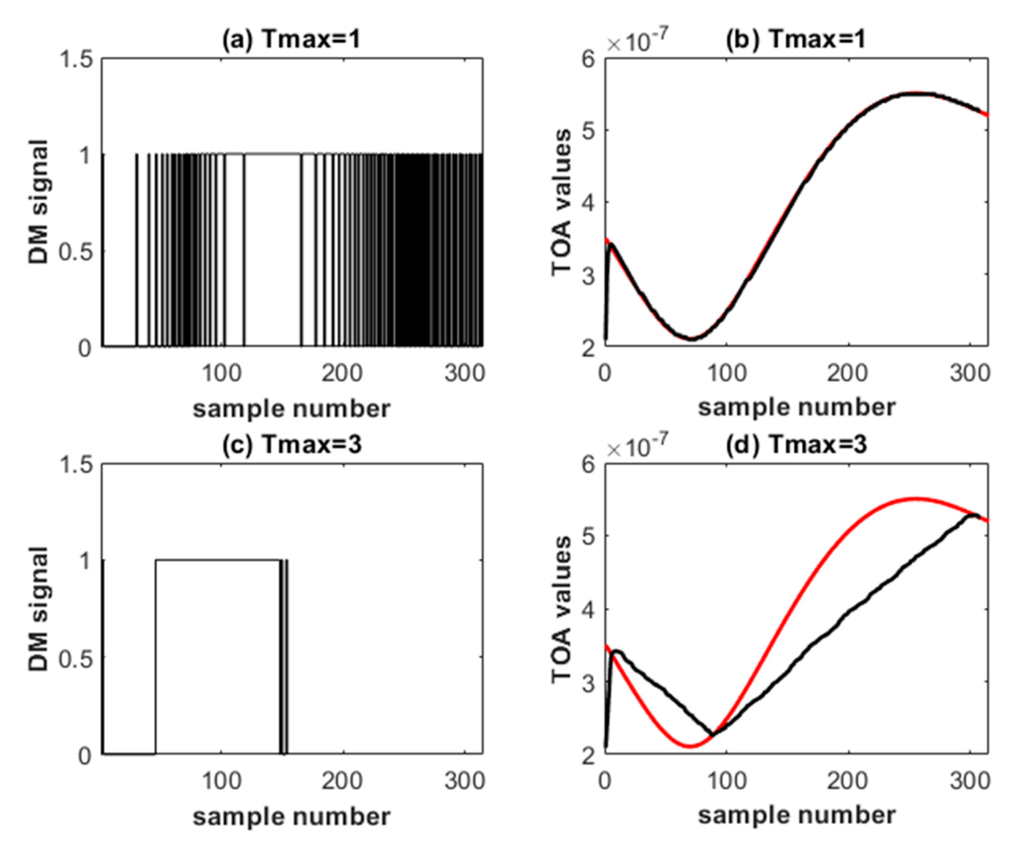
The system in Figure 1 is first simulated without CS ( = 1). The optimum DM step size δ was found to be 2.8 ns. The demodulation LPF of Figure 2b is a simple first order LPF to reduce the quantization noise. Localization is achieved at the fusion center with the GD algorithm using a convergence factor α = 0.24. This value has been optimized to yield the minimum NEM value of −39.54 dB. When calculating NEM, we discard the first erroneous 20 samples to take only the steady state localized points into account. Then, CS is incorporated with = 3, and the optimized δ in this case is 7 ns, resulting in NEM equal to −38.22 dB. As is increased, slope overload occurs, so it becomes necessary to increase the DM step size, and therefore, the quantization noise increases resulting in greater localization error even after step size optimization.
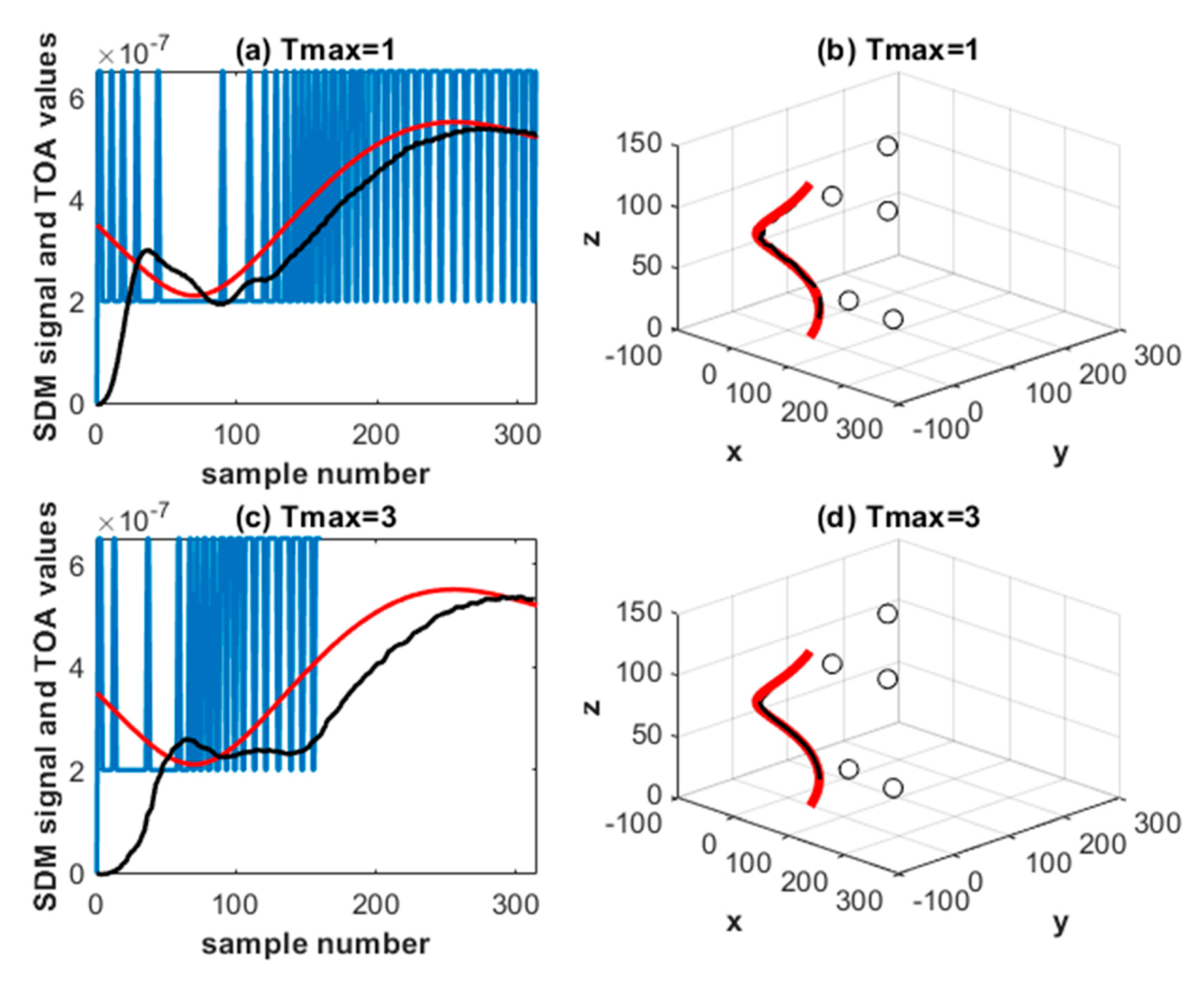
Figure 8 shows the DM signal and the original and reconstructed TOA values for both cases of = 1 and 3. With = 3, the average sampling interval is 2; that is why the corresponding DM signal in Figure 8c has half the number of original points. It is clear from Figure 8d that slope overload has occurred since the plot is for the original step size (2.8 ns) before optimization to the value of 7 ns. The increased localization error brought about by DM is compensated for by the achieved communication energy efficiency.
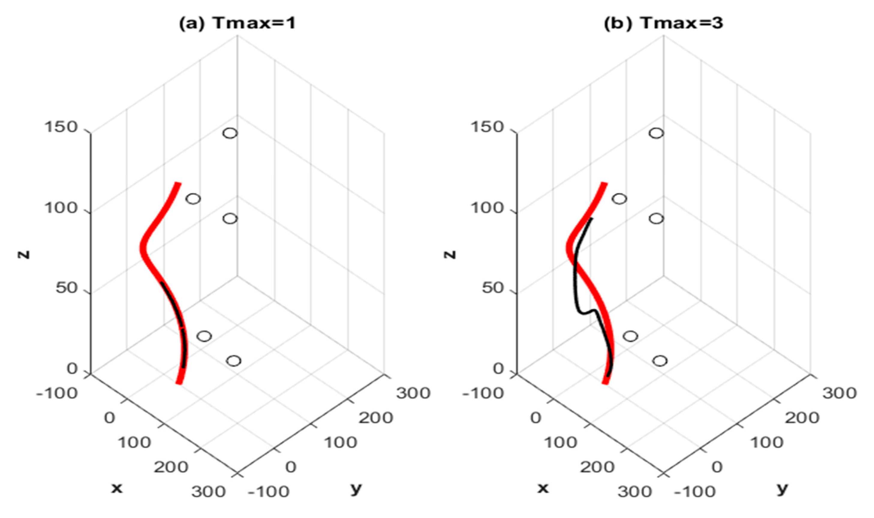
Figure 9 shows the true and localized 315-point path for the two cases of = 1 and 3. Both plots in Figure 9 are for the original step size of 2.8 ns. In Figure 9a ( = 1), the true and localized paths almost coincide. In Figure 9b ( = 3), the effect of slope overlaod on the localized path is clear. If the step size were optimized for = 3, then the corresponding path would be closer to that of = 1 (without CS). That is, the localization error would decrease, but it remains greater than that of the original settings without CS.
5.2. CS-SDM System
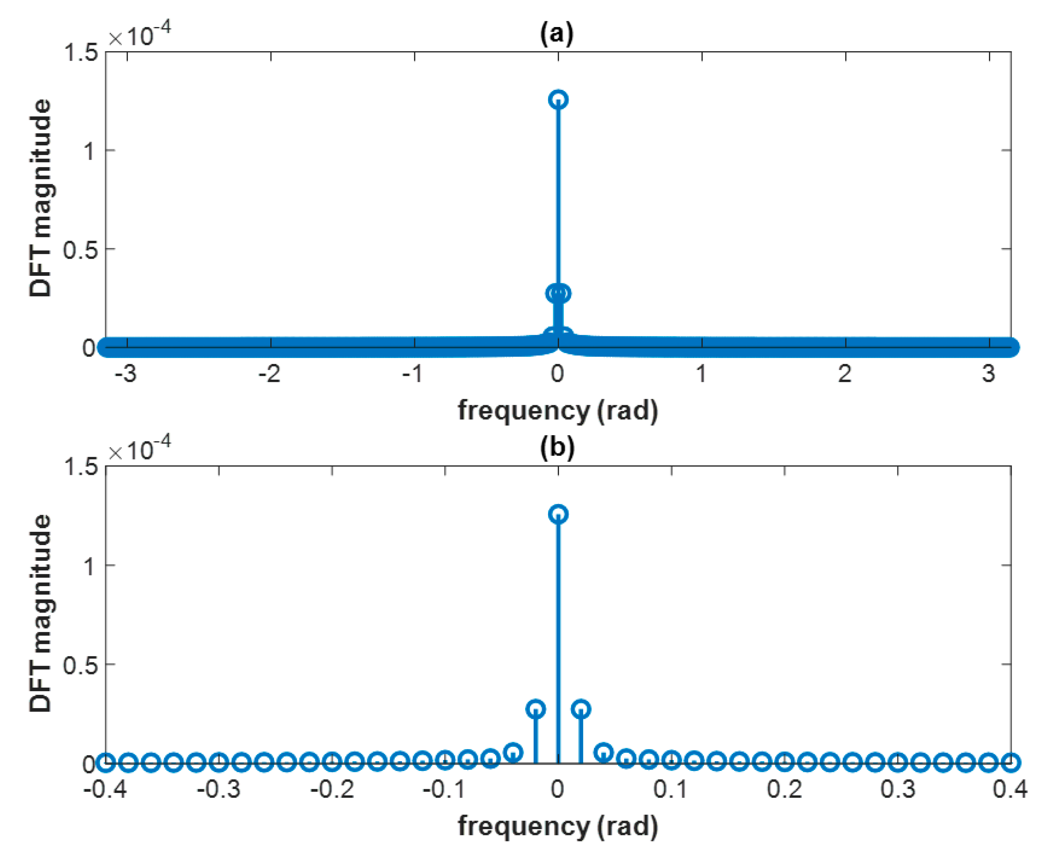
As in the previous subsection, the system in Figure 1 is simulated but using the SDM modulator of Figure 6b, resulting in the CS-SDM system. The convergence factor is the same for the CS-DM system for subsequent comparison. The LPF in the demodulator filters the SDM signal directly and therefore must be carefully designed to faithfully yield the reconstructed TOA values. The quantizer in Figure 6b is assigned the two levels 200 ns and 650 ns at its SDM output. These levels are first roughly chosen such that they are related to the exact TOA values so that when the SDM signal is filtered by the LPF, the reconstructed TOA values can be adjusted for minimum NEM by fine-tuning the two quantizer levels. For this purpose, the exact TOA values are obtained by setting in Equation (1) to zero and substituting the helical path positions, the anchor positions, and the speed of light. The DFT magnitude of the exact TOA waveform seen by Anchor 1 is shown in Figure 10. The position coordinates of Anchor 1 are (10, 100, 10). The system is first simulated with = 1 (no CS). The Parks–McClellan LPF filter discussed in Section 4 is designed according to the following specifications in Table 1 with a number of weights equal to 43.
It is clear from inspecting Figure 10 that the specified LPF passband of Table 1 includes the better part of the non-zero DFT values, and the stopband after the transition width is also well chosen.
The transfer function of this filter is shown in Figure 11. At DC frequency, the gain is slightly above 0 dB due to the equiripple property. It was found that multiplying the designed filter coefficients by 0.82 (that is multiplying the filter transfer function by a gain of 0.82) provides the best results; it gives a gain of almost 0 dB (unity) at DC frequency.
Under all the above conditions, and without CS, the resulting NEM is equal to −39.84 dB which is less than the corresponding DM case provided that the phase introduced by the LPF to the TOA values is subtracted. The phase causes a delay of 25 samples for this case of = 1. This is the major disadvantage of using CS-SDM although it yields significantly better results in terms of localization error if the phase delay is accounted for. For = 3, the value of NEM was found to amount to −39.7 dB after correcting a delay of 60 samples. Therefore, compared to the CS-DM system, CS in CS-SDM almost does not increase the localization error if the delay is corrected. Figure 12 demonstrates the CS-SDM localization system operation for the cases = 1 and 3. It is obvious from comparing Figure 12a,c that the phase introduced by the filter increases upon applying CS; the reason is that CS introduces higher frequencies to the TOA sequence and, therefore, to the SDM signal. This results in larger values of phase shift provided by the linear-phase FIR reconstruction filter used. However, the ensuing localization error can be eliminated if the delay is accounted for. This is evident from Figure 12b,d which are almost identical. This advantage of the CS-SDM system is due to the noise shaping property of SDM. Contrariwise, for the CS-DM system, the quantization error could not be removed totally even when step size is optimized.
5.3. Performance Comparison of CS-SWL Localization Systems
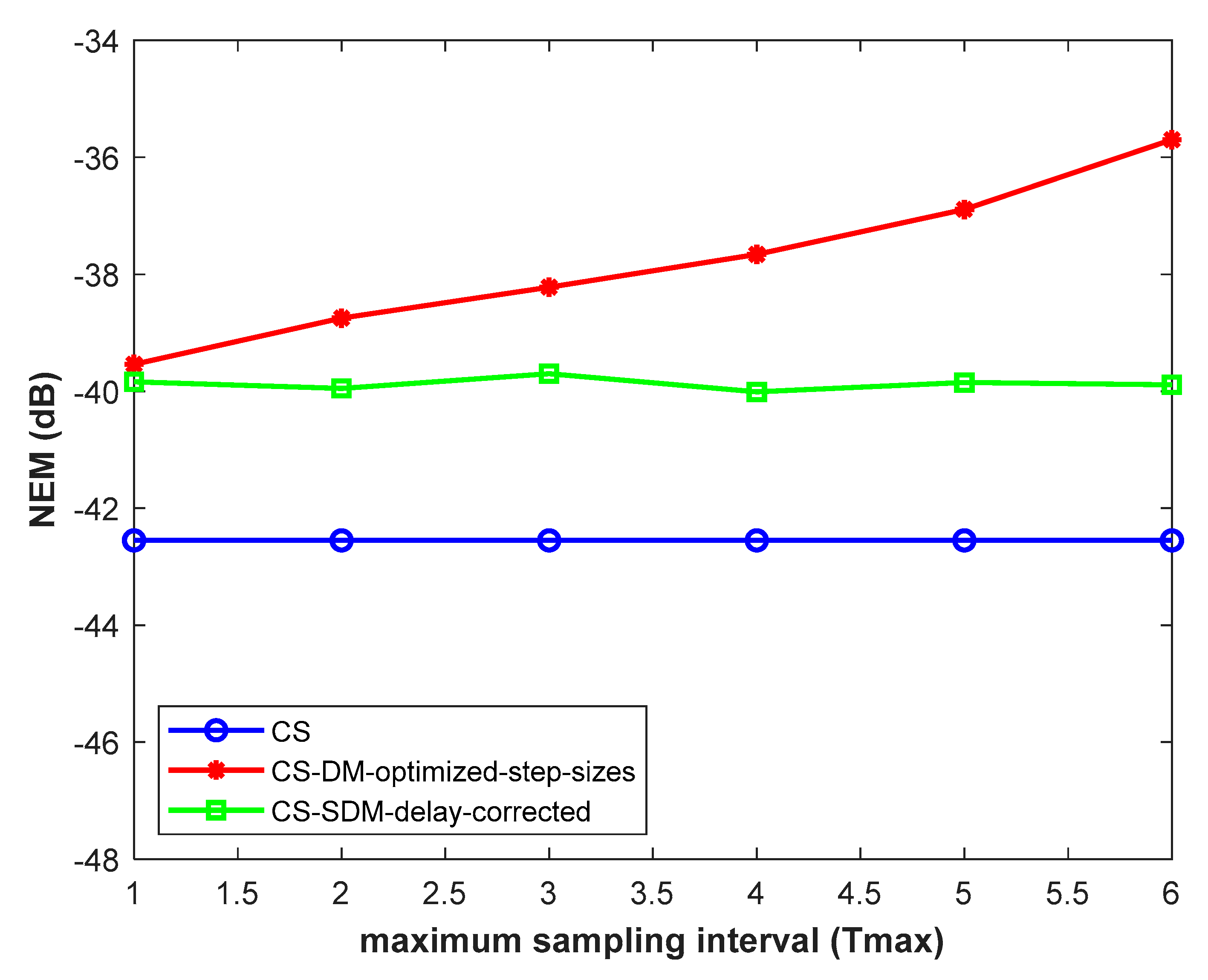
The performance in terms of NEM in dBs versus is shown in Figure 13 for the two considered CS-SWL systems together with the corresponding purely CS system. In this figure, the CS-DM system is optimized regarding its step size with the increase in . Likewise, the CS-SDM system is delay-corrected with every increase in the value of . The CS system exhibits a slightly better performance than the CS-SDM system in terms of localization error; however, the latter system is superior in terms of energy efficiency. The poorest performance is that of the CS-DM system on account of the necessary step size optimization process explained in Section 4, which increases the quantization noise and therefore the localization error although it would be better than the case in which no step size optimization is carried out as increases.
The extent to which can be increased is determined by the number of available samples of the TOA uncompressed sequence as the target moves along its path, as well as the permissible localization error achieved which is rather application-dependent. As discussed for the CS-DM system, increasing requires step size optimization (increase) which leads to increased quantization noise and hence increased localization error. As for the CS-SDM system, the increase in requires increased delay correction. This delay measured in number of samples must constitute a small amount compared to the total number of available TOA samples. For the problem under consideration in this work, the maximum value of = 6 was found suitable in terms of localization error as well as the path length of 315 points.
So far, we have assumed that the TOA values acquired at the anchors are free of measurement noise and that transmission from the anchors to the fusion center is noise-free. The considered transmission medium is taken as free space line of sight (LOS) which is the simplest wireless channel model without shadowing or multipath [22]. In practice, the TOA values calculated or measured at the anchors are subject to measurement noise which can be modeled as zero-mean additive white Gaussian noise (AWGN) with standard deviation that will be denoted by SD1. Moreover, the TOA discrete waveform (in case of pure CS) or the DM/SDM signals communicated between the anchors and fusion center are also subject to contamination by AWGN whose mean and standard deviation will be taken as zero and SD2, respectively. SD2 is found by specifying the SNR in dB’s and substituting it in
where P is the transmitted signal power between anchors and the fusion center. In the simulations, SD1 is assigned a value and incorporated in the measured TOA values by adding the corresponding noise component. As for SD2, it is computed from Equation (15) upon assigning an SNR value, and the corresponding noise component is added to the transmitted signal.
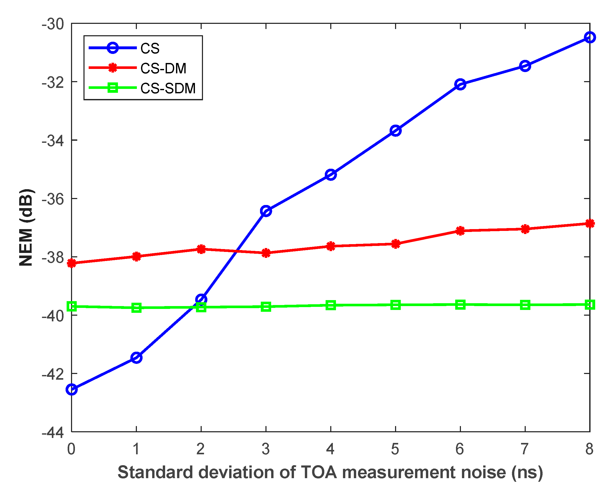
Figure 14 demonstrates NEM in dBs, for the three localization systems, versus SD1 in nanoseconds, where SD1 is the standard deviation of the TOA measurement noise, and for transmission SNR of 50 dB. is set to 3 in this figure, the DM step size for the CS-DM case is optimized at 7 ns, and the correction delay for the CS-SDM case is 60. The CS-DM system is the poorest for SD1, less than around 2.5 ns. However, for SD1 greater than 2.5 ns, the performance of CS-DM improves over the purely CS system because the quantization process will crop any measurement noise that causes the TOA sample to exceed the quantized value, provided that no slope overload occurs. This applies to the CS-SDM system as well which is, in addition, characterized by its noise shaping property, making it the recommended system for both energy efficiency and resilience to TOA measurement noise.
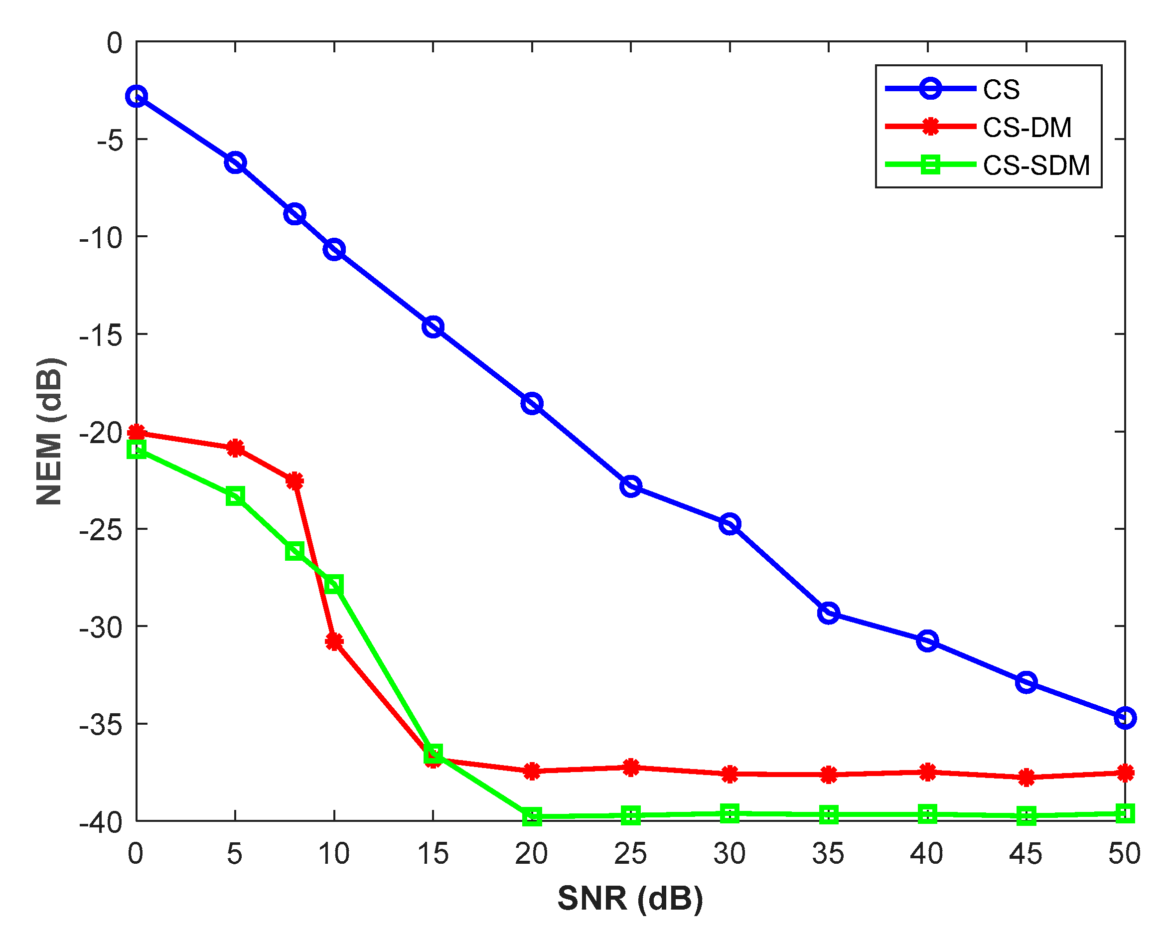
Figure 15 shows NEM in dBs versus SNR in dBs for the three localization systems while fixing SD1 to 5 ns. is set to 3, the DM step size for the CS-DM case is optimized at 7 ns, and the correction delay for the CS-SDM case is 60. It is clear that the pure CS system exhibits the lowest performance for the same reasons explained above for Figure 14 regarding the advantageous cropping of noise in the other two systems. The CS-SDM system is generally optimum.
Figure 16 shows the normalized communication energy consumption (E) for the three localization systems. This is measured by the total number of bits transmitted to localize the complete helical path of length 315 positions. The normalized energy consumption in transmitting one bit is taken as unity. Therefore, E for the CS system can be expressed as
and for the CS-DM and CS-SDM systems as:
In Figure 16, , for , and Ɱ is made variable as shown. The energy efficiency achieved using SWL is evident.
5.4. Final Remarks
Summarizing the results of Figure 13, Figure 14 and Figure 15, it is found that under noise-free conditions, the CS-DM/SDM localization systems have the sole advantage of communication energy efficiency only, but with higher localization error than the pure CS system. However, under measurement noise and transmission noise conditions, the CS-DM/SDM systems clearly outperform the CS system in terms of both energy efficiency and localization error particularly for measurement noise standard deviation SD1 greater than 2 ns and for all the range of possible transmission SNR values.
Whether under noise-free or noisy operating conditions, the significant communication energy efficiency achieved with the CS-DM/SDM systems and illustrated in Figure 16 indicates the importance of implementing them despite the additional hardware since energy considerations are of paramount importance in WSNs.
6. Conclusions
Three GD localization systems of a moving target within a WSN are simulated and compared with the aim of achieving the greatest possible communication energy efficiency without degrading performance. The three systems are pure CS localization, CS-DM and CS-SDM localization systems which employ, in addition to CS, short word-length techniques leading to energy efficiency. Under noise-free conditions, the optimum system in terms of both energy efficiency and localization error is found to be the CS-SDM localization system due to the noise shaping property of SDM. The poorest performance in terms of localization error is the CS-DM system; still, it is a possible choice due to the achieved energy efficiency. Both CS-DM/SDM schemes, especially the system involving SDM, proved resilient to TOA measurement noise, as compared to the pure CS localization system, and gave better performance than the latter in terms of both localization error and energy efficiency due to the noise cropping advantage of quantization, the noise shaping property particular to SDM and the decrease of the number of transmitted bits to the fusion center. The CS-DM/SDM schemes also outperformed the CS system in the presence of AWGN in the transmission path from the anchors to the fusion center. This advantage is particularly evident for low SNRs. The small additional hardware complexity caused by CS-DM/SDM, as compared to pure CS, is counteracted by the improved performance under AWGN and by the significant communication energy efficiency achieved.
Author Contributions
Conceptualization, Z.M.H. and N.A.S.A.; methodology, N.A.S.A. and Z.M.H.; software, N.A.S.A. and Z.M.H.; formal analysis, N.A.S.A. and Z.M.H.; investigation, N.A.S.A. and Z.M.H.; resources, N.A.S.A. and Z.M.H.; writing—original draft preparation, N.A.S.A.; writing—review and editing, Z.M.H. and N.A.S.A.; supervision, Z.M.H. All authors have read and agreed to the published version of the manuscript.
Funding
This research is partially funded by Edith Cowan University via the ASPIRE Program.
Data Availability Statement
The MATLAB code for this work is available from the authors on request.
Acknowledgments
The authors would like to thank Edith Cowan University for supporting this project via the ASPIRE Program. Thanks and appreciation are also due to the anonymous reviewers for their constructive comments and to the MDPI office for prompt response and valuable guidance throughout the review process.
Conflicts of Interest
The authors declare no conflict of interest.
References
- Hussain, Z.M. Energy-Efficient Systems for Smart Sensor Communications. In Proceedings of the 2020 30th International Telecommunication Networks and Applications Conference (ITNAC), IEEE, Melbourne, Australia, 25–27 November 2020; pp. 1–4. [Google Scholar]
- Stallings, W. Data and Computer Communications, 9th ed.; Pearson: Upper Saddle River, NJ, USA, 2011. [Google Scholar]
- Aziz, P.M.; Sorensen, H.V.; Van der Spiegel, J. An overview of sigma-delta converters. IEEE Signal Process. Mag. 1996, 13, 61–84. [Google Scholar] [CrossRef]
- Candes, E.J.; Wakin, M.B. An introduction to compressive sampling. IEEE Signal Process. Mag. 2008, 25, 21–30. [Google Scholar] [CrossRef]
- Qaisar, S.; Bilal, R.M.; Iqbal, W.; Naureen, M.; Lee, S. Compressive sensing; from theory to applications, a survey. J. Commun. Netw. 2013, 15, 443–456. [Google Scholar] [CrossRef]
- Bilinskis, I.; Selavo, L.; Sudars, K. Method for sensor data alias-free acquisition from wideband signal sources and their asymmetric compression reconstruction. Balt. J. Mod. Comput. 2013, 1, 199–209. [Google Scholar]
- Tarczynski, A.; Allay, N. Spectral analysis of randomly sampled signals: Suppression of aliasing and sample jitter. IEEE Trans. Signal Process. 2004, 12, 3324–3334. [Google Scholar] [CrossRef]
- Boufounos, P.T.; Baraniuk, R.G. 1-Bit Compressive Sensing. In Proceedings of the 42nd Annual Conference on Information Sciences and Systems (CISS’08), Princeton, NJ, USA, 19–21 March 2008; IEEE: Princeton, NJ, USA; pp. 16–21. [Google Scholar]
- Yin, M.; Yu, K.; Wang, Z. Compressive sensing based sampling and reconstruction for wireless sensor array network. Math. Probl. Eng. 2016, 2016, 11. [Google Scholar] [CrossRef] [Green Version]
- Shen, L.; Suter, B.W. One-Bit compressive sensing via lo-minimization. EURASIP J. Adv. Signal Process. 2016. [Google Scholar] [CrossRef] [Green Version]
- Alwan, N.A.S.; Hussain, Z.M. Compressive sensing for localization in wireless sensor networks: An approach for energy and error control. IET Wirel. Sens. Syst. 2018, 8, 116–120. [Google Scholar] [CrossRef]
- Alwan, N.A.S.; Hussain, Z.M. Compressive sensing with chaotic sequences: An application to localization in wireless sensor networks. Wirel. Pers. Commun. 2019, 105, 941–950. [Google Scholar] [CrossRef]
- Chen, W.; Wassell, I.J. Energy-efficient signal acquisition in wireless sensor networks: A compressive sensing framework. IET Wirel. Sens. Syst. 2012, 2, 1–8. [Google Scholar] [CrossRef] [Green Version]
- Qiao, D.; Pang, G.K.H. Localization in Wireless Sensor Networks with Gradient Descent. In Proceedings of the IEEE Pacific Rim Conference on Communications, Computers and Signal Processing, Victoria, BC, Canada, 23–26 August 2011. [Google Scholar]
- Patwari, N.; Ash, J.N.; Kyperountas, S.; Hero, A.O., III; Moses, R.L.; Correal, N.S. Locating the nodes. IEEE Signal Process. Mag. 2005, 22, 54–69. [Google Scholar] [CrossRef]
- Zhang, L.; Tao, C.; Yang, G. Wireless positioning: Fundamentals, systems and state-of-the-art signal processing techniques. In Cellular Networks- Positioning, Performance Analysis, Reliability; InTech: Rijeka, Croatia, 2011. [Google Scholar]
- Alwan, N.A.S.; Hussain, Z.M. Gradient descent localization in wireless sensor networks. In Wireless Sensor Networks, Insights and Innovations; InTech: Rijeka, Croatia, 2017. [Google Scholar]
- Candes, E.J.; Romberg, J. Sparsity and incoherence in compressive sampling. Inverse Probl. 2007, 23, 969. [Google Scholar] [CrossRef] [Green Version]
- Candes, E.J.; Romberg, J.; Tao, T. Robust uncertainty principles; exact signal reconstruction from highly incomplete frequency information. IEEE Trans. Inf. Theory 2006, 52, 489–509. [Google Scholar] [CrossRef] [Green Version]
- Flood, J.E. Digital Modulation. In Telecommunications Engineer’s Reference Book; Elsevier Ltd.: Oxford, UK, 1993. [Google Scholar]
- Lyons, R.G. Understanding Digital Signal Processing, 3rd ed.; Prentice-Hall, Pearson Education, Inc.: Upper Saddle River, NJ, USA, 2011. [Google Scholar]
- Molisch, A.F. Wireless Communications, 2nd ed.; Wiley: Chichester, UK, 2011. [Google Scholar]
Figure 1.
Combined CS-SWL communication-energy-efficient localization wireless sensor system using five anchor or reference nodes. Note that thick arrows are used for multibit connections.
Figure 1.
Combined CS-SWL communication-energy-efficient localization wireless sensor system using five anchor or reference nodes. Note that thick arrows are used for multibit connections.

Figure 2.
Delta modulation: (a) Transmission (DM modulator as a comparator and integrator in a feedback loop); (b) Reception (DM demodulator as an integrator and LPF).
Figure 2.
Delta modulation: (a) Transmission (DM modulator as a comparator and integrator in a feedback loop); (b) Reception (DM demodulator as an integrator and LPF).

Figure 3.
Example of delta modulation operation.

Figure 4.
Block diagram of the DM modulator of Figure 2a.
Figure 4.
Block diagram of the DM modulator of Figure 2a.

Figure 5.
Sigma-delta modulation (SDM): (a) derivation of SDM; (b) SDM system.

Figure 6.
SDM modulator: (a) as a DM modulator preceded by an integrator; (b) equivalent SDM modulator block diagram.
Figure 6.
SDM modulator: (a) as a DM modulator preceded by an integrator; (b) equivalent SDM modulator block diagram.

Figure 7.
SDM modulator in the z-domain.

Figure 8.
DM signals with original and reconstructed TOA values for the CS-DM localization system. The original TOA values are shown in red, the reconstructed in black. Results are averaged over 100 realizations.
Figure 8.
DM signals with original and reconstructed TOA values for the CS-DM localization system. The original TOA values are shown in red, the reconstructed in black. Results are averaged over 100 realizations.

Figure 9.
True and localized helical paths for the cases = 1 and 3. The true path is shown in bold red. The small circles indicate the five anchor positions. Results are averaged over 100 realizations.
Figure 9.
True and localized helical paths for the cases = 1 and 3. The true path is shown in bold red. The small circles indicate the five anchor positions. Results are averaged over 100 realizations.

Figure 10.
(a) The DFT magnitude of the TOA sequence seen by Anchor 1. (b) A magnified view.

Figure 11.
Demodulation LPF transfer function for the CS-SDM localization system.

Figure 12.
SDM signals, original and reconstructed TOA values and localized paths for the CS-SDM localization system. The original TOA values are shown in red and the reconstructed in black. True and localized helical paths are also shown. The true path is shown in bold red. The small circles indicate the five anchor positions. Results are averaged over 100 realizations.

Figure 13.
Performance of CS-SWL localization systems in terms of localization NEM versus maximum sampling interval () under noise-free conditions (neither measurement nor transmission noise). Results are averaged over 100 realizations.
Figure 13.
Performance of CS-SWL localization systems in terms of localization NEM versus maximum sampling interval () under noise-free conditions (neither measurement nor transmission noise). Results are averaged over 100 realizations.

Figure 14.
Localization NEM versus standard deviation of TOA measurement noise (SD1) for the three localization systems. = 3. Results are averaged over 100 realizations.
Figure 14.
Localization NEM versus standard deviation of TOA measurement noise (SD1) for the three localization systems. = 3. Results are averaged over 100 realizations.

Figure 15.
Localization NEM versus SNR for the three localization systems. = 3, standard deviation of TOA measurement noise SD1 = 5 ns. Results are averaged over 15 realizations.
Figure 15.
Localization NEM versus SNR for the three localization systems. = 3, standard deviation of TOA measurement noise SD1 = 5 ns. Results are averaged over 15 realizations.

Figure 16.
Normalized communication energy consumption for the three localization systems versus the number of bits/word (Ɱ) of the original TOA samples. R = 3, N = 5, path length = 315.
Figure 16.
Normalized communication energy consumption for the three localization systems versus the number of bits/word (Ɱ) of the original TOA samples. R = 3, N = 5, path length = 315.


Table 1.
SDM reconstruction LPF specifications.
| Band (rad) | Gain | Ripple |
|---|---|---|
| Passband: (0–0.04π) or (0–0.126 rad) | 1 | 5 dB |
| Stopband: (0.1π–π) or (0.314–3.14 rad) | 0 | −40 dB |
Publisher’s Note: MDPI stays neutral with regard to jurisdictional claims in published maps and institutional affiliations. |
© 2021 by the authors. Licensee MDPI, Basel, Switzerland. This article is an open access article distributed under the terms and conditions of the Creative Commons Attribution (CC BY) license (https://creativecommons.org/licenses/by/4.0/).
Share and Cite
MDPI and ACS Style
Alwan, N.A.S.; Hussain, Z.M. Short Word-Length Entering Compressive Sensing Domain: Improved Energy Efficiency in Wireless Sensor Networks. Information 2021, 12, 415. https://0-doi-org.brum.beds.ac.uk/10.3390/info12100415
AMA Style
Alwan NAS, Hussain ZM. Short Word-Length Entering Compressive Sensing Domain: Improved Energy Efficiency in Wireless Sensor Networks. Information. 2021; 12(10):415. https://0-doi-org.brum.beds.ac.uk/10.3390/info12100415
Chicago/Turabian StyleAlwan, Nuha A. S., and Zahir M. Hussain. 2021. "Short Word-Length Entering Compressive Sensing Domain: Improved Energy Efficiency in Wireless Sensor Networks" Information 12, no. 10: 415. https://0-doi-org.brum.beds.ac.uk/10.3390/info12100415
Note that from the first issue of 2016, this journal uses article numbers instead of page numbers. See further details here.