
A Personalized Compression Method for Steady-State Visual Evoked Potential EEG Signals


1
Institute of Semiconductors, Chinese Academy of Sciences, Beijing 100083, China
2
University of Chinese Academy of Sciences, Beijing 100049, China
*
Author to whom correspondence should be addressed.
Information 2022, 13(4), 186; https://0-doi-org.brum.beds.ac.uk/10.3390/info13040186
Submission received: 16 March 2022
/
Revised: 31 March 2022
/
Accepted: 5 April 2022
/
Published: 6 April 2022
(This article belongs to the Special Issue Biomedical Signal Processing and Data Analytics in Healthcare Systems)
Abstract
:As an informative electroencephalogram (EEG) signal, steady-state visual evoked potential (SSVEP) stands out from many paradigms for application in wireless wearable devices. However, its data are usually enormous, occupy too many bandwidth sources and require immense power when transmitted in the raw data form, so it is necessary to compress the signal. This paper proposes a personalized EEG compression and reconstruction algorithm for the SSVEP application. In the algorithm, to realize personalization, a primary artificial neural network (ANN) model is first pre-trained with the open benchmark database towards BCI application (BETA). Then, an adaptive ANN model is generated with incremental learning for each subject to compress their individual data. Additionally, a personalized, non-uniform quantization method is proposed to reduce the errors caused by compression. The recognition accuracy only decreases by 3.79% when the compression rate is 12.7 times, and is tested on BETA. The proposed algorithm can reduce signal loss by from 50.43% to 81.08% in the accuracy test compared to the case without ANN and uniform quantization.
1. Introduction
Brain data from hospitals, research laboratories, and consumer neuroscience devices can be used to understand the structure and function of the brain to improve individual health [1]. The brain–computer interface (BCI) is moving from laboratory to practical applications, and from wired transmission to wireless transmission. However, the amount of electroencephalogram (EEG) signal data needed is huge, which causes some difficulties for wireless transmission and forms a bottleneck to the practicability of the brain–computer interface. For example, there is currently more than 130TB of neural data for research on the image and data archive (IDA), which is a neurocognitive data-sharing platform. The EEG signal is promising in neuroscience applications, among the various other signals used in the brain–computer interface.
In addition, BCI technology is developing in the wireless direction because it has the significant advantage that its users can use it conveniently for a long time. During the test, the user’s activity range is not limited, and the neural activities can be monitored all day, which provides a greater possibility for in-depth research by medical experts and neuroscientists [2,3].
However, the more data these wireless devices collect, the more data are transmitted from the sensor end to the decoder end of the wireless system, which requires a higher bandwidth for the transmission and a large amount of wireless bandwidth resources, computing power, and transmission power. These restrictions hinder the implementation of a wearable brain–computer interface [4].
One of the most suitable application scenarios for EEG compression is the steady-state visual evoked potential (SSVEP) experiment [5,6,7,8,9,10]. The BCI speller based on SSVEP has many advantages in that it does not require user training, and its detection algorithm can be trained without relying on a large amount of training data. It has an excellent signal-to-noise ratio, high information transmission rate, and multi-classification ability [11,12]. To the best of our knowledge, there is a large amount of research on the detection algorithm of SSVEP [12,13,14], but little research on its compression.
SSVEP is a common application form of EEG signals. As shown in Figure 1a–c, when a specific frequency of visual stimulation is presented to the eyes, the brain will reflect neural signals consistently with the visual stimulation frequency or its harmonic frequencies in EEG, resulting in an SSVEP signal [15]. In the wireless context, after the user receives visual stimulation in the monitor, the EEG signal is captured by the collector, wirelessly transmitted to the data-processing device, and then fed back to the monitor by the device. Due to the specific frequency stimulation, the SSVEP signal has strong energy concentrated at some individual frequency points, as shown in Figure 1d. The signal characteristics of SSVEP have different specificities according to different subjects, and the signal quality varies greatly from person to person.
According to this characteristic, this paper proposes a personalized compression framework for SSVEP. To ensure that the individual SSVEP signal is compressed in the most effective manner, we propose a method combining incremental learning ANN [16,17,18] and non-uniform quantization to adapt to the different characteristics of different human SSVEP signals to ensure that its detection performance does not significantly degrade. First, the signal was DCT transformed and the main components were selected, and then incremental learning was used to generate an adaptive ANN model for each subject. After decompression with ANN, the difference between the recovered and original values was calculated to correct the error, and then personalized non-uniform quantization was used to reduce the error. Finally, inverse discrete cosine transformation (IDCT) was carried out to obtain the recovered signal close to the input signal. The compression result of the ANN model and the quantized error value were transmitted as compressed data. When the compression ratio was 12.7 times, the recognition accuracy decreased by only 3.79%. Compared with the case without ANN and uniform quantization, adaptive ANN improved the signal quality by from 9.91% to 15.67%, and non-uniform quantization improved this by from 46.32% to 90.98%. Under the condition of ensuring the test accuracy, the method showed an overall improvement of from 50.43% to 81.08%. Therefore, these methods are helpful to promote the practicability of wearable brain–computer interface devices based on SSVEP.
The rest of this paper is arranged as follows: Section 2 introduces the database, algorithm, adaptive ANN training method, and non-uniform quantization calculation method; Section 3 shows the effect of the two methods on the compression results; Section 4 discusses the impact of compressed data on SSVEP detection; Section 5 draws a conclusion.
2. Materials and Methods
2.1. Dataset
Since this scheme requires a directional design for SSVEP, the relevant data set of SSVEP was selected in the experiment. The benchmark database towards BCI application (BETA) is a large benchmark database for SSVEP-BCI applications [19]. The dataset contained the 64-channel EEG signals of 70 subjects, its task was a 40-target cued-spelling task, and each subject had four blocks of experiments. The 40 targets were arranged as a QWERTY virtual keyboard to conform to usage habits. The stimulation frequency range of the 40 targets was from 8 to 15.8 Hz, with a frequency interval Hz and a phase interval of . The original sampling rate of the signal was 1000 Hz, the passband range of the hardware filter was 0.15–200 Hz, and a notch filter was used to remove the 50 Hz frequency interference of the power supply. In the software processing stage, a band-pass filter was used to remove environmental noise. The signal was then down-sampled to 250 Hz. Each subject received an experimental stimulation from each target for 2 or 3 s.
2.2. Overall Structure
The proposed compression system was divided into two parts: the compressor and decompressor. The system structure is shown in Figure 2.
The compressor contains three steps: DCT transformation, neural network feature extraction, and quantization of differences. In the SSVEP task, the EEG signals were stimulated by a specific frequency and showed the corresponding frequency characteristics. Hence, the characteristics of these signals in the frequency domain were easier to extract than those in the time domain. DCT transform can extract the frequency components of each signal because, for the raw data, most signal energy is concentrated in some limited low-frequency components [20]. DCT transform, as the first step, was combined with an ANN-based compression scheme. Specifically, as shown in Figure 2, the DCT transform was applied to the input signal in the first step, and then some low-frequency coefficients were selected, which are called the main coefficients.
The calculation formula of DCT transform is:
where
Then, the DCT coefficients obtained by the transformation were selected. Since the DCT signal reflects the strength of the original signal at different frequencies, we can square the single point to obtain the spectral energy corresponding to each coefficient point, calculating the energy spectrum of each signal and averaging all the signals in the dataset to obtain the energy distribution of the SSVEP signal in the DCT transformed domain [21]. As shown in Figure 3, the energy of the first 80 coefficients accounted for a significantly larger proportion of the total 250 points than the rest of the coefficients, so the first 80 points were selected as the main components.
Compress the main components with a neural network to obtain the compressed coefficient , and then restore it with a neural network (see Section 2.3 for details) to obtain :
Then, create zero-padding on , and make this up to points to reconstruct the DCT coefficient:
Compare the reconstructed DCT coefficients with the original coefficients to obtain the error :
In order to compress the error, we were required to build a quantization table. Traditional methods mostly use uniform quantization, but this paper proposes the concept of non-uniform quantization for SSVEP. According to the statistical characteristics of different positions, the method uses different quantization tables to quantize the corresponding coefficients (see Section 2.4 for details).
and are the compressed signal. After transmission, the two sets of numbers arrived at the decompressor and were then decompressed by the decompressor. underwent a similar procedure as in the compressor, yielding . was subjected to the inverse quantizer to obtain the estimated value of .
From this, reconstructed DCT coefficients were obtained by adding the estimated DCT coefficients and the estimated error . The difference between and the original DCT coefficients was smaller than that of the direct estimation . Then, inverse DCT transform was performed on the coefficient to obtain the reconstructed value of the original EEG signal, as shown in Equations (10) and (11).
In this way, a relatively good estimate of the EEG data could be obtained at a higher compression rate.
2.3. DCT Main Component Compression Using ANN
After obtaining the main component of DCT, we applied ANN [22] to refine the main component and further compress the signal.
In our design, considering the pressure of computing on wireless devices, the network used for compression could not be too large, so a double-layer perceptron was used. The first layer acted as a compressor called ANNc, and the second layer was used for decompression, called ANNd. In this model, the input data were a fixed-length signal. After these signals were input into ANN, they were compressed by the ANNc layer to obtain a shorter sequence as the compression result. Similarly, the output layer, the ANNd of the ANN, generated a reconstructed signal from the compressed signal in the opposite way. The overall structure of the ANN-based compression scheme is shown in Figure 4. In this structure, each input is a signal of length . A compressed signal is generated in the output of the ANNc section, which reduces the input block from samples to samples (). In the decompression layer (ANNd part), samples are expanded back to samples.
For different tasks, the selection of loss function affects the network’s performance. Different loss functions will lead to different convergence speeds and affect the final network performance in the training process [23]. Therefore, selecting a loss function with a faster convergence speed and smaller mean square error (MSE) value for the target task is essential and meaningful.
As shown in Table 1, in the experiment, the same conditions were selected for several different loss functions, and the value of MSE for the same test set was calculated, where represents the difference between the output and input:
The disadvantage of the L2 loss is that the derivative of the L2 function with respect to increases as rises. This leads to the fact that, in the early stage of training, when the difference between the predicted value and the actual value is too large, the gradient of the loss function to the predicted value is very large, so the training is unstable. The disadvantage of L1 is that the derivative of L1 with respect to is constant. This leads to the fact that, in the later stage of training, when the difference between the predicted value and the actual value is very small, the absolute value of the derivative of the L1 loss to the predicted value is still 1. If the learning rate remains unchanged, the loss function will fluctuate around the stable value, making it difficult to continue converging to achieve higher precision. Smooth L1 is a piecewise function, equivalent to the L2 loss between [−1, 1], which solves the problem that the non-smooth 0 point of L1 is difficult to derive [24]. Outside the [−1, 1] interval, it is the L1 loss that solves the problem of outlier gradient explosion. When Smooth L1 is small, the gradient to will also become smaller, and when is large, the absolute value of the gradient to reaches the upper limit of 1, so it will not be too large to destroy the network parameters. Specifically, the Smooth L1 perfectly avoids the flaws of L1 and L2. As shown in Table 1, by comparing the influence of different loss functions on the network, Smooth L1 had the smallest MSE obtained from the test set, so it was selected as the loss function during training.
As shown in Figure 4, this paper refers to the idea of incremental learning and proposes a training method of pre-training in a wide range of datasets and then performing incremental learning on a specifically targeted data set in the training of ANN [16,17,18]. The former can train a model with strong adaptability and strong generalization, and the latter can obtain a targeted model based on the former. With the model trained in the previous stage as the basis, the amount of data required for incremental learning was smaller to accelerate the convergence, and the model was more targeted.
At the beginning of this experiment, the basic training sets S1 to S15 were used to train the network to obtain a more general compression model. In a specific application, for each subject in the test set, the pre-trained model was incrementally trained using the first two blocks of experiments, and a specific model for the individual data could be obtained. With this final version of the model, the individual data were tested on the latter two sets of experiments to obtain compression and decompression results.
In this way, common features valid for all EEG signals were obtained with a large amount of data. On this basis, individual-specific features could be quickly obtained using incremental learning with a small amount of data for each person, forming a differentiated compression model for each person.
2.4. Quantization Table
For the compression algorithm, the quantization step can save the same data with fewer bits to reduce the storage space occupied by each piece of data, thereby significantly reducing the total amount of stored data. In the actual situation, the probability distribution of the sample amplitudes is generally not uniform, and small-amplitude samples occur much more frequently than large-amplitude samples. The quantization interval would be too large in the system if uniform quantization was used because the difference e is non-uniform, which is small in most cases and large in a few cases. Hence, uniform quantization may lead to many signals being concentrated in a small interval, resulting in a poor signal recovery effect.
Inspired by the non-uniform quantization method applied in image compression, this paper proposes a non-uniform quantization method for EEG [25]. This method is based on the statistical characteristics of the raw SSVEP data to build a quantitative table. The difference e was quantized according to the quantization table. The method used to construct the quantization table is as follows:
Define the variance of a set of sorted numbers as , then:
The sorted training set is divided into m intervals, and each interval is represented with a number. The error between each interval’s internal values and average values must be the smallest to recover as much as possible after quantization. By using the sum of the square of errors to measure the size of the total error, the total error in each interval can be represented by the variation defined by Equation (16).
For , is denoted as the variance of the subset of , and is denoted as the total variance of n numbers divided into m intervals, where represent the serial numbers of the separation positions, respectively. Then,
For m divisions of n number, only one group of can minimize the total variation , which is called the optimal division, denoted as . Considering the case of m = 3, there are
where is the optimal division; then, Equation (18) can be rewritten as Equation (19):
To calculate the optimal three-division, the optimal two-division of the first number should be calculated, where . Generally, for an ordered sequence composed of n numbers, to calculate its optimal three-division, one should first calculate the optimal two-division of the first data, then the optimal two-division of the first numbers, …, until the optimal two-division of the first 3 numbers. To calculate the optimal division, the optimal division of numbers must first be calculated, …, until the optimal division of the first numbers.
After calculating the optimal division of a set of numbers, the corresponding optimal division point can be used as the boundary of the quantization table. Since the calculation of the optimal division is based on the principle of the minimum total variation, a reasonable reconstruction value should be obtained from the mean value of each quantization interval.
2.5. Summary
In general, we decided to use Smooth L1 as the optimal loss in ANN, adopted a combination of pre-training and incremental learning to improve the performance of personalized compression, and used a non-uniform quantization scheme to further improve the degree of personalization.
3. Results
For the SSVEP experiment, the brain wave changes induced by visual stimulation are concentrated in the leads of a specific area rather than all leads. Therefore, eight-lead experiments are often used in practical applications, which reduces a certain quantity of data when collecting. In this experiment, POz, PO3, PO4, PO5, PO6, Oz, O1, and O2 were selected as the utilized leads [26,27], whose labels were determined by the dataset [19].
In order to evaluate the performance of the algorithm, the compression ratio (CR) and the percentage of root mean square error (PRD) were introduced, which can be calculated as follows:
where refers to the number of bits occupied by each number in the original data, refers to the number of bits occupied by each data point after being compressed by the ANN network, and refers to the number of bits occupied by the error data corresponding to each point after quantization. C refers to the data length after network compression, and N refers to the original data length. and represent the point of the original data and the point of the reconstructed data, respectively.
In the actual experiment, the compression rate mainly changed with quantization levels. The relationship between the number of quantization bits, the number of quantization levels, and the compression rate is shown in Table 2.
For the four groups of each sample, the first group was used as the training set to calculate the quantization table and the inverse quantization table. The remaining groups were compressed and decompressed according to the quantization table. The original values were compared with the compressed ones to calculate the corresponding PRD. The smaller PRD led to a minor difference between the reconstructed signal and the original signal for the same quantization order.
3.1. Influence of Adaptive Neural Network on Results
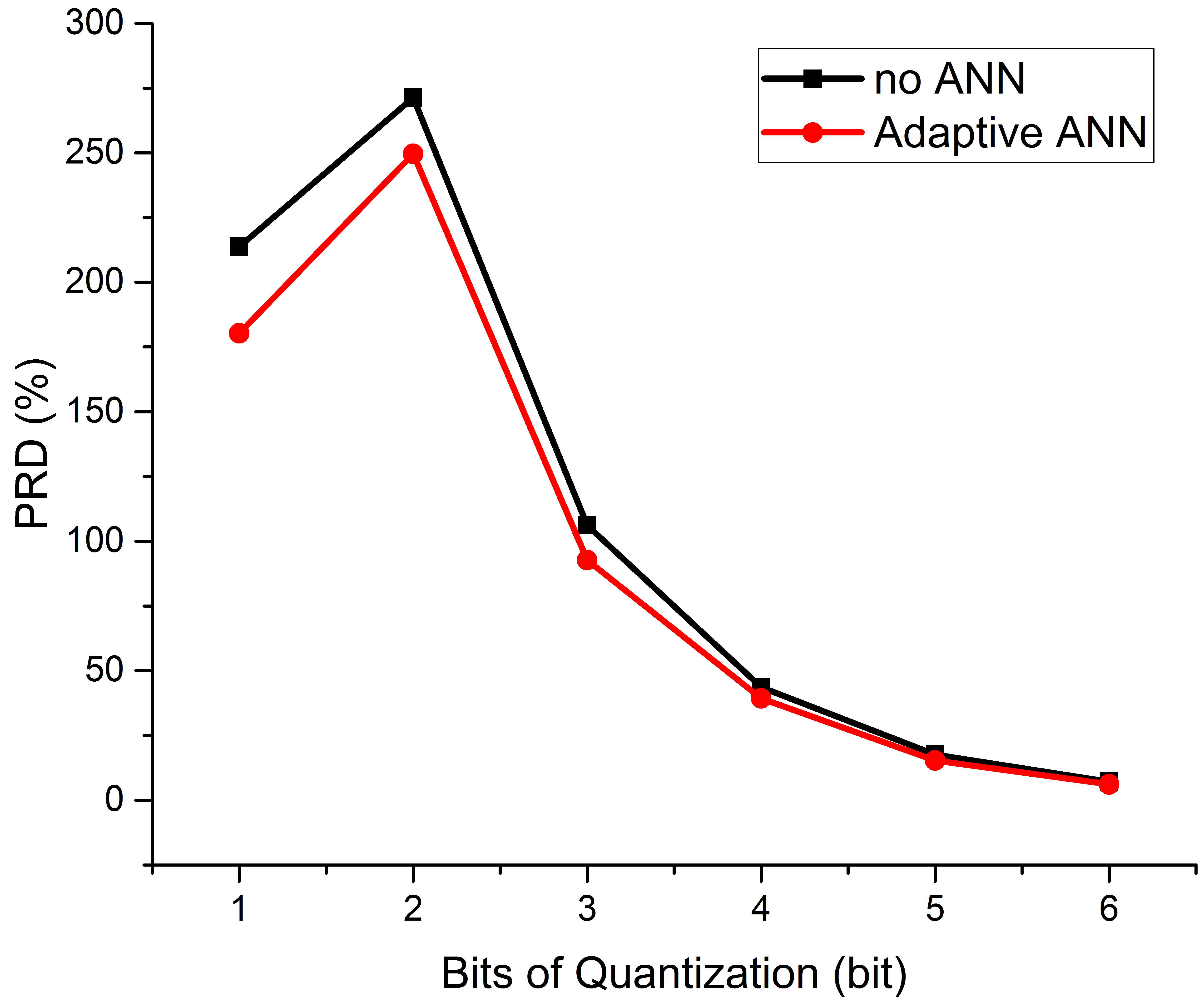
In order to examine the effect of the adaptive ANN, the PRD values with and without using the adaptive neural network were calculated under different quantization levels. As shown in Figure 5, the curve of the adaptive neural network was always below the non-neural network, indicating that the adaptive neural network can improve the results at each point and effectively reduce PRD. The improved performance of PRD2 to PRD1 was calculated using Equation (22). Table 3 compares the percentage reduction in the PRD value after using the adaptive neural network with that not using ANN, showing that there were 8.01% to 15.67% increases under different quantization bits.
These improvements are mainly attributed to the enrichment of information by ANN and the personalized model constructed through incremental learning. In this paper, the ANNc layer compressed the 80-point DCT coefficients into 16 points. This step used the automatic optimization feature of ANN to find a model that mapped 80 points of information to 16 points and reconstructed the signal as much as possible. In addition, due to the large difference among individual signals in SSVEP, the incremental learning method used in this paper utilized the adaptive characteristics of ANN and individual data for targeted training, which could improve the adaptation of the ANN model to an individual. Moreover, this could improve the degree of personalization and the quality of the compressed signal.
3.2. Influence of Non-Uniform Single Point Quantization on Results
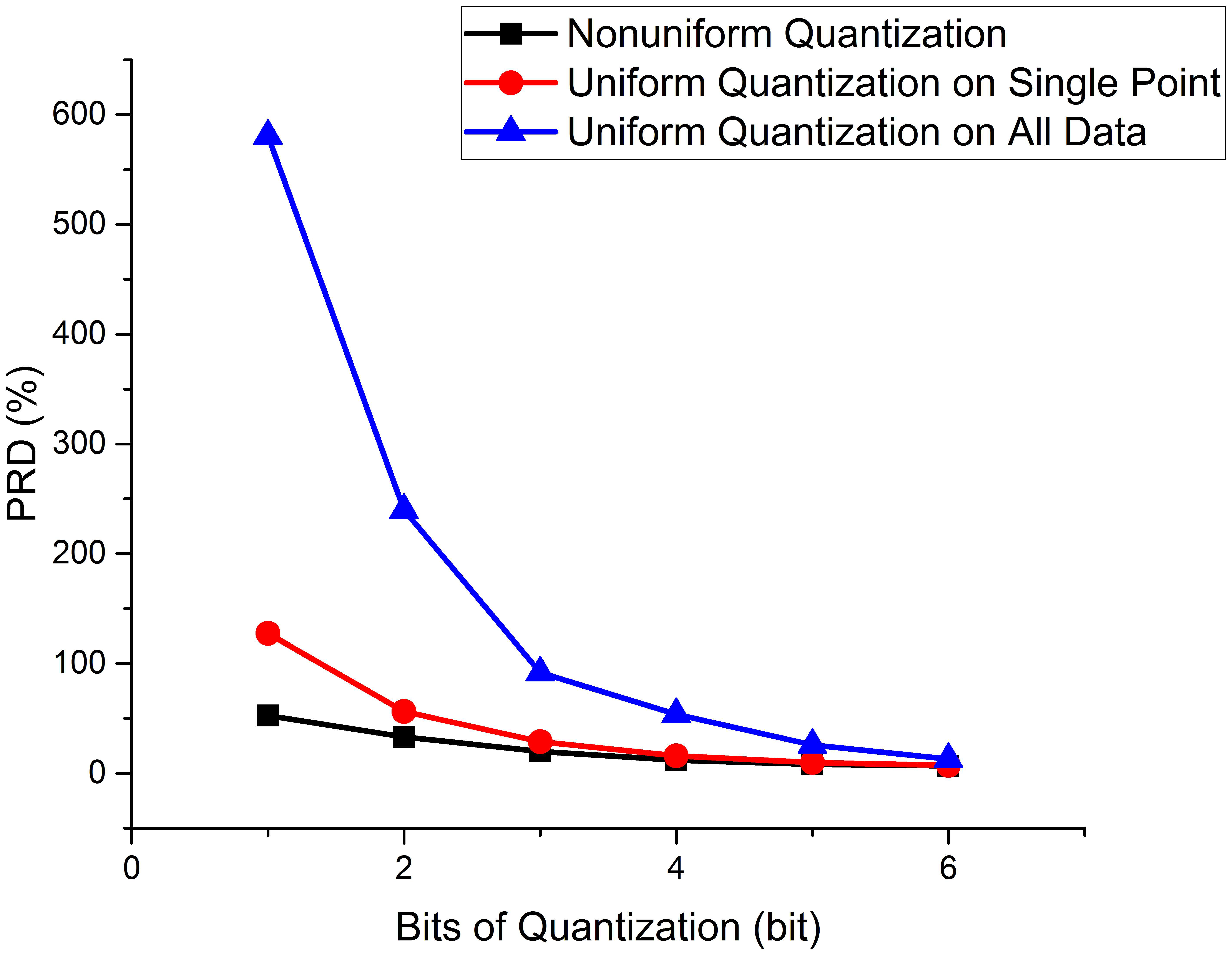
In the experiment, a separate quantification table was calculated for each DCT point of each sample to achieve the best quantification and reconstruction effect. In the traditional uniform quantization method, all the data are used for statistics, and the maximum and minimum values in the data are taken, and then the values are divided into equal-length intervals to obtain a uniform quantification table [28]. All points in an interval are quantized to the intermediate value of the interval. This quantification is not suitable for SSVEP because the DCT signal of SSVEP has different strengths and importance at different frequencies, and treating them all with the same quantization precision would lead to serious bias. In this paper, statistics were calculated separately for each frequency point to obtain a unique quantization table, and different frequency points used different quantization tables.
The effect was significantly improved by using the non-uniform quantization table proposed in this paper for every single point. As shown in Figure 6, the non-uniform single-point quantization PRD was smaller than the uniform quantization and uniform single-point quantization. The improvement of non-uniform quantization over the two uniform quantizations is shown in Table 4. At different bit quantization degrees, the PRD reductions ranged from 4.33% to 58.81% for single-point uniform quantization and improved by 46.32–90.98% for multi-point uniform quantization.
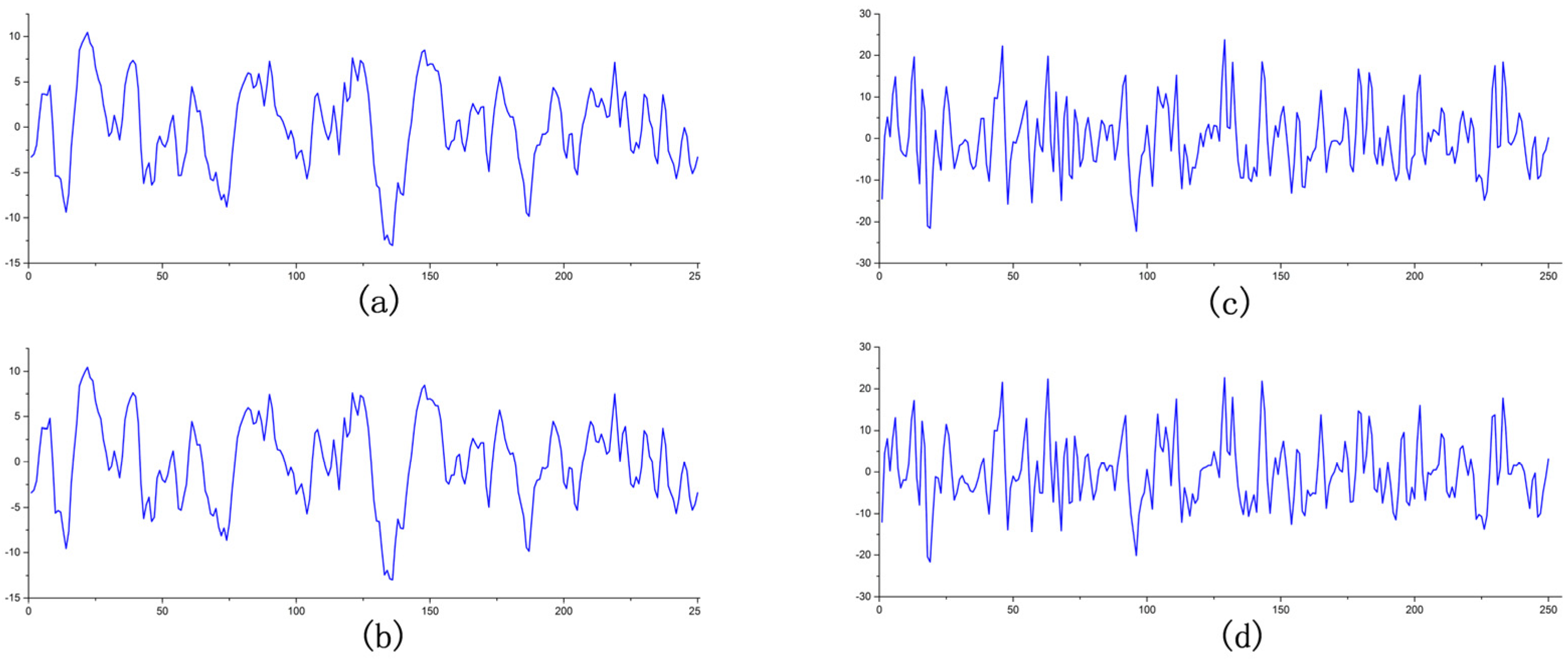
Figure 7 visualizes the effect of the reconstruction by comparing the same signal before and after compression. The first group is the signal of subject 44 in the dataset, where the quantization bit is 6 bits, CR is 7.95, and PRD is 2.84%. The second group is the comparison chart of subject 16, where the quantization bit is 3 bit, CR is 12.7, and PRD is 22.19%. The waveforms before and after compression are almost identical, with only slightly different amplitudes in detail, which are minor and within acceptable limits.
4. Discussion
This study proposes a method using adaptive ANN and non-uniform quantization for compression, which significantly improves signal quality compared to the non-ANN method and uniform quantization. Such an improvement is mainly attributed to specific analysis and statistics for specific signals. The adaptive ANN part is based on the general model obtained on the training set. Then, the individual experimental part of each sample is used to perform incremental learning to achieve an individualized model to improve the reconstruction accuracy for individuals.
The non-uniform quantization part considers individual differences and the differences of each frequency point. It combines the different amplitude distribution of frequency points to determine different quantization intervals according to statistical characteristics to obtain a better quantization effect when the number of quantization bits is equal.
We also computed the overall improvement in adaptive ANN and non-uniform quantization over the two uniform quantizations without ANN. As shown in Table 5, at different bit quantization degrees, the method in this paper showed a PRD reduction of from 11.65% to 61.50% for single-point uniform quantization without ANN, compared with multi-point uniform quantization without ANN, which showed a PRD decline of from 50.63% to 91.61%.
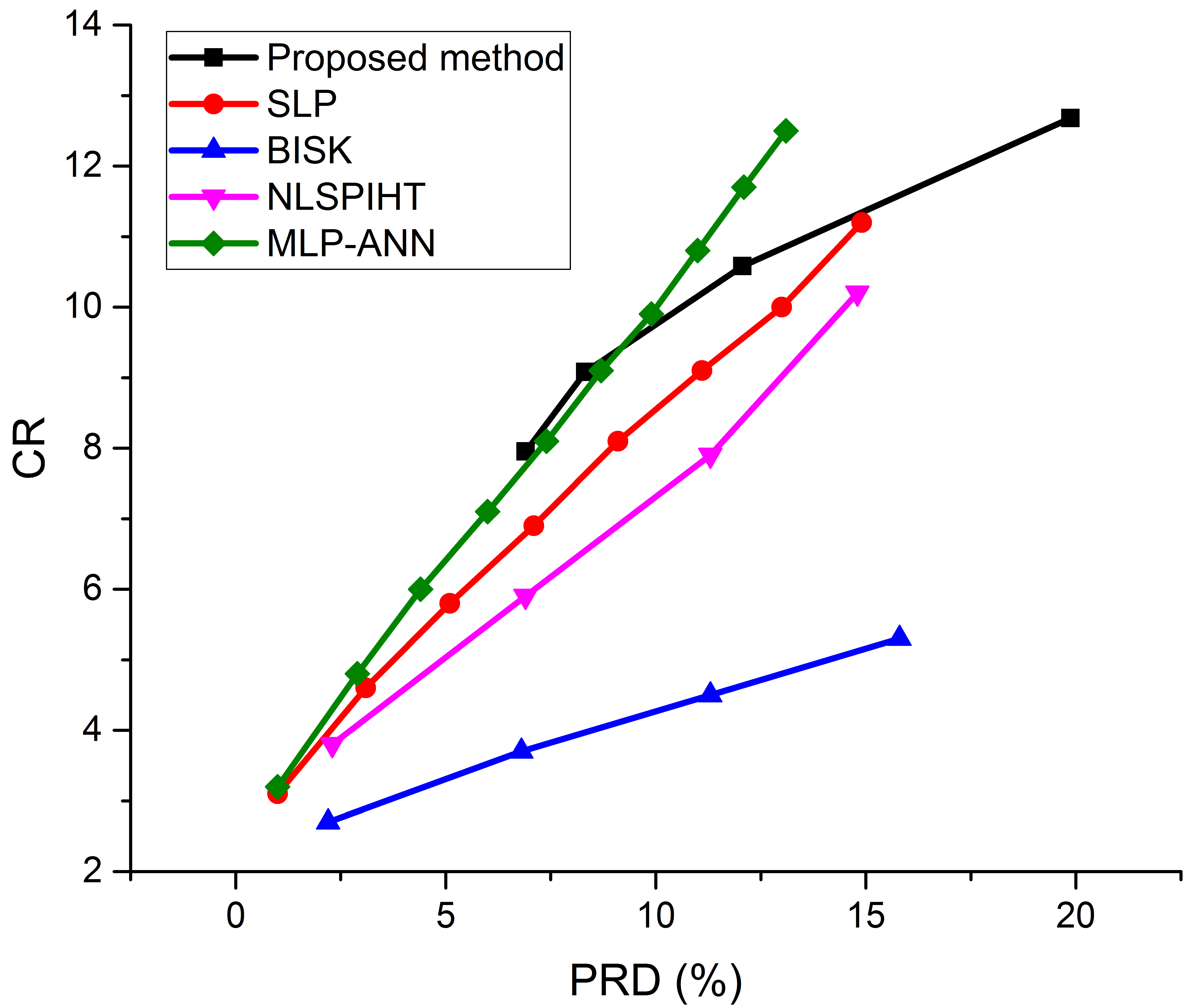
Figure 8 shows the comparison of the proposed method with other state-of-the-art methods (SLP [29], BISK [30], NLSPIHT [31], and MLP-ANN [28]). Our method has obvious advantages compared with SLP, NLSPIHT, and BISK. For MLP-ANN, this paper shows advantages in the range of a low compression rate and low PRD, but with the increase in CR, the PRD of the method proposed in this paper significantly increased. On the other hand, the method proposed in this paper saves one arithmetic coding module compared to MLP-ANN. Due to its application in wireless scenarios, the transmitting end of the compressed signal often has limited computing resources, and the calculation amount of the arithmetic coding module is very large [32]. The method in this paper provides a better performance at low compression ratios and a resource-saving option at high compression ratios.
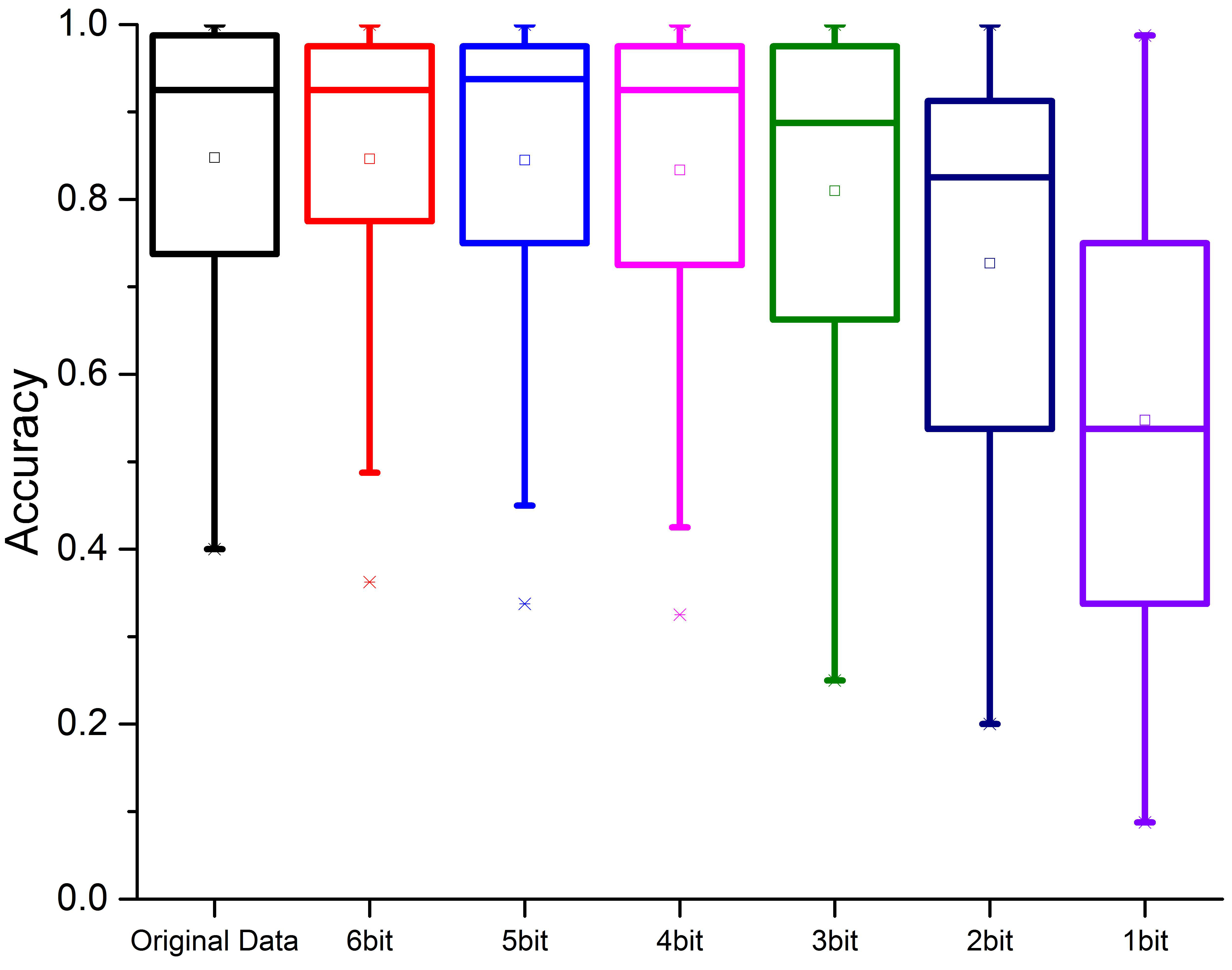
Since this paper proposes a compression optimization method for the specific application of SSVEP, the actual effect of the recovered data in SSVEP detection should be considered. In the application of SSVEP, the CCA algorithm and its variants are usually used for testing [13,14,33,34,35]. The eCCA algorithm used in this paper could provide an accuracy rate as a test result for each subject’s forty targets in each block of experiments. In the experiment, the decompressed data were tested by eCCA [14]. Since in ANN, the first two blocks of each subject were used as training sets to train the adaptive model, and the latter two blocks were used as test sets, in the eCCA test, the former two blocks of original data were used as training sets, and the latter two blocks of test sets were used to obtain accuracy rates. In this way, the impact of compressed data on the performance of SSVEP was evaluated. As shown in Figure 9, the results were not significantly affected when quantization bits were greater than 4. When using 3 bits for quantization, the accuracy rate decreased from 84.77% of the original data to 80.98%, a reduction of only 3.79%. The performance loss was not significant but fell within an acceptable range.
In our future work, to further improve the compression rate, we will consider the quantization of ANN weights to reduce the number of bits required for this part. In addition, the application of this framework outside SSVEP can also be studied, for example, in experiments on EEG signals that are sensitive to specific frequencies.
5. Conclusions
This paper proposes a compression–decompression framework for the application of EEG signals in SSVEP, in which adaptive ANN and non-uniform quantization methods are used to improve the compression effect. In this paper, an adaptive ANN and incremental learning were applied to the compression process to generate an exclusive ANN models for different subjects, which improved the degree of individualization of compression and the quality of compressed signals. Additionally, non-uniform quantization was also used in the quantization process, and corresponding quantization tables were adopted for different subjects and different signal positions, which improved the recovered signal quality after quantization. First, the DCT transform was used to concentrate the signal, and then the DCT coefficients were extracted and compressed using the adaptive ANN. To reduce the error, the difference between the restored value of ANN and the original value was calculated, and the compressed result was obtained via non-uniform quantization with statistical characteristics. After ANN decompressed the compression result, we could apply inverse quantization, error correction, and IDCT transform to reconstruct the signal. The method in this paper can effectively maintain the signal quality while ensuring a satisfying SSVEP performance after compression. When the accuracy rate decreased by 3.79%, the compression rate reached 12.7 times, which greatly reduced the amount of transmitted data and did not significantly impact use.
Author Contributions
Conceptualization, M.L.; methodology, S.Z., Y.Y., K.M. and B.R.; software, S.Z. and Y.Y.; validation, S.Z., K.M., B.R. and Y.Y.; formal analysis, S.Z.; investigation, S.Z.; resources, M.L.; data curation, S.Z. and B.R.; writing—original draft preparation, S.Z.; writing—review and editing, S.Z. and K.M.; visualization, S.Z.; supervision, S.Z. and M.L.; project administration, M.L.; funding acquisition, M.L. All authors have read and agreed to the published version of the manuscript.
Funding
This research received no external funding.
Institutional Review Board Statement
Not applicable for studies not involving humans or animals.
Informed Consent Statement
Not applicable for studies not involving humans.
Data Availability Statement
No new data were created or analyzed in this study. Data sharing is not applicable to this article.
Conflicts of Interest
The authors declare no conflict of interest.
References
- Landhuis, E. Neuroscience: Big brain, big data. Nature 2017, 541, 559–561. [Google Scholar] [CrossRef] [PubMed] [Green Version]
- Lalos, A.S.; Alonso, L.; Verikoukis, C. Model based compressed sensing reconstruction algorithms for ECG telemonitoring in WBANs. Digit. Signal Process. 2014, 35, 105–116. [Google Scholar] [CrossRef] [Green Version]
- Zhang, Z.; Jung, T.-P.; Makeig, S.; Rao, B.D. Compressed sensing of EEG for wireless telemonitoring with low energy consumption and inexpensive hardware. IEEE Trans. Biomed. Eng. 2012, 60, 221–224. [Google Scholar] [CrossRef] [PubMed] [Green Version]
- Gurve, D.; Delisle-Rodriguez, D.; Bastos-Filho, T.; Krishnan, S. Trends in Compressive Sensing for EEG Signal Processing Applications. Sensors 2020, 20, 3703. [Google Scholar] [CrossRef] [PubMed]
- Li, M.; He, D.; Li, C.; Qi, S. Brain-Computer Interface Speller Based on Steady-State Visual Evoked Potential: A Review Focusing on the Stimulus Paradigm and Performance. Brain Sci. 2021, 11, 450. [Google Scholar] [CrossRef]
- Tello, R.G.; Pant, J.K.; Mueller, S.M.; Krishnan, S.; Bastos-Filho, T.F. An Evaluation of Performance for an Independent SSVEP-BCI Based on Compressive Sensing System. In Proceedings of the World Congress on Medical Physics and Biomedical Engineering, Toronto, ON, Canada, 7–12 June 2015; pp. 982–985. [Google Scholar]
- Ingel, A.; Vicente, R. Information Bottleneck as Optimisation Method for SSVEP-Based BCI. Front. Hum. Neurosci. 2021, 15, 352. [Google Scholar] [CrossRef]
- Sharma, S.; Chaudhury, S.; Jayadeva. Block Sparse Variational Bayes Regression Using Matrix Variate Distributions With Application to SSVEP Detection. IEEE Trans. Neural Netw. Learn. Syst. 2022, 33, 351–365. [Google Scholar] [CrossRef] [PubMed]
- Zhang, Y.; Xie, S.Q.; Wang, H.; Zhang, Z. Data Analytics in Steady-State Visual Evoked Potential-Based Brain-Computer Interface: A Review. IEEE Sens. J. 2021, 21, 1124–1138. [Google Scholar] [CrossRef]
- Bonci, A.; Fiori, S.; Higashi, H.; Tanaka, T.; Verdini, F. An Introductory Tutorial on Brain–Computer Interfaces and Their Applications. Electronics 2021, 10, 560. [Google Scholar] [CrossRef]
- Bin, G.; Gao, X.; Yan, Z.; Hong, B.; Gao, S. An online multi-channel SSVEP-based brain–computer interface using a canonical correlation analysis method. J. Neural Eng. 2009, 6, 046002. [Google Scholar] [CrossRef] [PubMed]
- Chen, Y.; Yang, C.; Chen, X.; Wang, Y.; Gao, X. A novel training-free recognition method for SSVEP-based BCIs using dynamic window strategy. J. Neural Eng. 2021, 18, 036007. [Google Scholar] [CrossRef] [PubMed]
- Chen, X.; Wang, Y.; Gao, S.; Jung, T.-P.; Gao, X. Filter bank canonical correlation analysis for implementing a high-speed SSVEP-based brain–computer interface. J. Neural Eng. 2015, 12, 046008. [Google Scholar] [CrossRef] [PubMed]
- Chen, X.; Wang, Y.; Nakanishi, M.; Gao, X.; Jung, T.-P.; Gao, S. High-speed spelling with a noninvasive brain–computer interface. Proc. Natl. Acad. Sci. USA 2015, 112, E6058–E6067. [Google Scholar] [CrossRef] [Green Version]
- Ming, C.; Xiaorong, G.; Shangkai, G.; Dingfeng, X. Design and implementation of a brain-computer interface with high transfer rates. IEEE Trans. Biomed. Eng. 2002, 49, 1181–1186. [Google Scholar] [CrossRef]
- Belouadah, E.; Popescu, A.; Kanellos, I. A comprehensive study of class incremental learning algorithms for visual tasks. Neural Netw. 2021, 135, 38–54. [Google Scholar] [CrossRef] [PubMed]
- Delange, M.; Aljundi, R.; Masana, M.; Parisot, S.; Jia, X.; Leonardis, A.; Slabaugh, G.; Tuytelaars, T. A Continual Learning Survey: Defying Forgetting in Classification Tasks. IEEE Trans. Pattern Anal. Mach. Intell. 2021, 1. [Google Scholar] [CrossRef]
- Parisi, G.I.; Kemker, R.; Part, J.L.; Kanan, C.; Wermter, S. Continual lifelong learning with neural networks: A review. Neural Netw. 2019, 113, 54–71. [Google Scholar] [CrossRef] [PubMed]
- Liu, B.; Huang, X.; Wang, Y.; Chen, X.; Gao, X. BETA: A Large Benchmark Database Toward SSVEP-BCI Application. Front. Neurosci. 2020, 14, 627. [Google Scholar] [CrossRef] [PubMed]
- Lay, J.A.; Ling, G. Image retrieval based on energy histograms of the low frequency DCT coefficients. In Proceedings of the 1999 IEEE International Conference on Acoustics, Speech, and Signal Processing. Proceedings. ICASSP99 (Cat. No.99CH36258), Phoenix, AZ, USA, 15–19 March 1999; Volume 3006, pp. 3009–3012. [Google Scholar]
- Tjahyadi, R.; Liu, W.; Venkatesh, S. Application of the DCT Energy Histogram for Face Recognition. In ICITA 2004: Proceedings of the Second International Conference on Information Technology and Applications, Harbin, China, 9–11 January 2004; [Macquarie Scientific Publishing] IEEE: Sydney, Australia, 2012; pp. 314–319. [Google Scholar]
- Sriraam, N.; Eswaran, C. Context Based Error Modeling for Lossless Compression of EEG Signals Using Neural Networks. J. Med. Syst. 2006, 30, 439–448. [Google Scholar] [CrossRef] [PubMed]
- Sutanto, A.R.; Kang, D.-K. A Novel Diminish Smooth L1 Loss Model with Generative Adversarial Network. In International Conference on Intelligent Human Computer Interaction; Springer: Cham, Switzerland, 2021; pp. 361–368. [Google Scholar]
- Girshick, R. Fast r-cnn. In Proceedings of the IEEE International Conference on Computer Vision, Santiago, Chile, 7–13 December 2015; pp. 1440–1448. [Google Scholar]
- Zhonghai, W. Statistics-based Arithmetic of JPEG Quantization Table. J. Huazhong Agric. 2003, 22, 415–418. [Google Scholar]
- Zhu, F.; Jiang, L.; Dong, G.; Gao, X.; Wang, Y. An Open Dataset for Wearable SSVEP-Based Brain-Computer Interfaces. Sensors 2021, 21, 1256. [Google Scholar] [CrossRef] [PubMed]
- Wang, Y.; Chen, X.; Gao, X.; Gao, S. A Benchmark Dataset for SSVEP-Based Brain–Computer Interfaces. IEEE Trans. Neural Syst. Rehabil. Eng. 2017, 25, 1746–1752. [Google Scholar] [CrossRef] [PubMed]
- Hejrati, B.; Fathi, A.; Abdali-Mohammadi, F. A new near-lossless EEG compression method using ANN-based reconstruction technique. Comput. Biol. Med. 2017, 87, 87–94. [Google Scholar] [CrossRef] [PubMed]
- Sriraam, N. Correlation dimension based lossless compression of EEG signals. Biomed. Signal Process. Control 2012, 7, 379–388. [Google Scholar] [CrossRef]
- Srinivasan, K.; Dauwels, J.; Reddy, M.R. Multichannel EEG compression: Wavelet-based image and volumetric coding approach. IEEE J. Biomed. Health Inform. 2013, 17, 113–120. [Google Scholar] [CrossRef] [PubMed] [Green Version]
- Xu, G.; Han, J.; Zou, Y.; Zeng, X. A 1.5-D Multi-Channel EEG Compression Algorithm Based on NLSPIHT. IEEE Signal Processing Lett. 2015, 22, 1118–1122. [Google Scholar] [CrossRef]
- Sayood, K. (Ed.) Introduction to Data Compression; Elsevier: Amsterdam, The Netherlands, 2000. [Google Scholar]
- Nakanishi, M.; Wang, Y.; Wang, Y.-T.; Jung, T.-P. A comparison study of canonical correlation analysis based methods for detecting steady-state visual evoked potentials. PLoS ONE 2015, 10, e0140703. [Google Scholar] [CrossRef] [Green Version]
- Nakanishi, M.; Wang, Y.; Chen, X.; Wang, Y.-T.; Gao, X.; Jung, T.-P. Enhancing detection of SSVEPs for a high-speed brain speller using task-related component analysis. IEEE Trans. Biomed. Eng. 2017, 65, 104–112. [Google Scholar] [CrossRef] [PubMed]
- Lin, Z.; Zhang, C.; Wu, W.; Gao, X. Frequency recognition based on canonical correlation analysis for SSVEP-based BCIs. IEEE Trans. Biomed. Eng. 2006, 53, 2610–2614. [Google Scholar] [CrossRef] [PubMed]
Figure 1.
Schematic diagram of the SSVEP experiment: (a) The layout resembles a conventional keyboard with 26 alphabets, 10 numbers, and 4 non-alphanumeric keys (space, comma, dot, and backspace) aligned in 5 rows. The upper rectangle is designed to present the input character. (b) A subject is using the SSVEP system. (c) Schematic diagram of SSVEP data transmission. (d) Amplitude spectrum of SSVEP signal.

Figure 2.
System structure diagram.

Figure 3.
The mean of the squared values of the DCT coefficients.

Figure 4.
ANN schematic diagram.

Figure 5.
Influence of the presence or absence of adaptive neural network.

Figure 6.
Influence of different quantization methods on PRD.

Figure 7.
Comparison before and after signal compression: (a) EEG original signal of target 44. (b) Compressed reconstructed signal of target 44 (bits = 6, CR = 7.95, PRD = 2.84). (c) EEG original signal of target 16. (d) Compressed reconstructed signal of target 16 (bits = 3, CR = 12.7, PRD = 22.19).

Figure 8.
Comparison of the proposed method with SLP, BISK, NLSPIHT, and MLP-ANN.

Figure 9.
Influence of different quantization bits on SSVEP results.


Table 1.
The performance of different loss functions in the test set.
| L1 | L2 | Smooth L1 | ln | log10 | |
|---|---|---|---|---|---|
| MSE | 13.98 | 36.99 | 12.07 | 16.46 | 17.80 |
Table 2.
Quantization order correspondence.
| Bit | 1 | 2 | 3 | 4 | 5 | 6 |
|---|---|---|---|---|---|---|
| Quantization order | 2 | 4 | 8 | 16 | 32 | 64 |
| Compression ratio | 20.9974 | 15.8103 | 12.6783 | 10.5820 | 9.0806 | 7.9523 |
Table 3.
Improved performance of adaptive neural networks.
| Bit | 1 | 2 | 3 | 4 | 5 | 6 |
|---|---|---|---|---|---|---|
| Improved performance (%) | 15.67 | 8.01 | 12.68 | 9.91 | 13.15 | 13.74 |
Table 4.
The improvement in PRD by non-uniform quantization.
| Bit | 1 | 2 | 3 | 4 | 5 | 6 |
|---|---|---|---|---|---|---|
| Effect improvement compared with single-point uniform quantization (%) | 58.81 | 41.21 | 30.99 | 24.24 | 15.34 | 4.33 |
| Effect improvement compared with multi-point uniform quantization (%) | 90.98 | 86.10 | 77.62 | 77.93 | 68.99 | 46.32 |
Table 5.
Improvement in PRD using the overall algorithm.
| Bit | 1 | 2 | 3 | 4 | 5 | 6 |
|---|---|---|---|---|---|---|
| Effect improvement compared with single-point uniform quantization with non-ANN (%) | 61.50 | 44.64 | 35.53 | 29.82 | 21.45 | 11.65 |
| Effect improvement compared with multi-point uniform quantization with non-ANN (%) | 91.61 | 87.30 | 81.08 | 75.92 | 66.01 | 50.43 |
Publisher’s Note: MDPI stays neutral with regard to jurisdictional claims in published maps and institutional affiliations. |
© 2022 by the authors. Licensee MDPI, Basel, Switzerland. This article is an open access article distributed under the terms and conditions of the Creative Commons Attribution (CC BY) license (https://creativecommons.org/licenses/by/4.0/).
Share and Cite
MDPI and ACS Style
Zhang, S.; Ma, K.; Yin, Y.; Ren, B.; Liu, M. A Personalized Compression Method for Steady-State Visual Evoked Potential EEG Signals. Information 2022, 13, 186. https://0-doi-org.brum.beds.ac.uk/10.3390/info13040186
AMA Style
Zhang S, Ma K, Yin Y, Ren B, Liu M. A Personalized Compression Method for Steady-State Visual Evoked Potential EEG Signals. Information. 2022; 13(4):186. https://0-doi-org.brum.beds.ac.uk/10.3390/info13040186
Chicago/Turabian StyleZhang, Sitao, Kainan Ma, Yibo Yin, Binbin Ren, and Ming Liu. 2022. "A Personalized Compression Method for Steady-State Visual Evoked Potential EEG Signals" Information 13, no. 4: 186. https://0-doi-org.brum.beds.ac.uk/10.3390/info13040186
Note that from the first issue of 2016, this journal uses article numbers instead of page numbers. See further details here.