
Improving Performance and Quantifying Uncertainty of Body-Rocking Detection Using Bayesian Neural Networks


Department of Electrical and Computer Engineering, NC State University, Raleigh, NC 27606, USA
*
Author to whom correspondence should be addressed.
Information 2022, 13(7), 338; https://doi.org/10.3390/info13070338
Submission received: 26 May 2022
/
Revised: 1 July 2022
/
Accepted: 6 July 2022
/
Published: 12 July 2022
(This article belongs to the Special Issue Biomedical Signal Processing and Data Analytics in Healthcare Systems)
Abstract
:Body-rocking is an undesired stereotypical motor movement performed by some individuals, and its detection is essential for self-awareness and habit change. We envision a pipeline that includes inertial wearable sensors and a real-time detection system for notifying the user so that they are aware of their body-rocking behavior. For this task, similarities of body rocking to other non-related repetitive activities may cause false detections which prevent continuous engagement, leading to alarm fatigue. We present a pipeline using Bayesian Neural Networks with uncertainty quantification for jointly reducing false positives and providing accurate detection. We show that increasing model capacity does not consistently yield higher performance by itself, while pairing it with the Bayesian approach does yield significant improvements. Disparities in uncertainty quantification are better quantified by calibrating them using deep neural networks. We show that the calibrated probabilities are effective quality indicators of reliable predictions. Altogether, we show that our approach provides additional insights on the role of Bayesian techniques in deep learning as well as aids in accurate body-rocking detection, improving our prior work on this subject.
1. Introduction
Body rocking is one type of Stereotypical Motor Movement (SMM) observed in normal children (in medical literature referred to as “primary” cases) and in children presenting symptoms of distinct mental disorders (“secondary” cases). Such movements are normally involuntary and recurrent, sometimes nonrhythmic and purposeless. For secondary cases, SMM has partial overlap with developing disorders such as autism spectrum disorder (ASD), obsessive compulsive disorder (OCD), obsessive compulsive behavior (OCB), as well as self-destructive behavior (SDB), Tourette syndrome (TS), and attention deficit hyperactivity disorder (ADHD) [1,2]. Such repetitive behavior could be, but is not limited to, hand flapping, body rocking, or a combination of the two. Several possible triggers have been investigated for this behavior and some indications showed a link between such patterns with excitement and anxiety [3]. Body rocking has been shown to be common in blind infants [4] and may make maintaining social relationships more difficult [5]. A survey with college undergraduates has shown that self-reported body rocking is connected to General Anxiety Disorder, [6]. For primary cases of body rocking, the authors in [7] showed that habit reversal and differential reinforcement is beneficial for self-awareness and stopping of the movement, which is also summarized in Table 1 of [8].
Since medical research has shown potential for improvements through re-education, multiple efforts have been put together to identify and reliably characterize the occurrence of body rocking for both cases aforementioned, envisioning early diagnosis and self-awareness for behavior reversal.
Wearable sensors such as inertial measurement units (IMU), equipped with 3-axis accelerometers and gyroscopes, are appropriate for this purpose since they are non-invasive, lightweight, and may be placed on virtually any limb. However, signals collected among different individuals demonstrate variability in their properties that proposed algorithms for body-rocking detection have been challenging to deal with.
Real-time notification systems were implemented as part of a viability study [9] revealing an upper bound for real time notification but lacking good accuracy or detection results. Fast response and precision are key factors for accurate detection that engages the user to keep wearing the system. From our observations, we noticed that false negatives are more tolerable than false positives to minimize effects similar to “alert fatigue” [10,11], thus precision is potentially more important than recall. In order to address that, Bayesian neural networks (BNN) [12,13,14] could play an important role due to their capability of uncertainty quantification. Such networks have been shown to be versatile frameworks, which have been used for prosthesis applications [15,16], control and robotics [17], and activity recognition [18] to name a few. Uncertainty quantification could provide bounds to consider or discard a model’s prediction based on a desired trade-off between precision and recall. Therefore, BNNs can be used to not only to perform body-rocking detection but also to estimate the uncertainty associated with each prediction in order to prevent false positives. Consequently, the uncertainty quantification provided by BNNs can be a potential aid to avoid detecting repetitive activities that are not body rocking, therefore representing a key factor for continuous engagement of future users of wearable systems equipped with such technology. To the best of our knowledge, approaching body-rocking detection from the standpoint of primarily avoiding false positives, have not been attempted in the literature and it is an inherent limitation of the solutions available so far.
In this work, we present a framework for the detection of body-rocking activity. We take advantage of the uncertainty quantification provided by BNNs to stipulate a confidence for a given prediction. Our findings can be summarized as follows:
- With enough model capacity, our Bayesian framework provided better performance and was less sensitive to overfitting;
- Higher capacity alone did not consistently result on higher performance for a given model when compared to the Bayesian framework;
- Although transfer learning did not impact significantly the performance, it prevented the calibrated probability degradation as model complexity increased;
- The calibrated probability obtained from our Bayesian framework is an interpretable quantity that accurately represents the likelihood of correctness of the prediction of the specific dataset;
- Using the calibrated probability as a criterion for selecting reliable detection, we observe a clear improvement on precision with relatively low trade-off in other metrics (e.g., F1-score).
With that, we argue that reliable detection would be possible for real-time notification systems. The paper is organized as follows. Section 2 provides a literature overview of the detection of rocking motion. Section 3.1, presents the data collection system. The BNN framework, models used, pre-processing and evaluation strategies are included in Section 3.2, Section 3.4 and Section 3.5, respectively. Finally, the results and discussion are presented in Section 4 and Section 5, respectively.
2. Related Work
There exist three main methodologies in the literature for the detection of rocking motion: (1) using handcrafted features, (2) learning features from the data, or (3) a mix of the two.
The first methodology, handcrafted features, is the most popular. The study in [19] places wearable accelerometers on the chest as well as in front of a t-shirt collar for individuals with ASD presenting body-rocking behavior. A zero crossing method is applied on the time domain signals based on typical interval ranges and signal amplitudes between body-rocking motions where the best performance (84%) was obtained from the chest sensor. The study reported at [20] made use of recurrence plots which identifies similarities by means of Euclidean distance between accelerometer signals representing similar trajectories in a 3D phase space. The authors showed that this methodology is orientation invariant and claim resilience to disturbances caused by differences in amplitudes. Recurrence quantification analysis (RQA) was employed as a feature extraction method where characteristics such as amount of recurrences, determinism, and entropy were paired with a random forest (RF) algorithm to obtain classification accuracy of up to 86% on average. They also conducted an interesting analysis to find the best body location for the sensors. As a result, they found that the sensor placed on the torso contributed the most, based on the output of the RF algorithm. Additionally, using the signals from the torso provided the highest classification accuracy. This result corroborates the findings of [21]. Another approach relying on handcrafted features is the seminal work by [22] where the Stockwell transform, variance, mean difference between axes of entropy, and correlation coefficients were used as features to be classified for body-rocking detection with a support vector machine (SVM). Earlier approaches that are similar to the ones mentioned and based on handcrafted features can also be found in [21,23,24,25].
The second methodology in [26] is motivated by learning features from raw data in an end-to-end fashion. This work uses a similar deep learning approach to [27] by applying a convolutional neural network (CNN) to raw signals for feature extraction. This approach is applied to the dataset provided by [22] and their own, with simulated SMM and non-SMM activities. The extracted features were classified by long-short term memory (LSTM) recurrent neural networks (RNN), in a combination of knowledge transfer and ensemble learning to find the best performing model. In an earlier study [28], the same author developed a simpler method where instead of an LSTM for classification, an SVM was used and ensemble learning was not employed. Another very similar study by the same author tried the same configuration but with an LSTM [29], motivated by the argument that handcrafted features do not capture signal dependencies well. However, the author in [27] showed that handcrafted features still have value for SMM detection.
The third methodology is present in the work by [27]. It is a framework based on transfer learning with the support of CNNs. The CNNs were trained on time domain and frequency domain representations of the collected signals, where the frequency representations were extracted using the Stockwell transform as initially introduced to represent body-rocking signals in [22]. The transfer learning approach is justified by [27,30] due to the fact that data domains that share similar characteristics can enhance the ability of algorithms to learn and perform predictions on unknown data. Therefore, the CNNs are used to learn the time-frequency related information on SMM (body rocking, hand flapping, or simultaneous body, rocking and hand flapping) extracted from the dataset created and used by [22] and non-SMM related activities (such as walking, sitting, sitting down, standing and standing up) extracted from the PUC dataset [31]. The parameters learned with such training are later used as the transferred knowledge to an SVM classifier. They show this approach outperforming all contemporaneous state of the art methods [20,22,26] with accuracy and F1-score values capping on average at 98.29% and 93.66%, respectively.
Uncertainty quantification can be obtained by means of sampling or direct estimation recovering measures of uncertainty such as entropy, variance, mutual information, etc. Methods based on such approaches have been used for improving classification in activity recognition tasks [32,33,34], as well as eliminating predicted samples with high uncertainty [35]. In the context of multi-instance learning, uncertainty quantification has been used to improve instance level classifiers [36], and to aid active learning scheme to provide different levels of confidence about predicted samples for weak labelers (for the models under training) or strong ones (for the samples that had available labels) [37]. Model ensemble is one way of enabling uncertainty quantification in which such models could be even neural networks [38]. Modeling from a Bayesian approach allows one to estimate the model predicted samples distribution or posterior based on assumed prior distribution of the data. Although the prior assumptions may be misleading [39,40], there are works modeling an evolving prior for better estimation of the posterior [41].
As observed thus far, none of the main methods for body-rocking detection focused on reducing false positives, a factor that impacts a user’s ability to engage with a wearable system. Using uncertainty quantification for the purpose of eliminating bad predictions has not been proposed for the purpose of body-rocking detection to the best of our knowledge. Therefore, the BNN’s framework combines both the ability to screen bad detections and the ability to take advantage of the discriminative power of deep learning models (as discussed above).
3. Materials and Methods
3.1. Datasets
In this work, the public SMM dataset Electrodermal Activity Automated Quality Assessment (EDAQA) (preprocessed version can be found here: https://github.com/lsadouk/code_SMMs, accessed on 6 July 2022) [25] is used. This dataset was made available initially by [22], and the preprocessing and models by [27] are used as a benchmark. This dataset is split into two trials, Study 1 and Study 2. The sampling frequency of the IMU sensors is different from one trial to another, Study 1 is sampled at 60 Hz and Study 2 is sampled in 90 Hz. Additionally, the subjects are the same and the two trials are spaced out by two years. This public dataset will be referred to as EDAQA dataset.
The second dataset used in this study was collected by our group jointly with the Education Services for the Deaf and Blind (ESDB) of the North Carolina Department of Public Instruction under IRB 14046 [9], hence this dataset will be referred to as ESDB dataset (https://zenodo.org/record/5559169#.YqvpxtLMIUE, accessed on 6 July 2022). For the ESDB data, the 14 sessions were grouped into pairs to ease a granular analysis, hence ending with seven sessions. The characteristics of each dataset can be found in Table 1. In this work, the data coming from the wrist was not used since the performance obtained with it was not promising, as observed in our previous work [9]. Please note that since this dataset has only one subject, it can be used to analyze the performance of a personalized model rather than a population-level model.
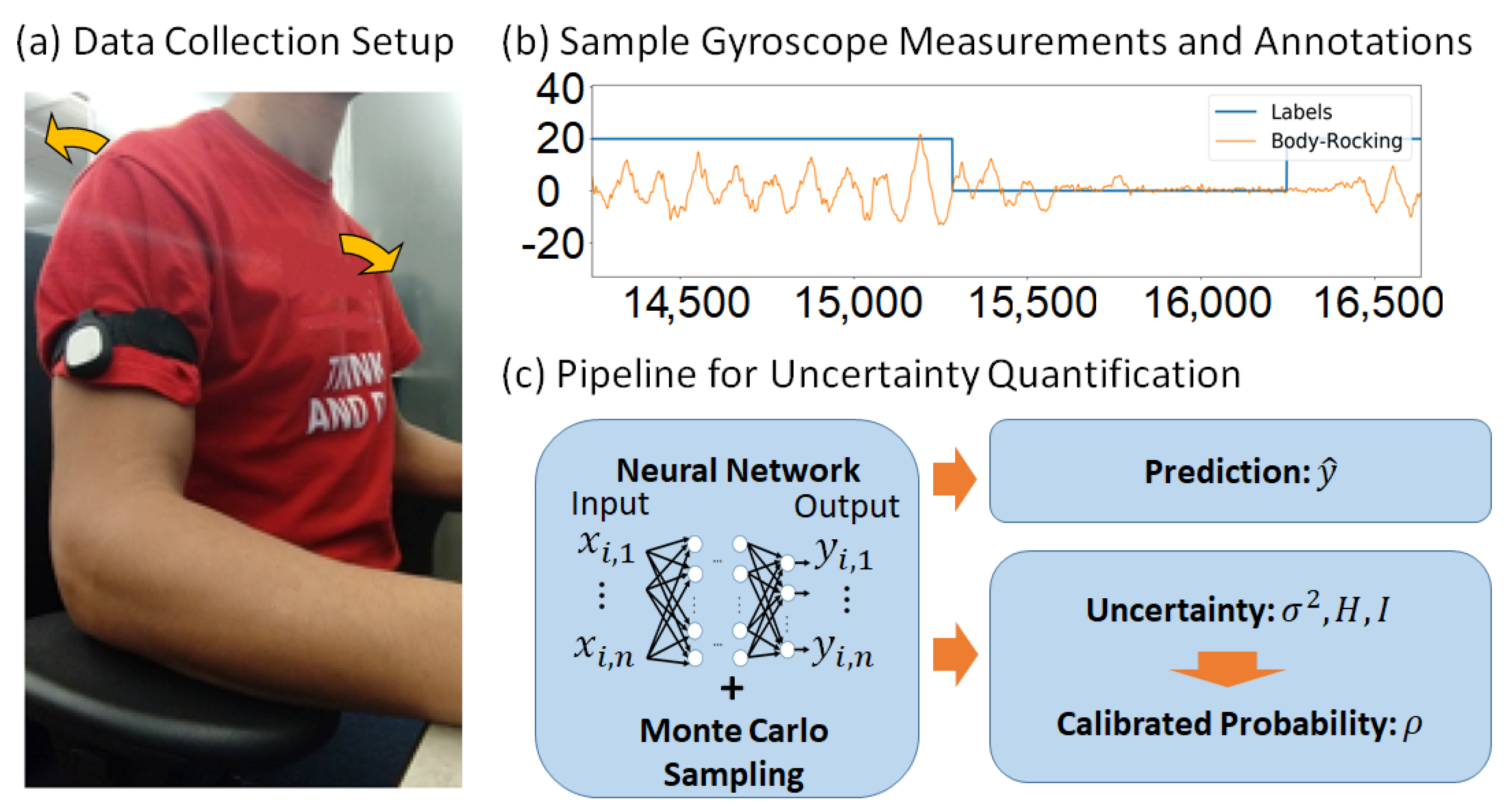
The ESDB dataset was collected using a Raspberry Pi Model 3, equipped with a touch-screen display to aid labeling the collected data in real time. The Mbientlab’s MetaMotionR IMUs (https://mbientlab.com/tutorials/MetaMotionR.html, accessed on 6 July 2022) were used. The IMU device contains an accelerometer, gyroscope, LED and a piezoelectric vibration generator. The software application has a UI for real-time data labelling implemented in Python 3.6. The operating system is the Rasbpian Stretch. The IMU streams data to the embedded system over bluetooth. The IMU sampling rate is 100 Hz. If the system were to be used for notifications, once a detection occurs, the vibration generator in the MetaMotionR device could be activated. A picture of the data collection procedure is shown in Figure 1.
3.2. Bayesian Neural Networks
Deep learning (DL) has shown incredible performance in different applications but it is still hard to analytically understand the internal nature of such models, which paradoxically may prevent further advancement of this technology. Model uncertainty has been used as a way to evaluate such models, offering a probabilistic interpretation of model’s intrinsic factors driving its performance. In particular, techniques such as dropout have been used to capture variability in deep learning models in a similar way to ensemble learning by randomly removing some network connections during training time [42].
For a while, it has been known that an infinite-depth neural network (NN) with a distribution established over its weights converges to a Gaussian process [12,42,43], while finite approximation to weights distributions has been attempted under the framework of Bayesian Neural Networks [12,13]. The authors in [14] showed that a neural network with arbitrary depth and non-linearities with dropout before its weights, as normally used in NNs, is a Bayesian approximation of a Gaussian process marginalized over its covariance parameters. This allows the characterization of the uncertainty due to intrinsic parameters to the model and due to its input data. Next, a brief introduction of the method used by [14] is presented, which shows how model uncertainty can be characterized while enabling model interpretability.
Let us consider the estimated output of a NN and the ground truth for an input with where each data point (, ) comes from the dataset , i.e., the sets of input and output, respectively. For our discussion, we will consider a NN with L layers of the form:
where is some activation function, are the NN weights and the vector of biases for each layer . A standard cost function often used for training of these networks (even when considering dropout) has the form:
where is a loss function, and the ’s are weight factors for regularization.
A deep Gaussian process (GP) is a model resulting of the hierarchical composition of GPs. A Gaussian process models a finite collection of its variables using a multivariate normal distribution with a defined covariance matrix function. Hence for a GP, the covariance matrix can be approximated using a variational distribution over each component of its spectral decomposition [14]. It is known that each hidden layer in a NN can be represented by one of the layers of a deep GP [14].
In this context, the predictive distribution of the deep GP model can be represented as:
for some precision hyper-parameter , where represent the normal Gaussian distribution with mean and covariance , and X and Y are the training set. Since the posterior is intractable, the authors in [14] show how to approximate it using variational inference. Such approximation is made by Monte Carlo Dropout sampling [14] and by minimizing the KL divergence between an approximating distribution and , as it will be shown next.
Now, let , with for , and , given some matrixes and probability as variational parameters. Note, that by using this argument we are in practice sampling the elements of . Let be the distribution over the matrix . We use the KL divergence between and the posterior as our objective for minimization, which (after some mathematical manipulation) can be expressed as:
Minimizing Equation (4) is equivalent to maximizing the log evidence lower bound [44], where the first term is equivalent to . Please note that Equation (4) would require integration over the entire space for the variable w, which does not scale well [45]. Therefore, it is shown next how the integral can be effectively approximated.
As shown in [14,46], the Monte Carlo approximation of the two terms in Equation (4) for the deep GP considered gives:
where are sampled from the distribution specified by by obtaining realizations of the Bernoulli distribution as it is made during the dropout process. By setting , we obtain an expression with similar form to Equation (2).
For the case of regression, and given enough training data (so the terms due to regularization of the weights and biases is negligible), we can approximate Equation (5) by [14]:
where is a variable that captures the observation noise for sample which is treated as another output of the NN.
Next, we discuss how to approximate the predictive distribution given a new sample point once the model has been trained. The distribution for the predicted value is [46]:
This distribution is approximated using a moment-matching technique by finding an estimate for the first two moments with the help of Monte-Carlo integration. The first moment approximation is obtained by the following:
where are obtained by drawing T samples from the distribution specified by . This expression is basically T averaged forward stochastic passes through the NN.
The second moment approximation is obtained by:
Hence the model’s predictive variance is obtained by:
which is the same as the sample variance of T forward passes through the NN plus the inverse of the model’s precision.
There are two types of uncertainties considered for quantification [45] (1) aleatoric uncertainty, which is the uncertainty associated with the data, (2) epistemic uncertainty, which is the uncertainty associated with the model [47] and usually can be explained by enough data [48]. For aleatoric uncertainty, there are two subtypes: heteroscedastic and homoscedastic. The first quantity is dependent on the data, while the second one assumes identical noise for all input samples.
Predictive entropy [49] measures the amount of uncertainty associated with a measurement. With the Monte Carlo dropout sampling, it is approximated as
Mutual information (MI) between the posterior over the weights and the prediction quantifies the uncertainty in the BNN’s output [50]. This measure is larger when the stochastic predictions are less stable, and it is calculated via:
Predictive entropy represents the effect of epistemic and aleatoric uncertainties. On the other hand, mutual information is a representation of the epistemic model uncertainty [47].
The regression aleatoric uncertainty is now extended to a classification task, by modeling the regression uncertainty of the logitvector—the output of the last layer before the Softmax activation function. A Gaussian distribution is placed over the logit vector as , where with as the NN. The expected log likelihood for each training sample is described as [15]:
where y is the ground truth label of x and c is the index for the ground truth label.
Since Equation (13) is analytically intractable, it is approximated by Monte Carlo integration. Denote , where follows a standard Gaussian distribution. The loss function becomes
where T is the number of Monte Carlo sampling iterations and is the class index of the logit vector [15]. The loss function in Equation (14) is the one that is going to be used later on in the experiments.
The uncertainty quantification relies on the estimation of the approximated predictive probability which for the classification case is shown by [48] as the output of softmax vector:
3.3. Probability Calibration
Assume a multi-class classifier with a prediction and corresponding predicted probability for an input x with representing the probability that the class label is correct. In this case, we would expect to match the empirical probability of this event. That is, a sufficient condition for calibration can be defined as
It is known that the predicted probability is not calibrated for neural networks, especially in the case of BNNs [45]. In this work, we employ the approach of Zhong et al. [15,51] of using the three uncertainties obtained with the BNN framework (i.e., the variance estimate of the prediction, the entropy and the mutual information) to find a map, say , from the uncertainties domain to a calibrated probability domain. Hence, a calibration function is desired such that produces calibrated probabilities, where U represents the three uncertainty measures from the BNN. In our framework, we used a neural network to approximate with architecture composed of three fully connected layers (FCN) with 32 (activation tanh) and 64 (activation tanh) neurons in the hidden layers and one neuron (activation sigmoid) for the output layer. Table 2 gives a summary of the equations so far.
3.4. The Models
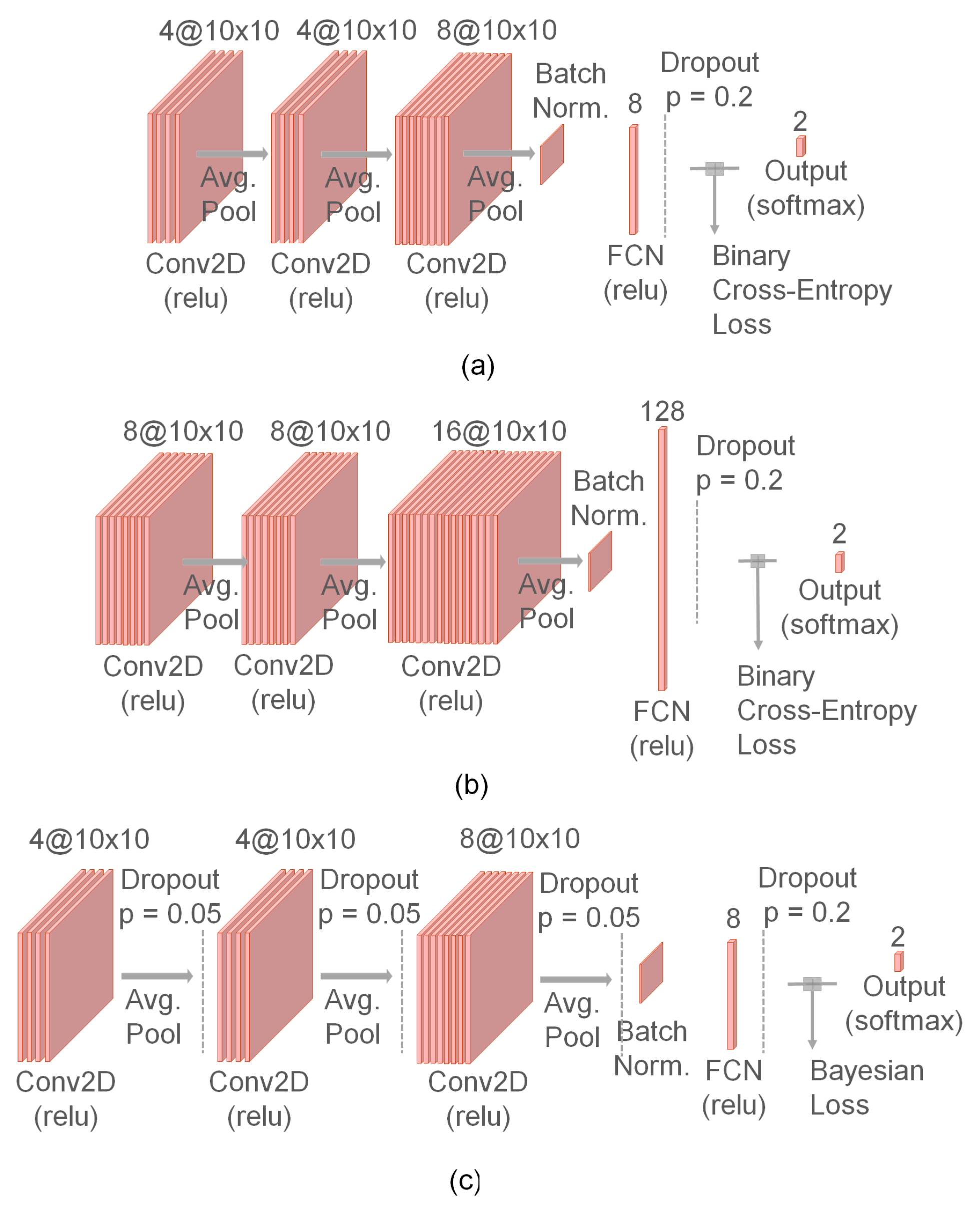
The Bayesian DL uncertainty quantification approach is applied to an end-to-end model, which together with Sadouk et al. [27] represents the state of the art for body-rocking detection in our assessment. We consider Rad et al. [26] as our baseline, who used a fully end-to-end deep learning approach for the same goal. For this implementation, we re-used most of the CNN pipeline developed by them (https://gitlab.fbk.eu/MPBA/smm-detection, accessed on 6 July 2022). This model is deeper than the one from [27] with 3 CNN layers of 4, 4, and 8 kernels, respectively. Each of these layers has filter sizes of 10 and stride of 1, the output of the CNN is flattened and passed through a batch normalization layer followed by an FCN with eight nodes, the logits are then dropped out with to generate a hot encoding output for body rocking and not-body-rocking status. For training this network, a cross-entropy loss function is used. A diagram of Rad’s architecture is shown in Figure 2a. This model will be referred to as Rad’s model or Rad’s approach and it represents the state of the art for end-to-end detection of body rocking in our assessment.
For a fair use of the Bayesian DL framework, we evaluate an additional model that is wider than the one aforementioned. The model will be referred to as WiderNet which is basically an upscaled version of Rad’s approach in terms of number of filters per layer. For instance, the model WiderNet 2× would be a three-layer CNN model, exactly as in Rad’s approach, but with 8, 8, and 16 filters per layer of size 10 each. Two variants of the models are created differing only in the number of nodes in their FCN. Therefore, the model “WiderNet 2×, FCN 128” has 128 nodes in its FCN as one can see in Figure 2b, thus the abbreviation “FCN” will be followed by the quantity of nodes. The use of a WiderNet is justified since Rad’s model is a narrow model (a few filters per layer) and may not display the advantages of the Bayesian approach since Rad’s shallower aspects do not contribute to the premises of Bayesian formulation; namely, the deeper/wider the model, the closer to a Gaussian process. To show that Wider models gain more benefits when using a Bayesian approach, the WiderNet will be upscaled and evaluated 2×, 4×, 8×, and 16× for comparison. Each upscaled version is going to be evaluated with the original Rad’s FCN (i.e., 8 nodes) and 128 nodes. Implementation is publicly available (https://github.com/rafa-coding-projects/Body-Rocking, accessed on 6 July 2022).
3.5. Dataset Pre-Processing and Evaluation Strategy
As mentioned earlier, we used the public EDAQA dataset and our ESDB dataset for analysis. The detailed characteristics of each dataset can be found in the preprint version of this manuscript (https://github.com/rafa-coding-projects/Body-Rocking, accessed on 6 July 2022). The models are evaluated in both datasets with the leave-one-subject-out (for the EDAQA dataset) or leave-one-session-out (for the ESDB dataset) strategies for training and testing. The training was performed for 45 epochs. For each subject left out, the procedure is repeated 10 times to account for additional variability in the training process.
For all models, the data were filtered by a Butterworth band-pass filter, segmented into windows of N samples for each axis (either three axes of gyro of accelerometer measurements), and trained end-to-end as described in the original work [26]. The window size is a moving window with .
For the Bayesian approach, the models had their original loss function replaced by the Bayesian loss (see Equation (14)), and dropout is added for each layer with probability 0.05. A diagram showing the additions of the Bayesian components to Rad’s model can be found in Figure 2c.
3.5.1. Transfer Learning for Model Improvement
As a comprehensively explored topic in statistics and DL literature [26,27], transfer learning (TF) is useful to take advantage of data coming from similar domains, consequently increasing model generalization capabilities. In the application of wearable sensors, transfer learning is especially useful to allow a model to work with sensors placed on different limbs.
In our particular scenario, we initially train the best performing model using the EDAQA data and later on we re-train the model on the ESDB dataset conserving most of its parameters. As explained before, the torso is the optimal location for body rocking, since it has minimal coupling with other repetitive activities that could be performed by other limbs. On the other hand, data coming from the arm has significant mechanical coupling with other activities, which makes it much more challenging to work with. For example, in a classroom environment, repeatedly taking folders from the student’s backpack to their desk would trigger a detector on the wrist but it may not on the chest. The transfer learning technique has been chosen as an aid to improve the model’s performance in the challenging (ESDB) arm data set.
3.5.2. Uncertainty Quantification as a Criterion for Choosing Reliable Predictions
We make use of the uncertainty quantification metrics as well as the calibrated probabilities generated by the Bayesian DL framework to develop a criterion to establish whether a prediction made by the model should generate a notification or not. More specifically, we will make use of a threshold on these quantities as a criterion for selection of a reliable detection. Entropy and MI were chosen to be reported since they were shown to be the most effective. We have not found any clear relationship between the predictions and other dispersion measures, such as estimated variance, inter-quantile ranges, coefficient of variation, etc. Finally, as mentioned in the introduction, excessive false positives can lead to alert fatigue. The trade-off between the distributions of correct and incorrect predictions will be analyzed as the threshold is changed.
3.5.3. Metrics
For the evaluation metrics, we focus on Area-Under-Curve (AUC) of the computed Receiver Operating Characteristic (ROC) curve and precision. The AUC is known to be less sensitive to oscillations in predictions and a good indicator for generalization, in contrast to other metrics such as accuracy. The other metrics reported are precision, recall, and F1-score. For the Bayesian approach, the metrics above are calculated using the model output specified by (15). The regular softmax output (as shown in Figure 2a,b) is for non-Bayesian models.
4. Results
4.1. Bayesian Approach Compared to Current Methods
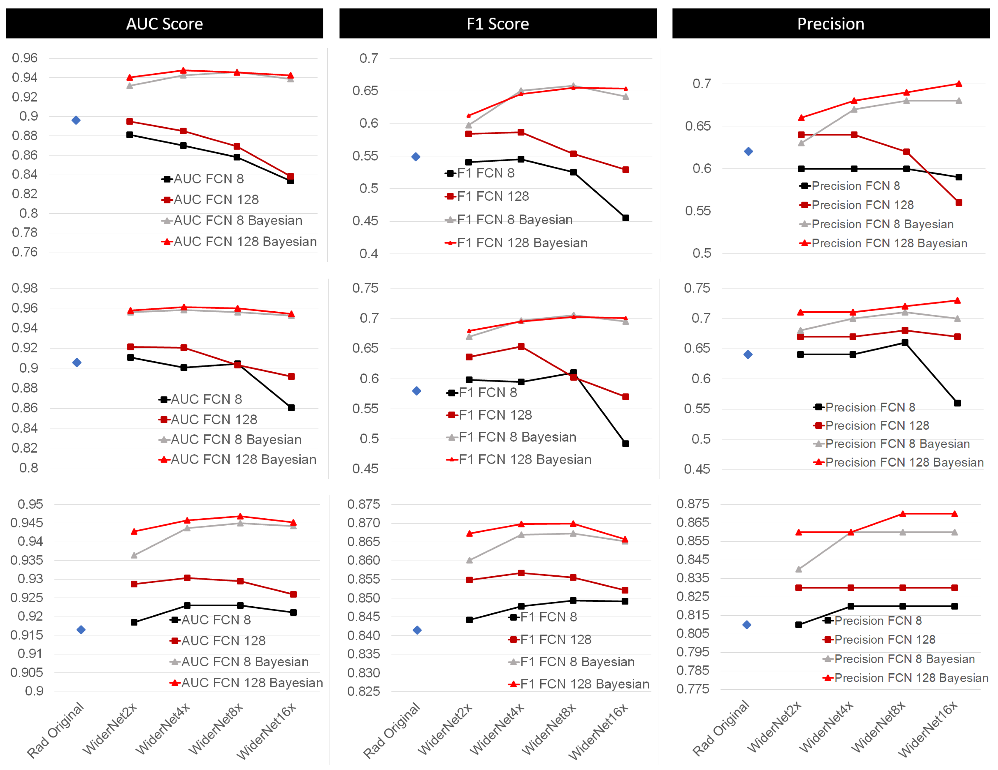
For the EDAQA Study 1 in Figure 3 top, one can observe that the AUC, and F1-score obtained by Rad’s approach is in general superior to the WiderNet models without a Bayesian approach (with a legend as “AUC FCN 8” and “AUC FCN 128”). By evaluating the curves for the AUC plot, one can observe that increased model complexity seems to be degrading the model’s performance, most likely due to overfitting. The Bayesian approach stands out as being superior to Rad’s approach by almost one standard deviation when using WiderNet 8× FCN 128. The figure also shows that the Bayesian approach does not require an aggressive increase on capacity of the architecture in order to perform better since WiderNet 2× already increases the AUC by 3%, all obtained AUC values are around 94% for the Bayesian approach.
We continue evaluating Study 1, but now for F1-score in Figure 3 top in the middle column. As expected, the performance degradation due to increase in capacity of non-Bayesian models is also reflected in their F1-score.
Furthermore, different improvements are obtained as the WiderNet’s capacity is increased, which is more noticeable than when analyzing the AUC. The F1-score for Bayesian approach increases from 61% to almost 66%. WiderNet 8× provided the highest F1-score of 65.8%, just slightly above WiderNet 8× FCN 128 with 65.5%, more than 10% compared to the F1-Score obtained with Rad’s approach of 54.9%. Precision is also further improved by the Bayesian approach from 62% with Rad’s model to reaching up to 70% with WiderNet 16× FCN 128. Therefore, for F1-score and precision, the Bayesian approach provided greater improvement than for AUC.
For EDAQA Study 2, the reader can refer to Figure 3 middle. The performance in this portion of EDAQA dataset is superior than the performance obtained in Study 1 as also shown in [27]. The same model degradation trend when increasing capacity observed in Study 1 is also present in Study 2 when considering non-Bayesian approaches. On the other hand, the WiderNet 8× provided an F1-score of 70% compared to 58% of Rad’s model, an improvement of 12%. The precision when using WiderNet 16× was at 73% and Rad’s model at 68%, an improvement of 5%.
Finally, for ESDB in Figure 3 bottom, one can observe a superior average performance by WiderNet variants in general when compared to Rad’s model. This happens although all AUC values are within a range of about 4%. Thus, considering AUC, one can see that widening Rad’s model provided improvements for the non-Bayesian approach of WiderNet 2× and 4× only. Increasing the model capacity any further degrades the AUC, as the non-Bayesian models variants WiderNet 8× and WiderNet 16× show, independently of how many nodes are placed in the FCN. The Bayesian approaches had an even higher performance since AUC improvements were observed until an increase in capacity of 8×. The models that had FCN 128 seem to be less sensitive to capacity increase. The FCN 128 Bayesian variants seem to have plateaued in terms of performance, leading us to believe that the framework has reached a limit in performance. Applying the Bayesian framework to Rad’s model slightly improved its AUC score from 92% to 93% while the Bayesian WiderNet 8× had 95%.
The results for WiderNet FCN 128 are averaged and summarized in Table 3. Finally, considering also AUC for model generalization as well as dealing with an imbalanced data, the up-scaled model WiderNet 8× FCN 128 seems to be the best performing one. In Figure 4, one can verify how AUC, and precision play a role between the best models and Rad’s.
4.2. Effect of Transfer Learning (TF)
We evaluated all Bayesian WiderNet FCN 128 variants using TF. It was observed that TF from the EDAQA to the ESDB dataset was not effective for Rad’s approach, it rather substantially decreased their performance. We noticed that Bayesian WiderNet models obtained better performance with TF than Rad’s model, but still slightly worse than training the models from scratch.
It is important to note that [27] obtained good results and improvements using TF from one subject to another. However, the same limbs were being used, while in our case, TF was attempted from torso data to right upper arm data. The sensing modalities are also different, since EDAQA dataset only uses an accelerometer, whereas in ESDB the body-rocking activity is more evident in the gyroscope data.
The transfer learning is accomplished by first training a Bayesian approach model from scratch on EDAQA Study 1, since from previous results, it seems to be a bit more challenging for the models than Study 2, the imbalance in that portion of EDAQA dataset is also less severe than in Study 2. Then, the first CNN layer and the FCN of the model are trained on ESDB data analogously as before, namely, with 35 epochs, using leave-one-subject out for the testing set and repeating this procedure 10 times for each subject.
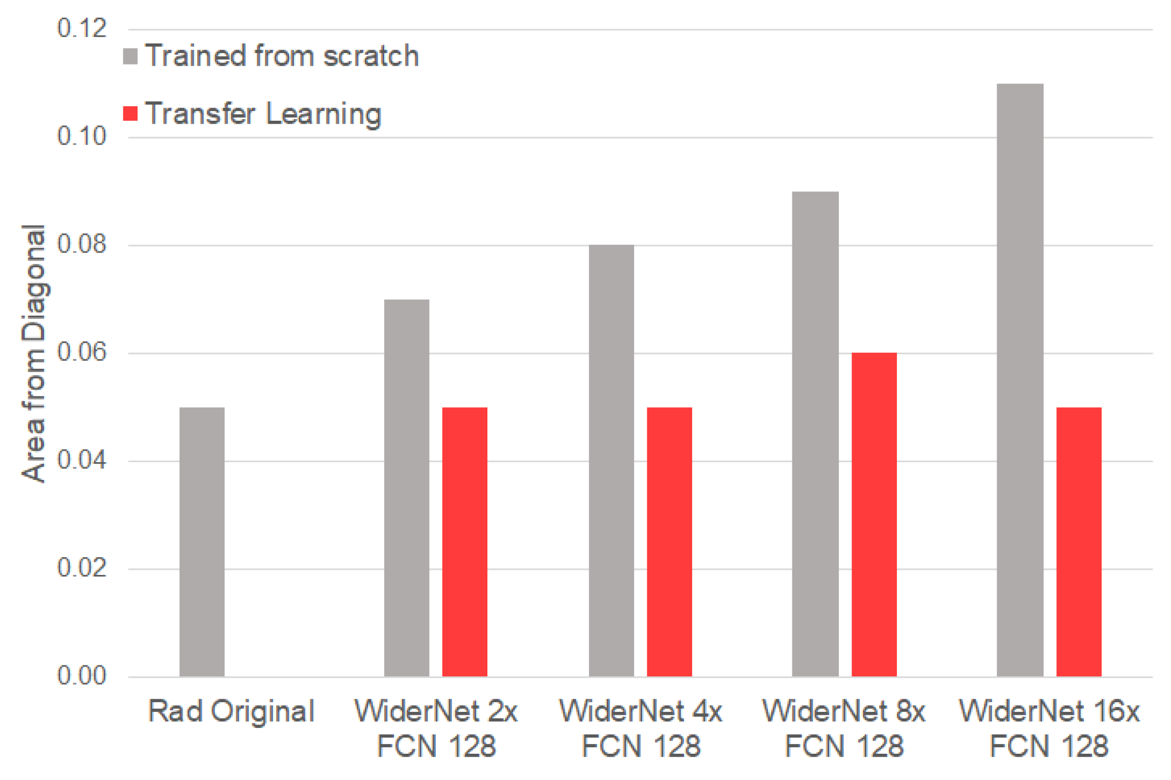
We also analyzed the reliability plots or calibration diagrams, which capture the correctness of the calibrated probability (as described in Section 3.3). The preprint version of this manuscript (https://github.com/rafa-coding-projects/Body-Rocking, accessed on 6 July 2022) contains one example of a reliability plot. The x-axis of the plots captures the mean calibrated probability value (i.e., which value of is predicted), and the y-axis corresponds to the fraction of positives in the dataset. Ideally, these numbers should match and the resulting curves should follow a diagonal line. To capture the offset from this ideal configuration, we report the Area From Diagonal (AFD), i.e., the area between the model curve and the diagonal. The AFD is reported for all WiderNet models with FCN 128 with and without TF in Figure 5. We observe that TF seems to help the Bayesian models to neutralize the effect of higher variability as the model capacity increases.
4.3. Uncertainty-Based Detection Selection
In this section, we explore the use of uncertainty as a criterion to select only predictions with high confidence. The Bayesian WiderNet 8×, FCN 128 model is used for this discussion since it is the model that provided the best overall performance among all models. The exploration is performed in the ESDB dataset only, since this is the focus of this manuscript for developing real-time notification systems.
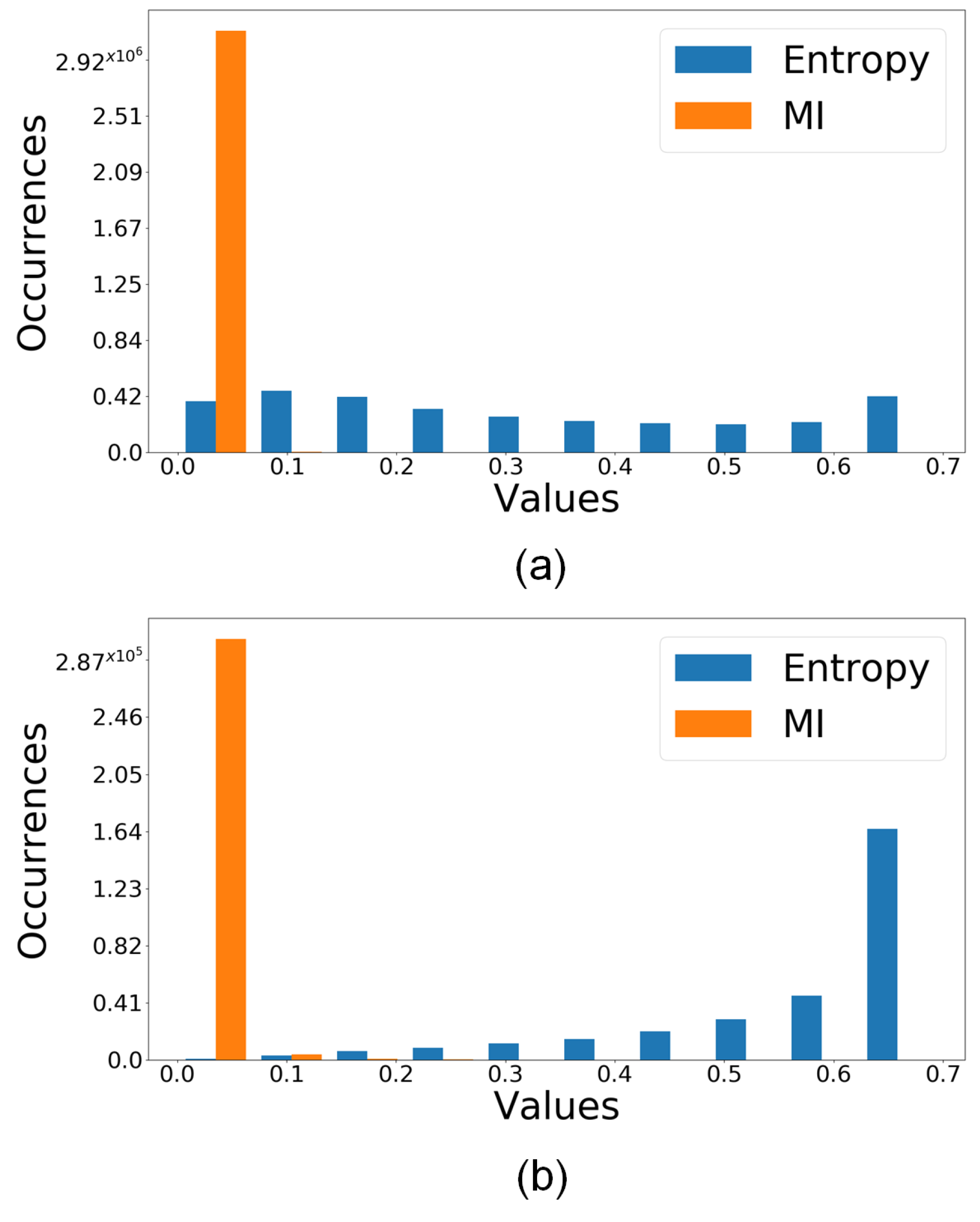
The distributions of the Entropy and MI measures of uncertainty for the correct and incorrect predictions are displayed in Figure 6.
One can observe that the distribution of incorrect predictions have a higher occurrence of entropy values greater than 0.4. One cannot tell much about a distinct pattern of MI since both groups have high concentration of values smaller than ; therefore, only entropy is used for the analysis detailed next. Rad’s model displays similar patterns.
We consider two uncertainty criteria for detection selection: (1) Setting positive detections with entropy above a specified threshold to be a negative (i.e., only keeping those detections with entropy that is low enough) and (2) Setting positive detections with calibrated probability below a specified threshold to be negative (i.e., only keeping those detection with calibrated probability that is high enough). Making use of the calibrated probability as a selection criteria is more desirable since the probability values can be more easily interpreted, and also because, as seen in the discussion below, it provides a better trade-off than using a single uncertainty measure. The goal is to use these criteria for selection of predictions that are truly reliable in order to avoid alarm fatigue.
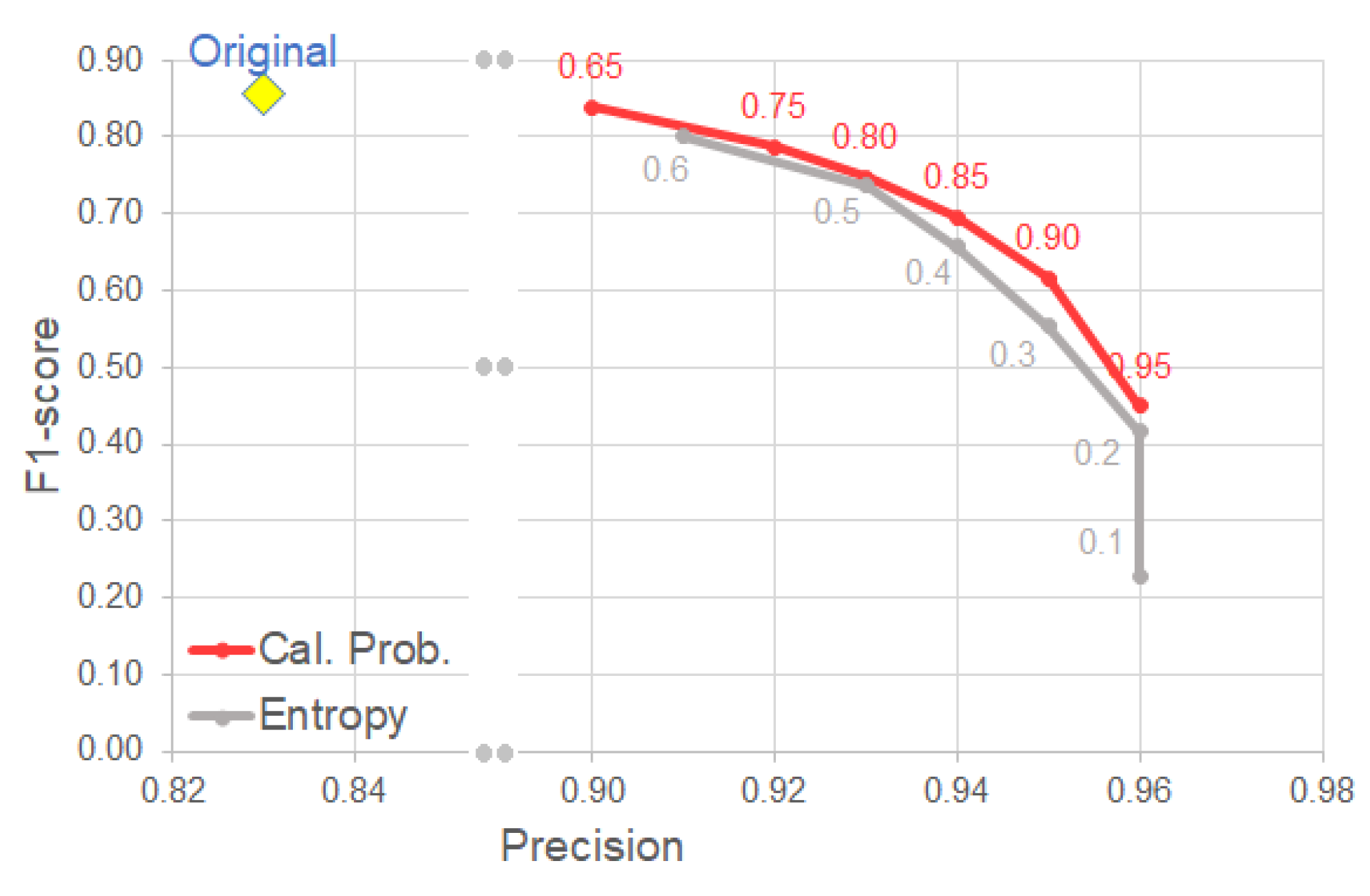
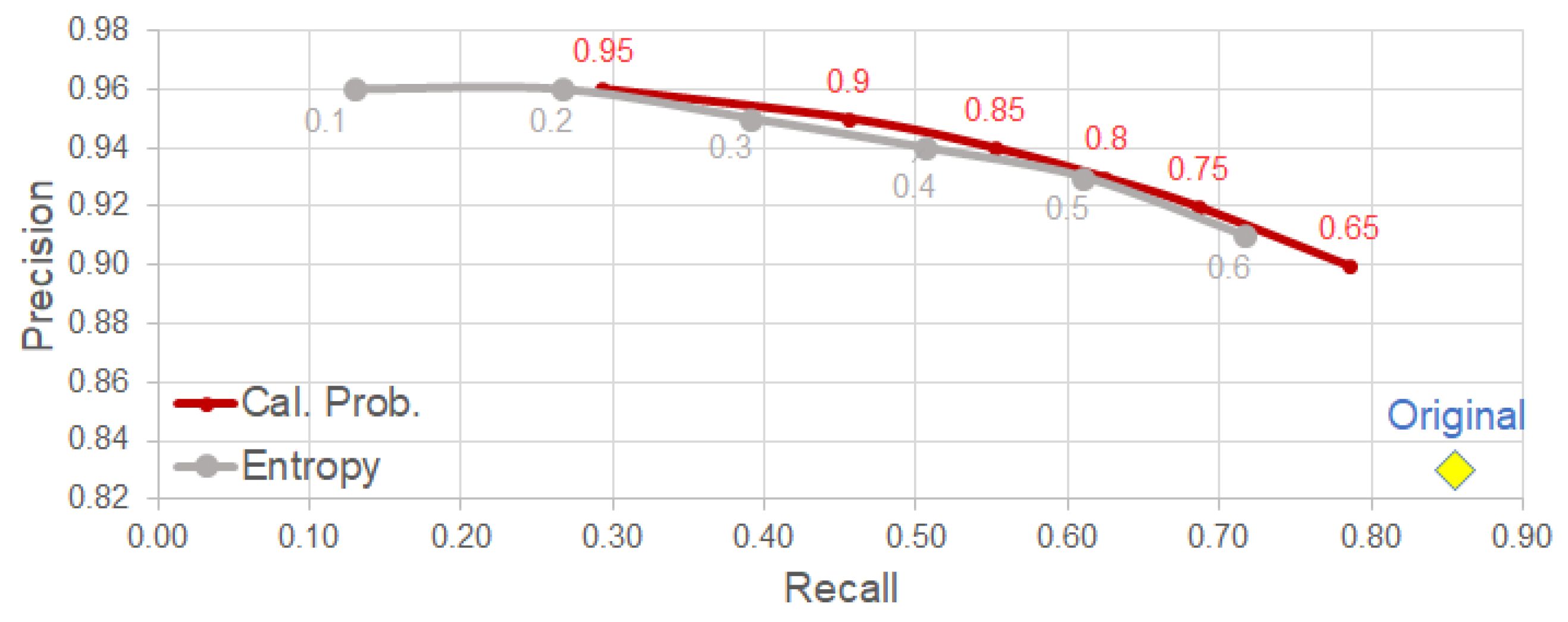
Figure 7 provides a visualization of the trade-off between F1-score and precision. Please note that the calibrated probability with a threshold of 0.65 yields a slight drop in the F1-score while increasing precision by 7%. This is a beneficial trade-off for our use case since that means that we can obtain more true positive detections without sacrificing the overall performance of the system. This degradation in F1-score was further explored in Figure 8 by exploring the impact in recall. We observe that for an improvement of 7% in precision, the degradation in recall was of around 6%.
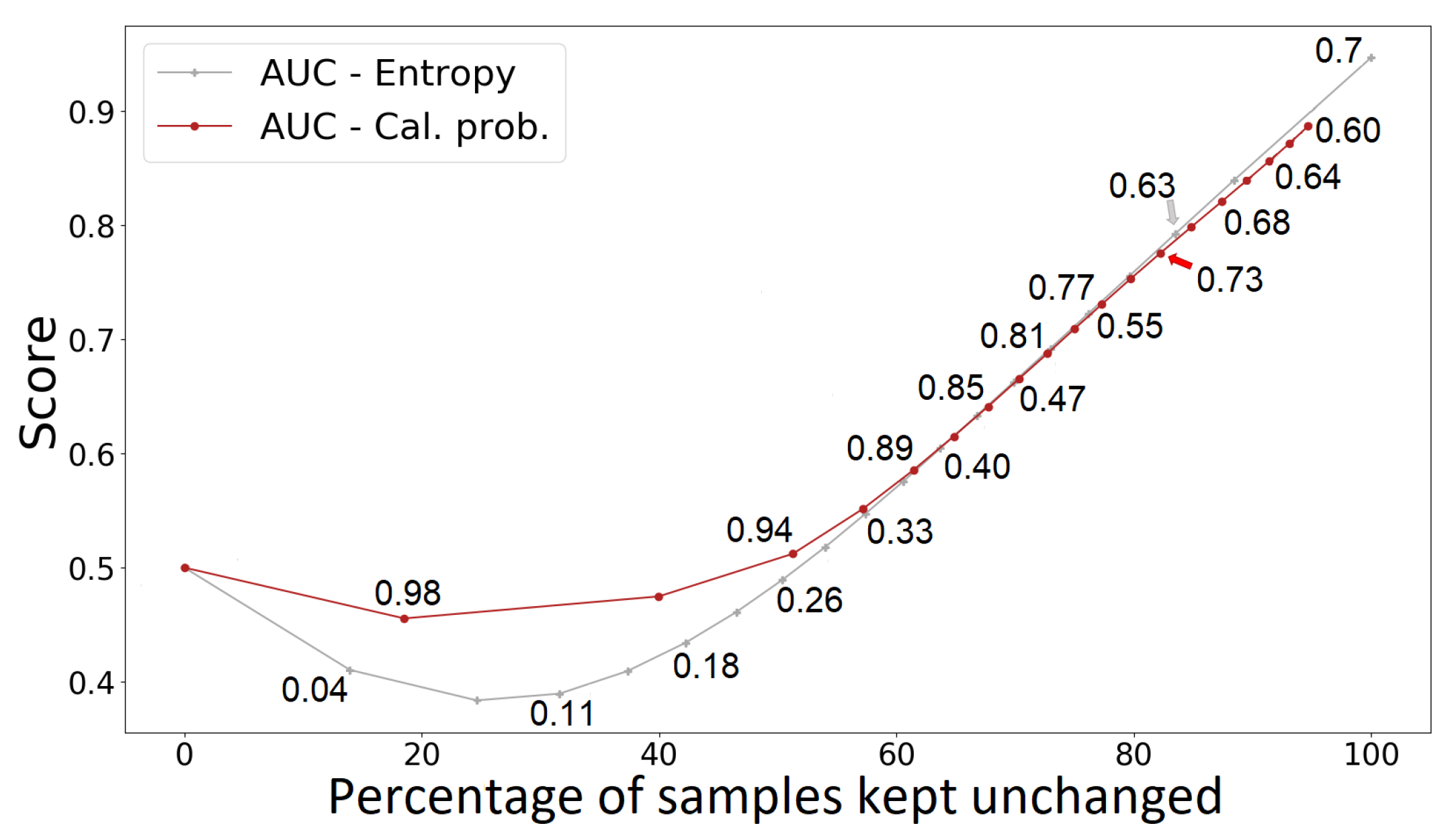
Since the proposed criteria rejects some of the original detections of the model, Figure 9 shows the trade-off between uncertainty threshold values and the percentage of samples that are kept unchanged (i.e., not set as negative prediction by the threshold criterion). We notice that for a percentage of samples kept unchanged higher than 60%, both criteria will provide similar AUC values. This plot supports our previous analysis, showing the impact of sample selection in metrics, such as precision and F1-score.
5. Discussion
BNNs improve performance beyond what is obtained by simply increasing model capacity. The first experiments show that the Bayesian approach presented a modest and inconsistent improvement to Rad’s approach, it improved the performance on Study 2 while it was slightly degraded for Study 1 (see Table 3). Increasing model complexity for EDAQA dataset degraded performance for non-Bayesian models, making a case for possible overfitting. For WiderNet, the performance was enhanced in general when considering the Bayesian variants. One possible explanation is that applying the Bayesian framework on a model has a regularization effect [52], which for a model with lower capacity, such as Rad’s model, results in lower performance. It is important to note that the AUC improvements for Bayesian approach were insensitive to further increases in capacity, leading us to believe that the framework has reached a limit on its performance. Additionally, it is interesting to note that for the EDAQA dataset, the precision increases with larger Bayesian models whereas it decreases for larger non-Bayesian models. It is important to note that according to [53], a DL model approaches a Gaussian process as the number of layers of the DL model goes to infinity. Another important aspect to bring to the discussion is that as shown by [54] a sufficient deep and wide model can even fit corrupted data since DL models have enough capacity to model very complex and even noisy data. However, based on the observations so far, we have some evidence that the WiderNet model had benefited from the Bayesian approach, showing that not only deeper models benefit from such an approach but also widerones. It also shows that model capacity alone did not extract the “full potential” of the model. Additionally, the Bayesian approach gives us a relatively computationally cheap way of obtaining uncertainties from model predictions. One could argue that a simpler ensemble could also provide the same benefit, but based on our previous work [9] we observed that random forests for example does not perform well for this dataset (and thus we used an SVM); therefore, a DL approach was chosen for this work.
Transfer learning reduces model variability. The evidence provided in Section 4.2 supports a claim which has an intuitive appeal: a model that has learned a similar domain will provide less variability when being retrained. An interesting unfolding of this result could be used to investigate the impact in model generalization, which we leave as future work.
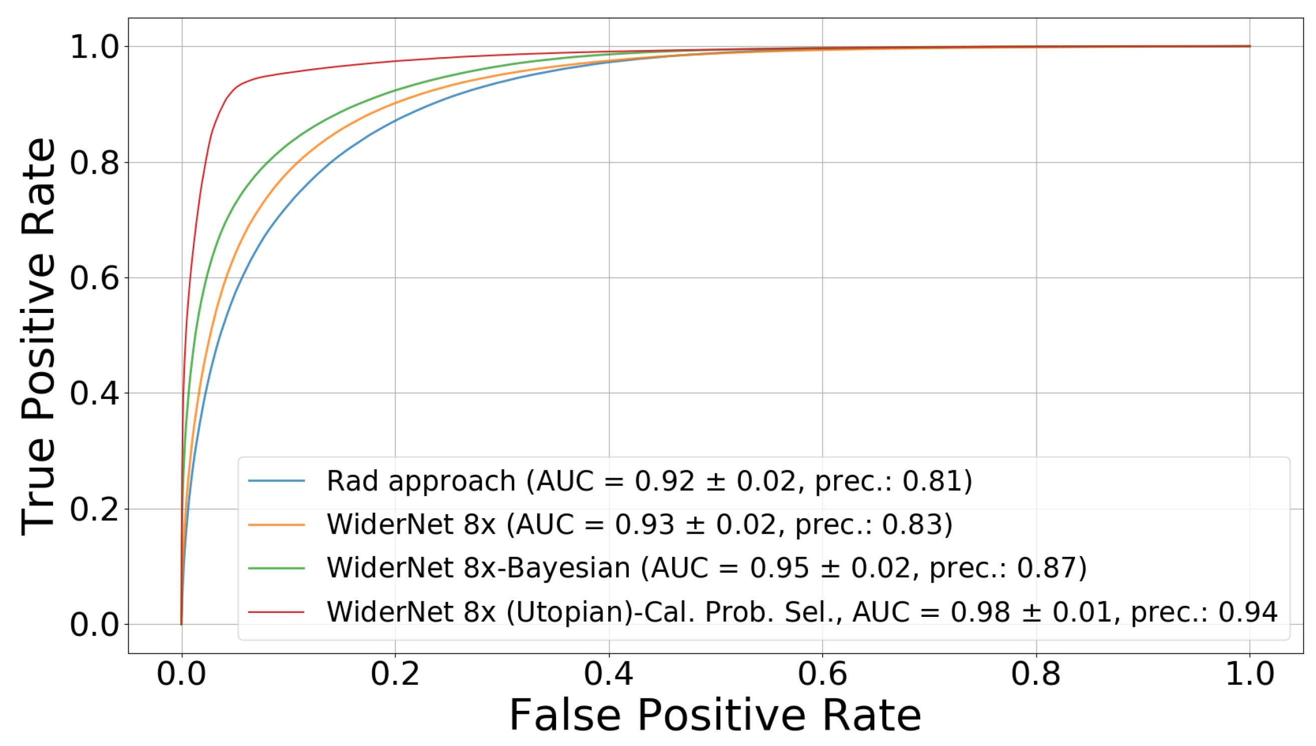
The calibrated uncertainty can serve as a prediction quality indicator.Section 4.3 shows that calibrated probability provides slightly better improvements in precision for choosing good predictions. To further illustrate that, we computed the ROC when removing the samples (and associated ground truth values) that do not meet the selection criterion and obtained an AUC of 98%. Although this represents an unrealistic scenario, we have evidence that the remaining samples are in very close agreement with their respective ground truth values. Revealing that the uncertainty-based thresholding really eliminates predictions with “poor quality”. Figure 10 illustrates this case by adding the new curve to former Figure 4.
Limitations and Future Work. This study and proposed pipeline have some limitations worth discussing. (1) Runtime. To produce the ensemble of predictions for uncertainty quantification, several predictions are necessary which require more computational power than for a single prediction. Thus, this is a constraint to be taken into consideration when implementing such methods in real time. However, a Ubuntu desktop with an CPU 3.7 GHz, 64 GB of RAM and a GPU GeForce GTX 1080 Ti takes 3 ms per inference for the Bayesian approach and 9 s for non-Bayesian, about 32 times more. Although this comparison was made on a desktop, implementing a deep architecture with Bayesian approach for real-time processing on an embedded device is viable as we showed in our previous work [51] with an architecture more complex than the ones presented in this manuscript. However, a clinical study should be considered with several subjects wearing a wearable system running the pipeline proposed in this work. With that, the shortcomings of the method in terms of comfort and effectiveness could be assessed. (2) Dataset size. Although we used a public dataset with six subjects, as noted in Section 3.1, we only evaluated uncertainty quantification results on the data with one subject. Repeating such evaluations on the EDAQA dataset could bring extra insights in future work. Additionally, expanding the ESDB dataset could potentially bring further insights into transfer learning between different subjects since the domain of EDAQA did not provide many performance improvements to the domain of ESDB what could be due to noise in EDAQA or simply lack of domain similarity. (3) Further Fine-Tuning of Pipeline. The results obtained from the pipeline can be potentially improved using a validation set and further tuning the parameters of the models, which is left for future work. (4) Prior sensitivity analysis. We have not comprehensively explored different priors for this work, but we acknowledge their importance in obtaining accurate posteriors depending on the size of the data.
The study of impact of different priors on body-rocking detection using BNN could be potentially interesting in future work. However, it is expected that priors should not have a big impact on performance for large datasets. (5) Fixed dropouts probability. We acknowledge that better results have been obtained in the literature using BNNs with dropout by learning the dropout probability during model training. Therefore, the performance showed in this manuscript could be potentially increased with such aid in a future work.
6. Conclusions
In this work, a comprehensive comparative study of methods to classify the body-rocking activity was presented. The methods were evaluated in light of a Bayesian approach. It was observed that a shallower model tends to not take advantage of the Bayesian approach. Additionally, the Bayesian approach was shown to provide superior performance benefits when applied to higher capacity models, as demonstrated by simple networks that were wider than the baseline model, which we called WiderNet. Although the experiments show this tendency, we acknowledge that more evaluations with other deeper and wider models, as well as other datasets, are needed in order to isolate the capacity effect v.s. Bayesian approach. Assuming precision as a better metric than F1-score for body-rocking classification, the calibrated probability and estimated entropy turned out to be useful criteria to establish a “reliable level” for model predictions, significantly improving the model’s precision, reducing the amount of false positives, and making the case to use such methods for real-time detection.
Bayesian DL is still a growing research area for which new insights are being shared. We foresee that the performance observed in this paper can be further improved by not only comprehensively evaluating deep architectures, but also exploring the effects of different priors for body-rocking classification and new ways of obtaining posteriors. The work of [55], for example, condensed a series of justifications for the use of cold posteriors on top of the fact that there is theoretical and experimental evidence that posterior predictive can be better than point estimators and that model averaging, in general, provide robust prediction. They show that cold posteriors improve the predictions of Stochastic Gradient-Monte Carlo Markov Chain-based ensembles, which could also bring benefits for body-rocking classification. Although there are claims in the literature showing that the deep learning architectures have so much capacity that they can even fit in corrupted data [54], we intend to show that the Bayesian approach does improve the predictions. Although we do not explore the impact of the prior in the predictions, we recognize its crucial role for accurate estimations of the posterior, as shown by [39,40,56]. Applications such as body-rocking detection can largely benefit from the constant new outcomes from Bayesian DL. In order to make “live" body-rocking detection using viable BNNs, a clinical study evaluating user feedback for real-time detection and uncertainty threshold adjustment should be conducted, with devices equipped with real-time BNNs, which we leave as future work.
Author Contributions
Conceptualization, R.L.d.S., B.Z. and E.L.; Data curation, E.L.; Formal analysis, R.L.d.S. and E.L.; Funding acquisition, E.L.; Investigation, R.L.d.S., B.Z. and E.L.; Methodology, E.L.; Project administration, E.L.; Resources, E.L.; Software, R.L.d.S. and Y.C.; Supervision, E.L.; Validation, R.L.d.S.; Visualization, R.L.d.S.; Writing—original draft, R.L.d.S.; Writing—review & editing, B.Z., Y.C. and E.L. All authors have read and agreed to the published version of the manuscript.
Funding
This work is supported by the National Science Foundation (NSF) under awards CNS 1552828 and IIS 1915599.
Institutional Review Board Statement
The study was conducted according to the guidelines of the Declaration of Helsinki, and approved by the Institutional Review Board 14046.
Informed Consent Statement
Informed consent was obtained from all subjects involved in the study.
Data Availability Statement
All data were presented in main text.
Conflicts of Interest
The authors declare no conflict of interest.
References
- Czapliński, A.; Steck, A.J.; Fuhr, P. Tic syndrome. Neurol. Neurochir. Pol. 2002, 36, 493–504. [Google Scholar] [PubMed]
- Singer, H.S. Stereotypic movement disorders. Handb. Clin. Neurol. 2011, 100, 631–639. [Google Scholar] [PubMed]
- Mahone, E.M.; Bridges, D.D.; Prahme, C.; Singer, H.S. Repetitive arm and hand movements (complex motor stereotypies) in children. J. Pediatr. 2004, 145, 391–395. [Google Scholar] [CrossRef] [PubMed]
- Troester, H.; Brambring, M.; Beelmann, A. The age dependence of stereotyped behaviours in blind infants and preschoolers. Child Care Health Dev. 1991, 17, 137–157. [Google Scholar] [CrossRef]
- McHugh, E.; Pyfer, J.L. The Development of Rocking among Children who are Blind. J. Vis. Impair. Blind. 1999, 93, 82–95. [Google Scholar] [CrossRef]
- Rafaeli-Mor, N.; Foster, L.G.; Berkson, G. Self-reported body-rocking and other habits in college students. Am. J. Ment. Retard. 1999, 104, 1–10. [Google Scholar] [CrossRef]
- Miller, J.M.; Singer, H.S.; Bridges, D.D.; Waranch, H.R. Behavioral therapy for treatment of stereotypic movements in nonautistic children. J. Child Neurol. 2006, 21, 119–125. [Google Scholar] [CrossRef]
- Subki, A.; Alsallum, M.; Alnefaie, M.N.; Alkahtani, A.; Almagamsi, S.; Alshehri, Z.; Kinsara, R.; Jan, M. Pediatric Motor Stereotypies: An Updated Review. J. Pediatr. Neurol. 2017, 15, 151–156. [Google Scholar] [CrossRef]
- Da Silva, R.L.; Stone, E.; Lobaton, E. A Feasibility Study of a Wearable Real-Time Notification System for Self-Awareness of Body-Rocking Behavior. In Proceedings of the 2019 41st Annual International Conference of the IEEE Engineering in Medicine and Biology Society (EMBC), Berlin, Germany, 23–27 July 2019; pp. 3357–3359. [Google Scholar]
- Wang, X.; Gao, Y.; Lin, J.; Rangwala, H.; Mittu, R. A Machine Learning Approach to False Alarm Detection for Critical Arrhythmia Alarms. In Proceedings of the 2015 IEEE 14th International Conference on Machine Learning and Applications (ICMLA), Miami, FL, USA, 9–11 December 2015; pp. 202–207. [Google Scholar]
- Eerikäinen, L.M.; Vanschoren, J.; Rooijakkers, M.J.; Vullings, R.; Aarts, R.M. Reduction of false arrhythmia alarms using signal selection and machine learning. Physiol. Meas. 2016, 37, 1204–1216. [Google Scholar] [CrossRef]
- Hinton, G.E.; Neal, R.M. Bayesian Learning for Neural Networks; Springer: Berlin/Heidelberg, Germany, 1995. [Google Scholar]
- MacKay, D.J.C. A Practical Bayesian Framework for Backpropagation Networks. Neural Comput. 1992, 4, 448–472. [Google Scholar] [CrossRef]
- Gal, Y.; Ghahramani, Z. Dropout as a Bayesian approximation: Representing model uncertainty in deep learning. In Proceedings of the International Conference on Machine Learning, New York, NY, USA, 19–24 June 2016; pp. 1050–1059. [Google Scholar]
- Zhong, B.; Silva, R.L.D.; Li, M.; Huang, H.; Lobaton, E. Environmental Context Prediction for Lower Limb Prostheses with Uncertainty Quantification. IEEE Trans. Autom. Sci. Eng. 2020, 18, 458–470. [Google Scholar] [CrossRef]
- Zhong, B.; Huang, H.; Lobaton, E. Reliable Vision-Based Grasping Target Recognition for Upper Limb Prostheses. IEEE Trans. Cybern. 2020, 52, 1750–1762. [Google Scholar] [CrossRef]
- Thakur, S.; van Hoof, H.; Higuera, J.C.G.; Precup, D.; Meger, D. Uncertainty Aware Learning from Demonstrations in Multiple Contexts using Bayesian Neural Networks. In Proceedings of the 2019 International Conference on Robotics and Automation (ICRA), Montreal, QC, Canada, 20–24 May 2019; pp. 768–774. [Google Scholar] [CrossRef] [Green Version]
- Akbari, A.; Jafari, R. Personalizing Activity Recognition Models Through Quantifying Different Types of Uncertainty Using Wearable Sensors. IEEE Trans. Biomed. Eng. 2020, 67, 2530–2541. [Google Scholar] [CrossRef]
- Gilchrist, K.H.; Hegarty-Craver, M.; Christian, R.P.K.B.; Grego, S.; Kies, A.C.; Wheeler, A.C. Automated Detection of Repetitive Motor Behaviors as an Outcome Measurement in Intellectual and Developmental Disabilities. J. Autism Dev. Disord. 2018, 48, 1458–1466. [Google Scholar] [CrossRef]
- Grossekathöfer, U.; Manyakov, N.V.; Mihajlovic, V.; Pandina, G.; Skalkin, A.; Ness, S.; Bangerter, A.; Goodwin, M.S. Automated Detection of Stereotypical Motor Movements in Autism Spectrum Disorder Using Recurrence Quantification Analysis. Front. Neuroinform. 2017, 11, 9. [Google Scholar] [CrossRef] [Green Version]
- Min, C.H.; Tewfik, A.H.; Kim, Y.; Menard, R. Optimal sensor location for body sensor network to detect self-stimulatory behaviors of children with autism spectrum disorder. In Proceedings of the 2009 Annual International Conference of the IEEE Engineering in Medicine and Biology Society, Minneapolis, MN, USA, 3–6 September 2009; pp. 3489–3492. [Google Scholar]
- Goodwin, M.S.; Haghighi, M.; Tang, Q.; Akçakaya, M.; Erdogmus, D.; Intille, S.S. Moving towards a real-time system for automatically recognizing stereotypical motor movements in individuals on the autism spectrum using wireless accelerometry. In Proceedings of the 2014 ACM International Joint Conference on Pervasive and Ubiquitous Computing, Seattle, WA, USA, 13–17 September 2014. [Google Scholar]
- Goodwin, M.S.; Intille, S.S.; Albinali, F.; Velicer, W.F. Automated detection of stereotypical motor movements. J. Autism Dev. Disord. 2011, 41, 770–782. [Google Scholar] [CrossRef]
- Min, C.H.; Tewfik, A.H. Automatic characterization and detection of behavioral patterns using linear predictive coding of accelerometer sensor data. In Proceedings of the 2010 Annual International Conference of the IEEE Engineering in Medicine and Biology, Buenos Aires, Argentina, 31 August–4 September 2010; pp. 220–223. [Google Scholar]
- Albinali, F.; Goodwin, M.S.; Intille, S.S. Recognizing stereotypical motor movements in the laboratory and classroom: A case study with children on the autism spectrum. In Proceedings of the 11th International Conference on Ubiquitous Computing, Orlando, FL, USA, 30 September–3 October 2009. [Google Scholar]
- Rad, N.M.; Kia, S.M.; Zarbo, C.; van Laarhoven, T.; Jurman, G.; Venuti, P.; Marchiori, E.; Furlanello, C. Deep learning for automatic stereotypical motor movement detection using wearable sensors in autism spectrum disorders. Signal Process. 2018, 144, 180–191. [Google Scholar]
- Sadouk, L.; Gadi, T.; Essoufi, E.H. A Novel Deep Learning Approach for Recognizing Stereotypical Motor Movements within and across Subjects on the Autism Spectrum Disorder. Comp. Int. Neurosc. 2018, 2018, 7186762. [Google Scholar] [CrossRef] [Green Version]
- Rad, N.M.; Furlanello, C. Applying Deep Learning to Stereotypical Motor Movement Detection in Autism Spectrum Disorders. In Proceedings of the 2016 IEEE 16th International Conference on Data Mining Workshops (ICDMW), Barcelona, Spain, 12–15 December 2016; pp. 1235–1242. [Google Scholar]
- Rad, N.M.; Kia, S.M.; Zarbo, C.; Jurman, G.; Venuti, P.; Furlanello, C. Stereotypical Motor Movement Detection in Dynamic Feature Space. In Proceedings of the 2016 IEEE 16th International Conference on Data Mining Workshops (ICDMW), Barcelona, Spain, 12–15 December 2016; pp. 487–494. [Google Scholar]
- Pan, S.J.; Yang, Q. A Survey on Transfer Learning. IEEE Trans. Knowl. Data Eng. 2010, 22, 1345–1359. [Google Scholar] [CrossRef]
- Wu, H.H.; Lemaire, E.D.; Baddour, N.C. Combining low sampling frequency smartphone sensors and video for a Wearable Mobility Monitoring System. F1000Research 2015, 3, 170. [Google Scholar] [CrossRef]
- Akbari, A.; Jafari, R. A Deep Learning Assisted Method for Measuring Uncertainty in Activity Recognition with Wearable Sensors. In Proceedings of the 2019 IEEE EMBS International Conference on Biomedical Health Informatics (BHI), Chicago, IL, USA, 19–22 May 2019; pp. 1–5. [Google Scholar] [CrossRef]
- Steinbrener, J.; Posch, K.; Pilz, J. Measuring the Uncertainty of Predictions in Deep Neural Networks with Variational Inference. Sensors 2020, 20, 6011. [Google Scholar] [CrossRef]
- Barandas, M.; Folgado, D.; Santos, R.; Simão, R.; Gamboa, H. Uncertainty-Based Rejection in Machine Learning: Implications for Model Development and Interpretability. Electronics 2022, 11, 396. [Google Scholar] [CrossRef]
- Cicalese, P.A.; Mobiny, A.; Shahmoradi, Z.; Yi, X.; Mohan, C.; Van Nguyen, H. Kidney Level Lupus Nephritis Classification Using Uncertainty Guided Bayesian Convolutional Neural Networks. IEEE J. Biomed. Health Inform. 2021, 25, 315–324. [Google Scholar] [CrossRef]
- Wang, X.; Tang, F.; Chen, H.; Luo, L.; Tang, Z.; Ran, A.R.; Cheung, C.Y.; Heng, P.A. UD-MIL: Uncertainty-Driven Deep Multiple Instance Learning for OCT Image Classification. IEEE J. Biomed. Health Inform. 2020, 24, 3431–3442. [Google Scholar] [CrossRef] [PubMed]
- Zhao, Z.; Zeng, Z.; Xu, K.; Chen, C.; Guan, C. DSAL: Deeply Supervised Active Learning From Strong and Weak Labelers for Biomedical Image Segmentation. IEEE J. Biomed. Health Inform. 2021, 25, 3744–3751. [Google Scholar] [CrossRef] [PubMed]
- Wickstrøm, K.; Mikalsen, K.Ø.; Kampffmeyer, M.; Revhaug, A.; Jenssen, R. Uncertainty-Aware Deep Ensembles for Reliable and Explainable Predictions of Clinical Time Series. IEEE J. Biomed. Health Inform. 2021, 25, 2435–2444. [Google Scholar] [CrossRef] [PubMed]
- Silvestro, D.; Andermann, T. Prior choice affects ability of Bayesian neural networks to identify unknowns. arXiv 2020, arXiv:2005.04987. [Google Scholar]
- Tejero-Cantero, Á.; Boelts, J.; Deistler, M.; Lueckmann, J.M.; Durkan, C.; Gonccalves, P.J.; Greenberg, D.S.; Neuroengineering, J.H.M.C.; Electrical, D.; Engineering, C.; et al. SBI—A toolkit for simulation-based inference. J. Open Source Softw. 2020, 5, 2505. [Google Scholar] [CrossRef]
- Teng, X.; Pei, S.; Lin, Y.R. StoCast: Stochastic Disease Forecasting with Progression Uncertainty. IEEE J. Biomed. Health Inform. 2021, 25, 850–861. [Google Scholar] [CrossRef]
- Srivastava, N.; Hinton, G.E.; Krizhevsky, A.; Sutskever, I.; Salakhutdinov, R. Dropout: A simple way to prevent neural networks from overfitting. J. Mach. Learn. Res. 2014, 15, 1929–1958. [Google Scholar]
- Williams, C.K.I. Computing with Infinite Networks. In Proceedings of the NIPS, Denver, CO, USA, 2–5 December 1996. [Google Scholar]
- Bishop, C.M. Pattern Recognition and Machine Learning; Springer: New York, NY, USA, 2006; p. 463. [Google Scholar]
- Zhong, B. Reliable Deep Learning for Intelligent Wearable Systems; North Carolina State University: Raleigh, NC, USA, 2020. [Google Scholar]
- Gal, Y.; Ghahramani, Z. Dropout as a Bayesian Approximation: Appendix. arXiv 2015, arXiv:1506.02157. [Google Scholar]
- Smith, L.; Gal, Y. Understanding measures of uncertainty for adversarial example detection. arXiv 2018, arXiv:1803.08533. [Google Scholar]
- Kendall, A.; Gal, Y. What uncertainties do we need in bayesian deep learning for computer vision? In Proceedings of the Advances in Neural Information Processing Systems, Long Beach, CA, USA, 4–9 December 2017; pp. 5574–5584. [Google Scholar]
- Shannon, C.E. A mathematical theory of communication. Bell Syst. Tech. J. 1948, 27, 379–423. [Google Scholar] [CrossRef] [Green Version]
- Houlsby, N.; Huszár, F.; Ghahramani, Z.; Lengyel, M. Bayesian active learning for classification and preference learning. arXiv 2011, arXiv:1112.5745. [Google Scholar]
- Zhong, B.; da Silva, R.L.; Tran, M.; Huang, H.; Lobaton, E. Efficient Environmental Context Prediction for Lower Limb Prostheses. IEEE Trans. Syst. Man Cybern. Syst. 2021, 52, 3980–3994. [Google Scholar] [CrossRef]
- Kendall, A.; Badrinarayanan, V.; Cipolla, R. Bayesian SegNet: Model Uncertainty in Deep Convolutional Encoder-Decoder Architectures for Scene Understanding. arXiv 2017, arXiv:1511.02680. [Google Scholar]
- Gal, Y.; Ghahramani, Z. Bayesian convolutional neural networks with Bernoulli approximate variational inference. arXiv 2015, arXiv:1506.02158. [Google Scholar]
- Zhang, C.; Bengio, S.; Hardt, M.; Recht, B.; Vinyals, O. Understanding deep learning requires rethinking generalization. arXiv 2017, arXiv:1611.03530. [Google Scholar] [CrossRef]
- Wenzel, F.; Roth, K.; Veeling, B.S.; Swiatkowski, J.; Tran, L.; Mandt, S.; Snoek, J.; Salimans, T.; Jenatton, R.; Nowozin, S. How Good is the Bayes Posterior in Deep Neural Networks Really? In Proceedings of the 37th International Conference on Machine Learning, Virtual, 13–18 July 2020. [Google Scholar]
- Vladimirova, M.; Verbeek, J.; Mesejo, P.; Arbel, J. Understanding Priors in Bayesian Neural Networks at the Unit Level. In Proceedings of the 36th International Conference on Machine Learning, Long Beach, CA, USA, 10–15 June 2019. [Google Scholar]
Figure 1.
Illustration of the data collection, prediction, and uncertainty quantification pipelines. (a) Body-rocking movement illustration with sensor placed on the arm. The arrows indicate the forward and backward body rocking. (b) A sample gyroscope measurement with corresponding annotations. (c) Our pipeline for prediction and uncertainty, which uses a Bayesian Neural Network framework based on Monte Carlo (MC) Sampling from dropout. The uncertainty measures include a variance indicative of observation noise, and entropy H and mutual information I obtained from the MC samples. This framework improves the performance of prediction and yields a calibrated probability that is reliably indicating our confidence in a prediction.

Figure 2.
Examples of the deep learning architectures explored in this manuscript. (a) Rad’s model [26], (b) WiderNet 2×, FCN 128, (c) Bayesian Approach to Rad’s model. The WiderNet type of architecture is also explored with variants containing eight nodes in the FCN layers in addition to the variant with 128 nodes.

Figure 3.
Performance of the presented architectures on the datasets. (Top) EDAQA dataset, study 1. (Middle) EDAQA dataset, study 2. (Bottom) ESDB dataset. The architectures are evaluated under different metrics to aid the elicitation of Bayesian approach on a regular CNN. The columns represent the averages of AUC (left), F1-score (middle) and precision (right), across all subjects and 10 runs. Rad Original is the baseline represented by a blue dot, while the legends identifies the WiderNet variants. We observe an improvement in all models when considering their Bayesian variant. This improvement is more noticeable in the ESDB dataset. Best in color.

Figure 4.
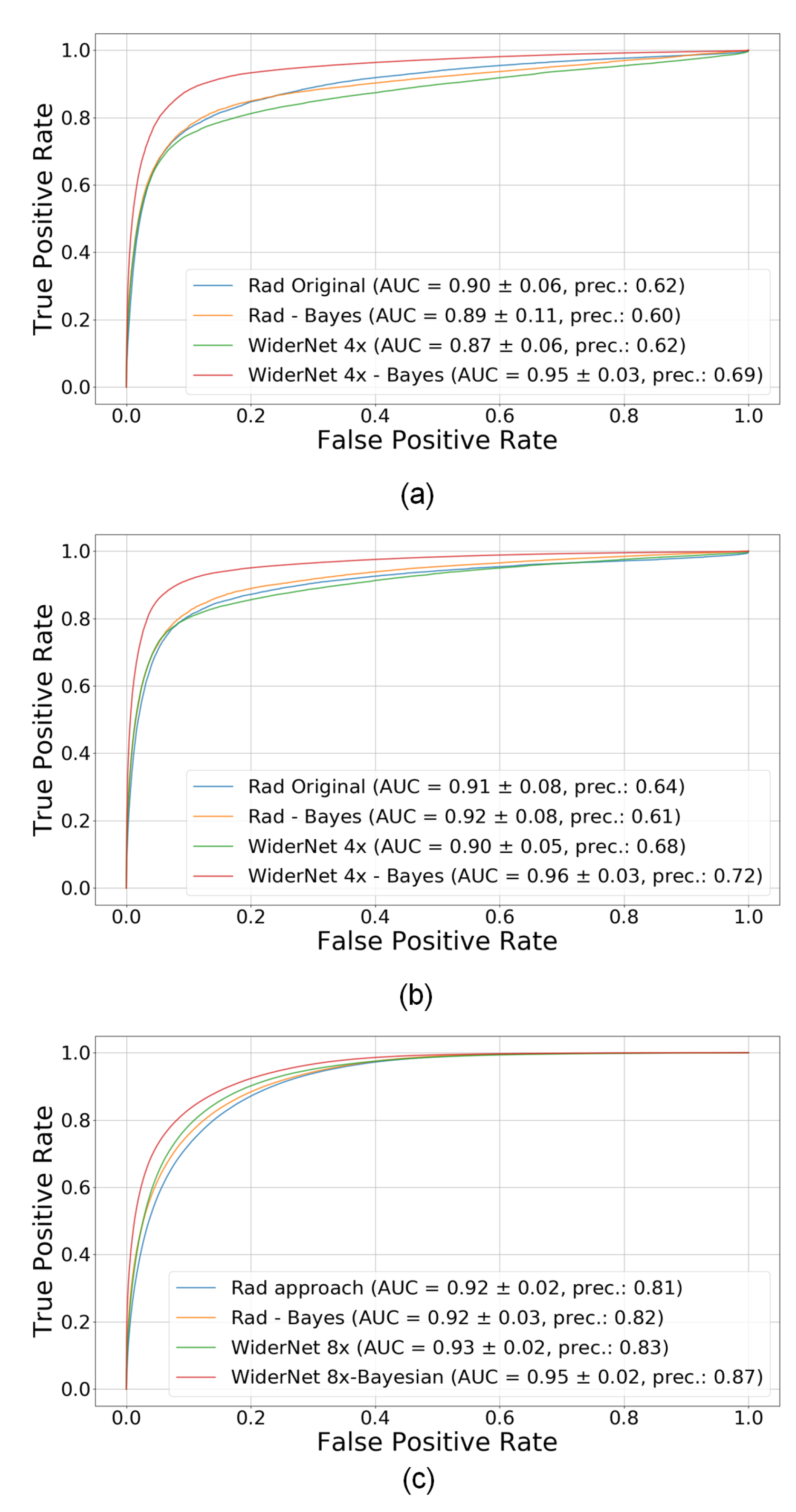
ROC curves for each dataset for Rad’s model and WiderNet 8×, FCN 128 (i.e., with 128 neurons in their fully connected layer). (a) EDAQA dataset, study 1, (b) EDAQA dataset, study 2, (c) ESDB dataset. The Bayesian model with the higher capacity performs best in all datasets. Best viewed in color.
Figure 4.
ROC curves for each dataset for Rad’s model and WiderNet 8×, FCN 128 (i.e., with 128 neurons in their fully connected layer). (a) EDAQA dataset, study 1, (b) EDAQA dataset, study 2, (c) ESDB dataset. The Bayesian model with the higher capacity performs best in all datasets. Best viewed in color.

Figure 5.
Area from the diagonal of reliability plots with and without transfer learning (TF). TF prevents this error metric from increasing as the model capacity increases. Best in color.
Figure 5.
Area from the diagonal of reliability plots with and without transfer learning (TF). TF prevents this error metric from increasing as the model capacity increases. Best in color.

Figure 6.
Distribution of correct and incorrect predictions for WiderNet 8×, FCN-128 on the ESDB dataset. Please note that that the entropy has different distributions for the (a) correct vs. (b) incorrect predictions. This indicate that it is a good feature for quantifying the uncertainty (i.e., higher entropy means higher likelihood of having an incorrect prediction). Best in color.

Figure 7.
F1-Score vs. Precision plot using uncertainty selection for ESDB dataset. The performance is obtained by setting the predictions of the model to a negative detection if their uncertainty follows below the specified calibrated probability or entropy thresholds. The original model is WiderNet 8×, FCN 128 with Bayesian approach and no selection. Please note that the curve produced by the cal. prob. is better than the entropy curve. Furthermore, a threshold of 0.65 on the cal. prob. yields almost no drop in F1-score but and 7% increase in precision. Best viewed in color.

Figure 8.
Precision vs. Recall plot for uncertainty selection on ESDB dataset. The original model is WiderNet 8×, FCN 128 with Bayesian approach and no selection. Please note that a threshold of 0.65 on the cal. prob. yields about an equal percentage of increase in precision and decrease in recall. Best in color.

Figure 9.
AUC score vs. Percentage of samples kept unchanged for uncertainty selection on ESDB dataset. Each curve shows the corresponding threshold values used for the data points. The original model is WiderNet 8×, FCN 128 with Bayesian approach. Best viewed in color.
Figure 9.
AUC score vs. Percentage of samples kept unchanged for uncertainty selection on ESDB dataset. Each curve shows the corresponding threshold values used for the data points. The original model is WiderNet 8×, FCN 128 with Bayesian approach. Best viewed in color.

Figure 10.
Comparison for ESDB dataset considering a Utopian case where ground truth values are also removed if the associated calibrated probability is smaller than the selection threshold. Best viewed in color.
Figure 10.
Comparison for ESDB dataset considering a Utopian case where ground truth values are also removed if the associated calibrated probability is smaller than the selection threshold. Best viewed in color.


Table 1.
Datasets.
| Name | Subject | Session | Total Length | Occurrences | Behavior Duration | Sensors |
|---|---|---|---|---|---|---|
| ESDB | 1 | 14 | 11.74 h | 526 | 7 h (59.7%) | Acc, Gyro |
| EDAQA | 6 | 25 | 10.63 h | 792 | 2 h (20.3%) | Acc |
† Limb: Right upper arm and wrist; †† Limb: Right/Left wrists, torso.
Table 2.
BNN equation summary.
| Equation | Title | |
|---|---|---|
| (1) | Representation of a DNN with L layers | |
| (2) | Standard loss function for a DL model | |
| (3) | Model predictive probability | |
| (4) | Loss function of Gaussian Process | |
| (5) | Monte Carlo approximation of (4) | |
| (6) | Regression loss obtained from (5) | |
| (14) | Classification loss obtained from (5) | |
| (10) | Model predictive variance | |
| (11) | Model predictive entropy | |
| + | (12) | Mutual information |
Table 3.
Summary of averaged performance for each dataset.
| Study 1 | Study 2 | ESDB | ||
|---|---|---|---|---|
| Rad Original | AUC: | 0.896 | 0.906 | 0.916 |
| F1: | 0.549 | 0.580 | 0.841 | |
| Precision | 0.620 | 0.680 | 0.810 | |
| Rad Bayes | AUC: | 0.891 | 0.920 | 0.925 |
| F1: | 0.502 | 0.530 | 0.852 | |
| Precision | 0.690 | 0.720 | 0.820 | |
| WiderNet 2× | AUC: | 0.895 | 0.921 | 0.929 |
| F1: | 0.584 | 0.636 | 0.855 | |
| Precision | 0.640 | 0.670 | 0.830 | |
| WiderNet 2× | AUC: | 0.941 | 0.958 | 0.943 |
| Bayes | F1: | 0.612 | 0.679 | 0.867 |
| Precision | 0.660 | 0.710 | 0.860 | |
| WiderNet 4× | AUC: | 0.885 | 0.920 | 0.930 |
| F1: | 0.587 | 0.653 | 0.857 | |
| Precision | 0.640 | 0.670 | 0.830 | |
| WiderNet 4× | AUC: | 0.948 | 0.961 | 0.946 |
| Bayes | F1: | 0.645 | 0.695 | 0.870 |
| Precision | 0.680 | 0.710 | 0.860 | |
| WiderNet 8× | AUC: | 0.869 | 0.903 | 0.929 |
| F1: | 0.554 | 0.602 | 0.856 | |
| Precision | 0.620 | 0.680 | 0.830 | |
| WiderNet 8× | AUC: | 0.945 | 0.960 | 0.947 |
| Bayes | F1: | 0.655 | 0.703 | 0.870 |
| Precision | 0.690 | 0.720 | 0.870 | |
| WiderNet 16× | AUC: | 0.838 | 0.892 | 0.926 |
| F1: | 0.529 | 0.570 | 0.852 | |
| Precision | 0.560 | 0.670 | 0.830 | |
| WiderNet 16× | AUC: | 0.943 | 0.954 | 0.945 |
| Bayes | F1: | 0.654 | 0.700 | 0.866 |
| Precision | 0.700 | 0.730 | 0.870 |
Publisher’s Note: MDPI stays neutral with regard to jurisdictional claims in published maps and institutional affiliations. |
© 2022 by the authors. Licensee MDPI, Basel, Switzerland. This article is an open access article distributed under the terms and conditions of the Creative Commons Attribution (CC BY) license (https://creativecommons.org/licenses/by/4.0/).
Share and Cite
MDPI and ACS Style
da Silva, R.L.; Zhong, B.; Chen, Y.; Lobaton, E. Improving Performance and Quantifying Uncertainty of Body-Rocking Detection Using Bayesian Neural Networks. Information 2022, 13, 338. https://0-doi-org.brum.beds.ac.uk/10.3390/info13070338
AMA Style
da Silva RL, Zhong B, Chen Y, Lobaton E. Improving Performance and Quantifying Uncertainty of Body-Rocking Detection Using Bayesian Neural Networks. Information. 2022; 13(7):338. https://0-doi-org.brum.beds.ac.uk/10.3390/info13070338
Chicago/Turabian Styleda Silva, Rafael Luiz, Boxuan Zhong, Yuhan Chen, and Edgar Lobaton. 2022. "Improving Performance and Quantifying Uncertainty of Body-Rocking Detection Using Bayesian Neural Networks" Information 13, no. 7: 338. https://0-doi-org.brum.beds.ac.uk/10.3390/info13070338
Note that from the first issue of 2016, this journal uses article numbers instead of page numbers. See further details here.