Adaptive Savitzky–Golay Filters for Analysis of Copy Number Variation Peaks from Whole-Exome Sequencing Data

Abstract

Copy number variation (CNV) is a form of structural variation in the human genome that provides medical insight into complex human diseases; while whole-genome sequencing is becoming more affordable, whole-exome sequencing (WES) remains an important tool in clinical diagnostics. Because of its discontinuous nature and unique characteristics of sparse target-enrichment-based WES data, the analysis and detection of CNV peaks remain difficult tasks. The Savitzky–Golay (SG) smoothing is well known as a fast and efficient smoothing method. However, no study has documented the use of this technique for CNV peak detection. It is well known that the effectiveness of the classical SG filter depends on the proper selection of the window length and polynomial degree, which should correspond with the scale of the peak because, in the case of peaks with a high rate of change, the effectiveness of the filter could be restricted. Based on the Savitzky–Golay algorithm, this paper introduces a novel adaptive method to smooth irregular peak distributions. The proposed method ensures high-precision noise reduction by dynamically modifying the results of the prior smoothing to automatically adjust parameters. Our method offers an additional feature extraction technique based on density and Euclidean distance. In comparison to classical Savitzky–Golay filtering and other peer filtering methods, the performance evaluation demonstrates that adaptive Savitzky–Golay filtering performs better. According to experimental results, our method effectively detects CNV peaks across all genomic segments for both short and long tags, with minimal peak height fidelity values (i.e., low estimation bias). As a result, we clearly demonstrate how well the adaptive Savitzky–Golay filtering method works and how its use in the detection of CNV peaks can complement the existing techniques used in CNV peak analysis.

1. Introduction

Copy number variation (CNV), which includes DNA segments longer than one kilobase pair being amplified or lost, is a significant class of DNA structural variants [1]. The mutation rate of CNV loci is significantly higher than that of SNPs across the entire genome, making CNV an important pathogenic factor causing human complex diseases [2]. The three main technology types that can generate data sets for the detection of CNVs are array comparative genomic hybridization (aCGH), SNP array, and next-generation sequencing (NGS). NGS can perform target capture sequencing such as whole-exome sequencing (WES). This is one of the techniques widely used to extract genomic information from a specific exome region of interest using customized probes in clinical diagnosis [3]. This technique is cost-effective and provides much higher coverage than whole-genome sequencing (WGS) for the identification of rare variants and can provide exceptional prospects for researchers and patients [4]. However, some of the limitations of this technique include the following: first the information is not continuous (i.e., not every position is covered such as intergenic regions, large introns, promoters they are ≈99% of the genome, WES only covers ≈1%); secondly, targeted genomic coordinates (exonic and coding sequences) of different kits equivalent the precise positions of the designed hybridization oligos; third, multiple combinations of oligos exist that could capture the same target region by different kit design based on the position and shape of the coverage profile of sequence data resulting from these kits and only loosely corresponds with the genome coordinates of targeted regions [4,5]. Lastly, the exact position of the hybridization oligos is unknown, hence they could only be inferred from the experimental NGS sequence data [6]. Thus, due to the unique features of NGS, the CNV detection methods involving targeted NGS data could be divided into four categories, notably, split-read-, de novo assembly-, pair-end-mapping- and read depth (RD)-based approaches [7,8]. The read depth-based approach is more robust in detecting CNVs of any sizes other among three categories. This method’s main tenet is to detect CNVs based on the variation of read depths a cross the genome to be investigated [9]. Currently, there are several techniques for detecting CNVs using RD values; however, these techniques frequently have unique characteristics and limitations [10,11]. The analysis of CNVs peaks with small amplitudes is still challenging due to factors such limited coverage depth and GC content bias, despite the techniques’ considerably strong performance [12]. Therefore, an appropriate filtering method is necessary to filter the CNVs peaks. Several filtering methods have been proposing for peak processing, including spline smoothing [13], Stein’s unbiased risk estimate (SURE) [14], Fourier transform [15], Gaussian Kernel filtering [16], Epanechnikov Kernel [17], Lowess [18], Savitzky–Golay [19] and discrete wavelet transform [20]. Some of those filtering methods experience computational challenges when handling highly corrupted signals. Savitzky–Golay has been widely used in biomedical electrocardiogram (ECG) signal processing due to its ability to achieve high signal-to-noise ratio and retains the original shape of the signal [21]. Though this method has been widely used for signal processing, no study has reported its application in CNV peak detection and analysis. Currently, some of popular methods for detecting and analyzing CNVs include, but is not limited to, CNVkit [22], Control-FREEC [23], iCopyDAV [24], PEcnv [25] and CNV_IFTV [26]. Each of these methods has its own characteristics and advantages. For example, CNVkit uses both the targeted reads and the nonspecifically captured off-target reads to infer copy number evenly across the genome to identify copy number changes based on we evaluation of three sources of bias in the sequencing read depth: GC content, target footprint size and spacing, and repetitive sequences [27]. Control-FREEC most effectively utlizes GC-content to normalize the read count profile so as to find out CNV regions, and iCopyDAV chooses an appropriate bin size and uses thresholds for RD values to declare CNVs. Although much effectiveness has been achieved by these methods, limited coverage depth and GC-content bias still pose a big challenge to the detection of CNVs with small amplitudes. Therefore, it would be necessary and meaningful to seek for new methods that can grasp the essential characteristics of sequencing data associated with CNVs. In this study, we proposed an adaptive Savitzky–Golay filtering method for the detection and analysis of CNV peaks obtained from WES data. The motivation for the underlying axiom of our novel approach is as follows: it uses the existing concepts of local polynomial regression (LPR) and least squares criterion (LSC) to model the peak distribution function. It provides a generic framework for an adaptive Savitzky–Golay that automatically chooses the polynomial order and window length based on the peak distribution, allowing for accurate smoothing of peaks with high rates of change as well. It consider peak positions in each segment by calculating local density and minimum distance in order to extract two related features from the CNV peaks profile. Finally, using a multivariate Gaussian distribution, It calculate the associated p-value for the CNV peak from the feature values. We conducted numerous simulation studies to evaluate and compare our approach to peer methods. The experimental findings show the effectiveness of the method.

The rest of this article is organized as follows: In Section 2, we provide a model equation of peak distribution function, then we present a mathematical formulation of the classical Savitzky–Golay filter and adaptive Savitzky–Golay filter with respect to CNVs peak function; next, we describe a new formulation of feature extraction for CNV peak detection and analysis. In Section 3, we present the results of model performance evaluation and its application to real WES data generated for germline mutation analysis. In Section 4, we summarize the discussion of the proposed method’s and genetic implication with respect to CNV peak detection and analysis. In Section 5, we conclude and outline our plans for future work.

2. Materials and Methods

2.1. Peak Distribution Function

Generally, peak distribution tends to be asymmetrical in nature; therefore, it is important to develop a function that is applied to a wide class of the peak distribution. Let us consider the existing concept of local polynomial regression (LPR) [28] and the least squares criterion (LSC) [29]; thus, the peak distribution function is given by equation

$$f\left(S_i\right)=f_0\left(S_i\right)+w\left(S_i\right),i=1,\dots n,$$

(1)

where $f\left(S_i\right)$ is the main peak, $f_0\left(S_i\right)$ is the noisy peak and $w\left(S_i\right)$ is identically distributed $\left(iid\right)$ additive white Gaussian noise of mean zero and variance ${\sigma }^2$, S is the segment. To keep things simple, we will represent a peak $f_0$ at $i^{th}$ segment by $f_i\triangleq f\left(S_i\right)$ and w at i^th segment by $w_i\triangleq w\left(S_i\right)$.

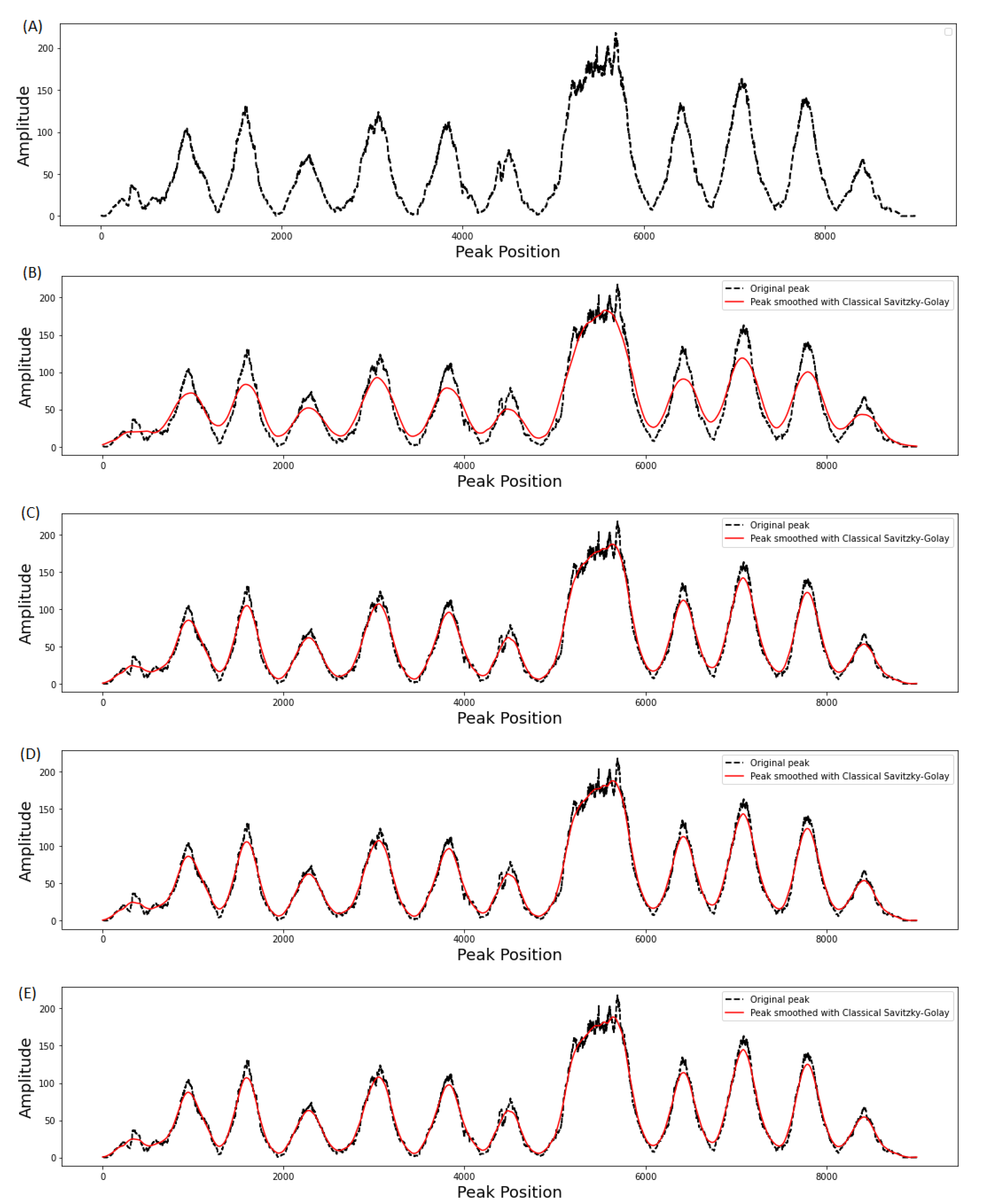
2.2. Classical Savitizky–Golay Filtering

In this subsection, we provide a summary of the mathematical formulation of classical Savitizky–Golay filtering, based on the work of [30]. We first perform the polynomial fit to obtain the filtered output value by computing the polynomial coefficients at the central index of the approximation window. We then consider a symmetrical window length $M=2m+1$, $i=-m,\dots ,\lambda ,\dots ,m$ with data point x at a reconstruction point $\lambda$ represents the index of the middle point at 0. Thus, the $k^{th}$ order of the polynomial P is calculated by

$$P=f_0+f_1\left(x-x_{\lambda }\right)+f_2{\left(x-x_{\lambda }\right)}^2+\cdots +f_k{\left(x-x_{\lambda }\right)}^k,$$

(2)

The aim is to fit a polynomial of order $P={\displaystyle \sum _{k=0}^N}{f}_k{\left(S_i\right)}^k$ in a least square manner by minimizing the cost function using equation

$${\epsilon }_N=\stackrel{M}{\sum _{i=-M}}{\left(P-x_{\lambda }\right)}^2=\underset{i=-M}{\sum ^M}{\left(\stackrel{N}{\sum _{k=0}}{f}_k{\left(S_i\right)}^k-x_{\lambda }\right)}^2,$$

(3)

To obtain data point at the central index 0 with zeroth polynomial coefficient as $y_0=P_0=f_0$, we calculate an optimal polynomial coefficient by differentiating ${\epsilon }_N$ in Equation (2) with respect to $N+1$ unknown coefficients and setting the derivatives to zero to obtain the following sets of equations

$$\frac{\partial {\epsilon }_N}{\partial f_i}=\stackrel{M}{\sum _{i=-M}}2{\left(S\right)}^i\left(\stackrel{N}{\sum _{k=0}}{f}_k{\left(S\right)}^k-x\left[x_{\lambda }\right]\right)=0,$$

(4)

so, by interchanging the order of the summation, the set of $N+1$ equations in $N+1$ unknown is given by

$$\stackrel{N}{\sum _{k=0}}\left(\stackrel{M}{\sum _{i=-M}}{\left(S\right)}^{i+k}\right)f_k=\stackrel{M}{\sum _{i=-M}}{\left(S\right)}^i\left[x_{\lambda }\right],$$

(5)

Therefore, we can write Equation (5) in matrix form by defining the design matrix $\mathbf{A}=\left\{{\alpha }_{\lambda ,i}\right\}$ i.e., $\left(2M+1\right)\times \left(N+1\right)$ for the polynomial approximation. The transpose of $\mathbf{A}$ as ${\mathbf{A}}^T=\left\{{\alpha }_{i,\lambda }\right\}$ and the product matrix $\mathbf{B}={\mathbf{A}}^T\mathbf{A}$ as $\left(N+1\right)\times \left(N+1\right)$ symmetric matrix. Then, polynomial coefficient vector is given by $\mathbf{f}={[f_0,f_1,\dots ,f_k]}^T$ and input samples vector by $\mathbf{x}={[x_{\lambda -m},\dots ,x_{\lambda -m},x_{\lambda },x_{\lambda +m},\dots ,x_{\lambda +m}]}^T$ where, $x_{\lambda }=x=0$. Hence the desired matrix form of normal equation is expressed as $\mathbf{Bf}={\mathbf{A}}^T\mathbf{Af}={\mathbf{A}}^{T}x$ and solution for the polynomial coefficient is expressed as $f={\left({\mathbf{A}}^T\mathbf{A}\right)}^{-1}{\mathbf{A}}^{T}x=\mathbf{Hx}$, where $\mathbf{H}$ matrix is independent of the input samples (it depends only on M and N). Therefore, the output sample can be computed by the convolution equation

$$f_{\lambda -m}=\stackrel{M}{\sum _{m=-M}}{h}_m{x}_{\lambda -m}=\stackrel{\lambda +M}{\sum _{m=\lambda -M}}{h}_{\lambda -m}{x}_{\lambda },$$

(6)

where $h_{-m}=h_{0,m}=\tilde{p}\left(n\right)-M\le m\le M$, and $h_{i,n}$ is the element of the $\left(N+1\right)\times \left(2M+1\right)$ matrix $\mathbf{H}$ and $h_{0,m}$ is the element of the 0^th row.

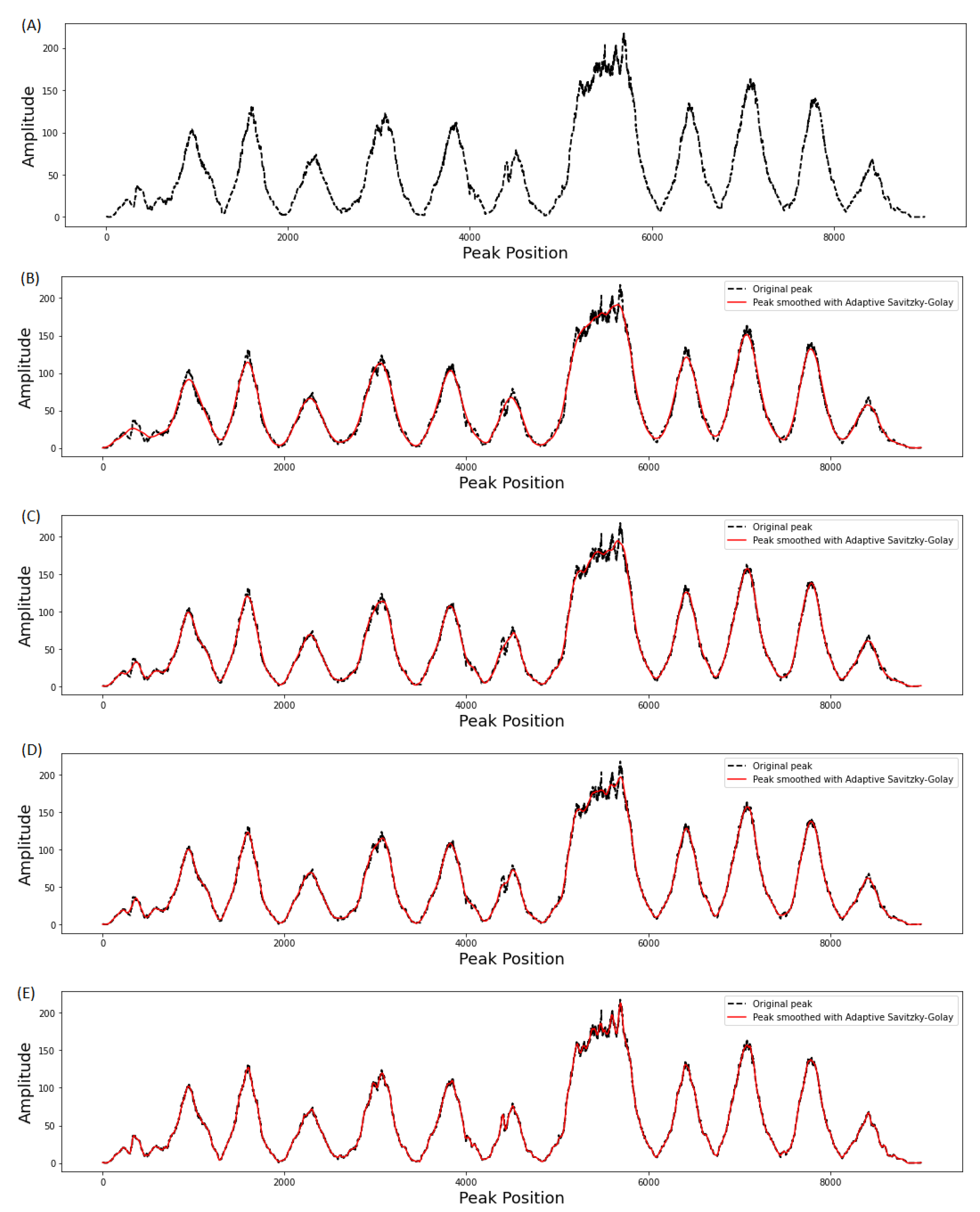
2.3. Adaptive Savitizky–Golay Filtering

In this subsection, we describe our proposed Adaptive Savitizky–Golay filter as an improvement of the existing classical Savitizky–Golay filter. Classical Savitizky–Golay filtering is often used to separate the noisy peak in a given peak distribution pattern with assumption that only the corrupted peaks are available and the aim to identify those peaks. First we consider window length $\left(M\right)$ and degree of the polynomial $\left(k\right)$ to be arbitrary. Thus, we express the coordinates of the local minimum and maximum points of the initial smoothing in the following order

$$C=\left(\begin{array}{cccc}{x}_1& x_2& \cdots & x_u\\ y_1& y_2& \cdots & y_u\end{array}\right),$$

(7)

We introduce d to be the distance vector containing the number of samples between two neighboring points of local minima and maxima to be

$$d=\left({\delta }_1{\delta }_2\cdots {\delta }_{u-1}\right),$$

(8)

Let $S=[s_1,\dots ,s_1]$ be the number of peak with same amplitude in a given segment of peak distribution. Thus, variance neighboring peak points between the $\delta$ local extrema are determined step-wise by equation

$${\sigma }_{\left(d\right)}=\frac{1}{\left(u-1\right){\displaystyle \sum _{i=1}^{u-1}}{\delta }_i^2-{\overline{\delta }}^2},$$

(9)

The actual variance calculated above based on the previous values $>>{\epsilon }_1$. This forms the first segment of the next part; however, the window must match the spread peak distribution while the polynomial degree must vary depending on the frame-size and peak distribution. Thus, each segment consisting of peaks with similar peak height (amplitude) we applied window length $\left(M\right)$ and polynomial degree $\left(k\right)$ based on fuzzy relation given by equation

$$F\left(d_{max}\gg {\overline{d}}_S\right)=\frac{1}{1+e^{-\left(d_{max}-{\overline{d}}_S\right)}}\in \left[0,1\right],$$

(10)

where ${\overline{d}}_S$ is the average length of the segments in the current S parts of the peak distribution, while ${\delta }_{max}=max\left(d\right)$ is the observed peak. If $f\left(d_{max},{\overline{d}}_S\right)=1$ is the peak with highest amplitude in that particular segment. Hence, once we have the coordinates of the local minimum and maximum peak points and the vector d, we assign the k and M values to each S segment using some fuzzy rules, then we apply multi-round linear approximation method according previous work [31] for parameter update. The purpose is to identify the imprecision or inflexion points after the first adaptive Savitizky–Golay smoothing; thus, correction processes enable the introduction of new cutting points for the next adaptive smoothing.

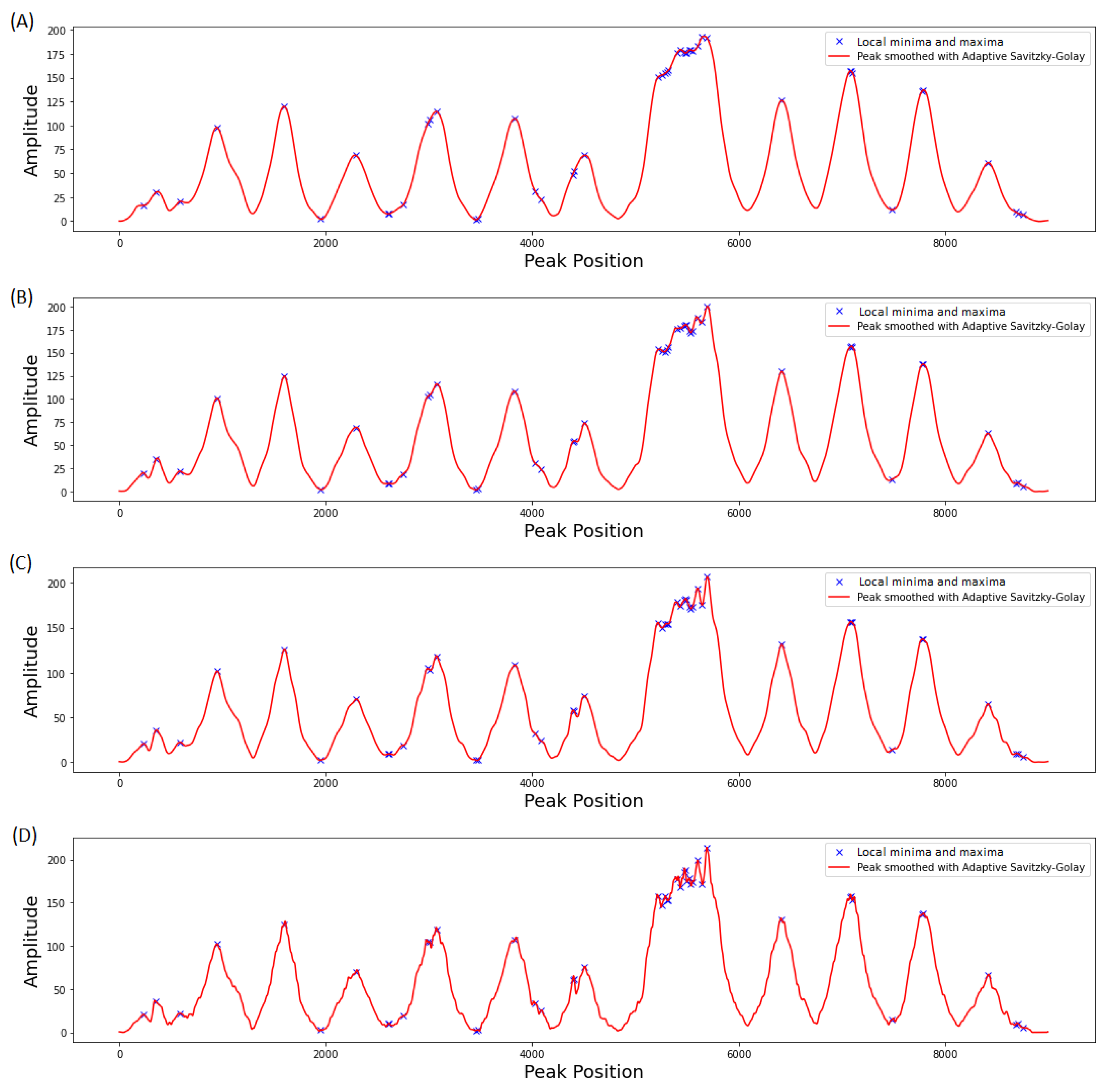
2.4. Feature Extraction

To extract feature statistics from the filtered peak we denote peak segment by S; thus, $S=\left\{s_1,s_2,s_3,\dots ,s_n\right\}$, where n denotes the total number of segments obtained. Hence, based on set of S, we extract feature statistic for each segment of CNVs by calculating the local density $\left(\rho \right)$ and minimum distance $\left(\delta \right)$ to obtain the corresponding values of the neighboring peaks in each segments. With the consideration of that regions with changed copy numbers are inherently different from those of normal copy numbers and only account for a small part of the whole genome, we transfer the problem of detecting CNVs to the issue of identifying outliers from the set of segments with features of $\left(\rho \right)$ and $\left(\delta \right)$. Accordingly, each segment can be regarded as an object or a point in the two dimensional space of $\left(\rho \right)$ and $\left(\delta \right)$. In the following text, we provide a detailed description to these two features and the calculation approach. Before we describe the two features $\left(\rho \right)$ and $\left(\delta \right)$, we introduce the Euclidean distance between two segment $s_i$ and $s_j$. Given two segment $s_i$ and $s_j$ with equal length l, we can obtain an Euclidean distance matrix $M_{l\times l}$ to measure the distance between each element $\left(d_{ij}\right)$ using the Euclidean distance formula

$$d_{ij}=\sqrt{{\left(s_i\left({\rho }_i\right)-s_j\left({\rho }_j\right)\right)}^2+{\left(s_i\left({\delta }_i\right)-s_j\left({\delta }_j\right)\right)}^2},$$

(11)

where ${\rho }_i$ and ${\delta }_i$ are the feature values of a given genomic segment $s_i$ and $s_j$, same apply to ${\rho }_j$ and ${\delta }_j$. Again, using distance matrix $M_{l\times l}$, we calculate the number peaks adjacent to the peaks in segment $s_i$ by equation

$${\rho }_i=\underset{j\ne i}{\sum ^n}\chi \left(d_{ij}-\gamma \right),$$

(12)

where $\chi \left(x\right)=1$ if $x<0$, otherwise $\chi \left(x\right)=0$, ${\rho }_i$ is the local density, $\gamma$ is adjustable distance threshold. Next, we calculate the minimum distance between the peaks with higher density values in segment $s_i$ to rest of peaks by equation

$${\delta }_i=\underset{j:{\rho }_i<{\rho }_j}{min}\left(d_{ij}\right)$$

(13)

where ${\delta }_i$ is the minimum distance defined as the minimum value among the distances between the peaks in segment $s_i$ and those peaks with higher density than segment $s_i$. Similarly, we can calculate the maximum distance between the peak with highest density in segment S by equation

$${\delta }_i=\underset{j}{max}\left(d_{ij}\right)\mathrm{if}{\rho }_i\ge \underset{j\ne i}{{\rho }_j},$$

(14)

where ${\delta }_i$ is the maximum distance defined as the maximum distance between the peak in segment $s_i$ and the rest of peaks in the set S. Lastly, if we assume the smoothed peaks have normal distribution, using multivariate Gaussian distribution function [32], we can extract the feature statistic for each segment using equation

$$f(x,\mu ,K)=\frac{1}{\left(2\pi \right){\left|K\right|}^{\frac{1}{2}}}exp\left(-\frac{1}{2}{\left(x-\mu \right)}^{T}K\left(x-\mu \right)\right),$$

(15)

where $\mathbf{\mu }$ is the two-dimensional vector corresponding to the mean values of local density and minimum distance, i.e., $\mu =[\rho ,\delta ]$, and K is the covariance matrix of the two features.

3. Results

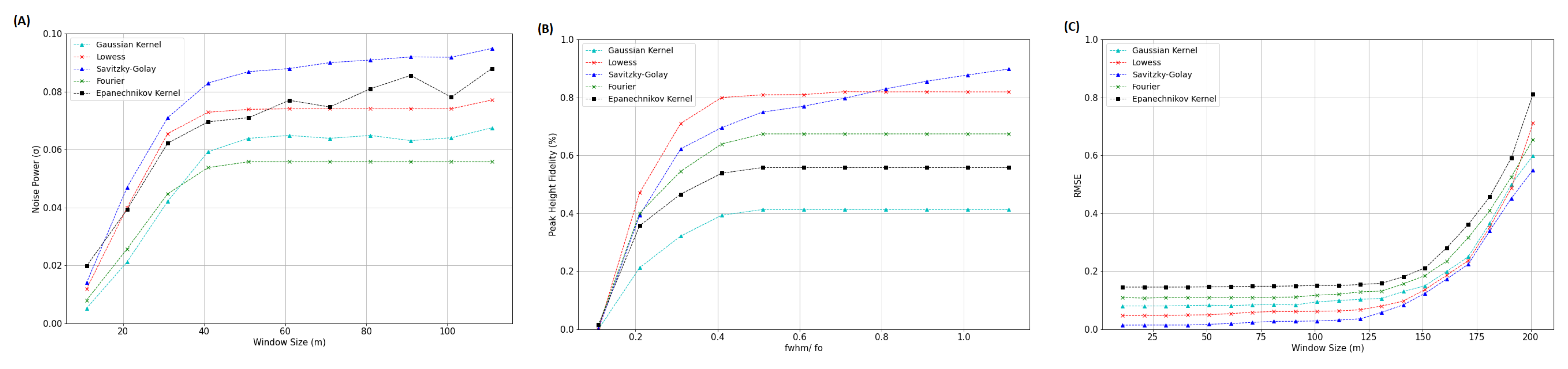
3.1. Effect of Window Length on Smoothing Performance

We evaluate the smoothing performance of both classical Savitzky–Golay filter Section 2.2 and adaptive Savitzky–Golay filter Section 2.3 using sharpening concept, a technique based on standard window function convolution [33]. First we consider the corrupted peak $f\left(S_i\right)$ by a noise with $\sigma =1$. We then show the effect of standard window function convolution on overlapping noisy peaks filtered by classical Savitzky–Golay and adaptive Savitzky–Golay at different polynomial order k and window lengths as shown in Figure 1 and Figure 2, respectively. From the results we observe that at short window length ($m_1=53$), classical Savitzky–Golay has a low bias and high variance in compared larger window length (i.e., $m_3=153$, $m_2=201$ and $m_1=253$). On the other hand, adaptive Savitzky–Golay shows low bias and high variance in larger window length (see red solid line in Figure 1). According the analysis, for classical Savitzky–Golay filter an increase in window length leads to an increase in smoothing bias and decrease in variance. However, adaptive Savitzky–Golay an increase in window length have minimal or no effect on smoothing bias and variance (see red solid line in Figure 2); this is because the method automatically selects the polynomial order ($k$) and window length M based on the peak distribution, allowing peaks with a high rate of change to be smoothed accurately.

According Figure 3, the outcome of the subsequent adaptive SG-smoothing. It is clear that the soft cambers are tracked and the shape of the peak distribution is preserved with proper noise component removal. In the case of an asymmetric peak distribution, this iterative method of smoothing and correction performs well. To accomplish this, we first conduct a quick and easy calculation of the coefficients, after which we conduct a high-speed resampling of the peaks to align with the smaller running window. Next, we use straightforward nearest neighbor interpolation to replace the missing values. Furthermore, we investigated the relationship of window function convolution and stopband attenuation for two overlapping noisy peaks based on the calculation of the near-boundary values to find local minima and maxima peaks (i.e., we simply use the polynomial fit over the $2m+1$ neighborhood closest to the boundary). We assume that the noisy peak and the filtered peaks are at or near the boundary with each other and calculate the peak height fidelity based on local minima and maxima values.

The results of identified local minima and maxima values at different window length by the proposed adaptive Savitzky–Golay filterig are shown in Figure 4. The blue stars are the detected local minima and maxima peak values. From these results, we observe that adaptive Savitzky–Golay filter would reduce the peaks to ≈5% of their original height since the algorithm uses a linear approximation of the peaks for precise smoothing. The optimal signal resolution is determined by the local extrema points. The method performs adaptive smoothing and correction iteratively, allowing the shape of fast-varying peaks to be precisely detected.

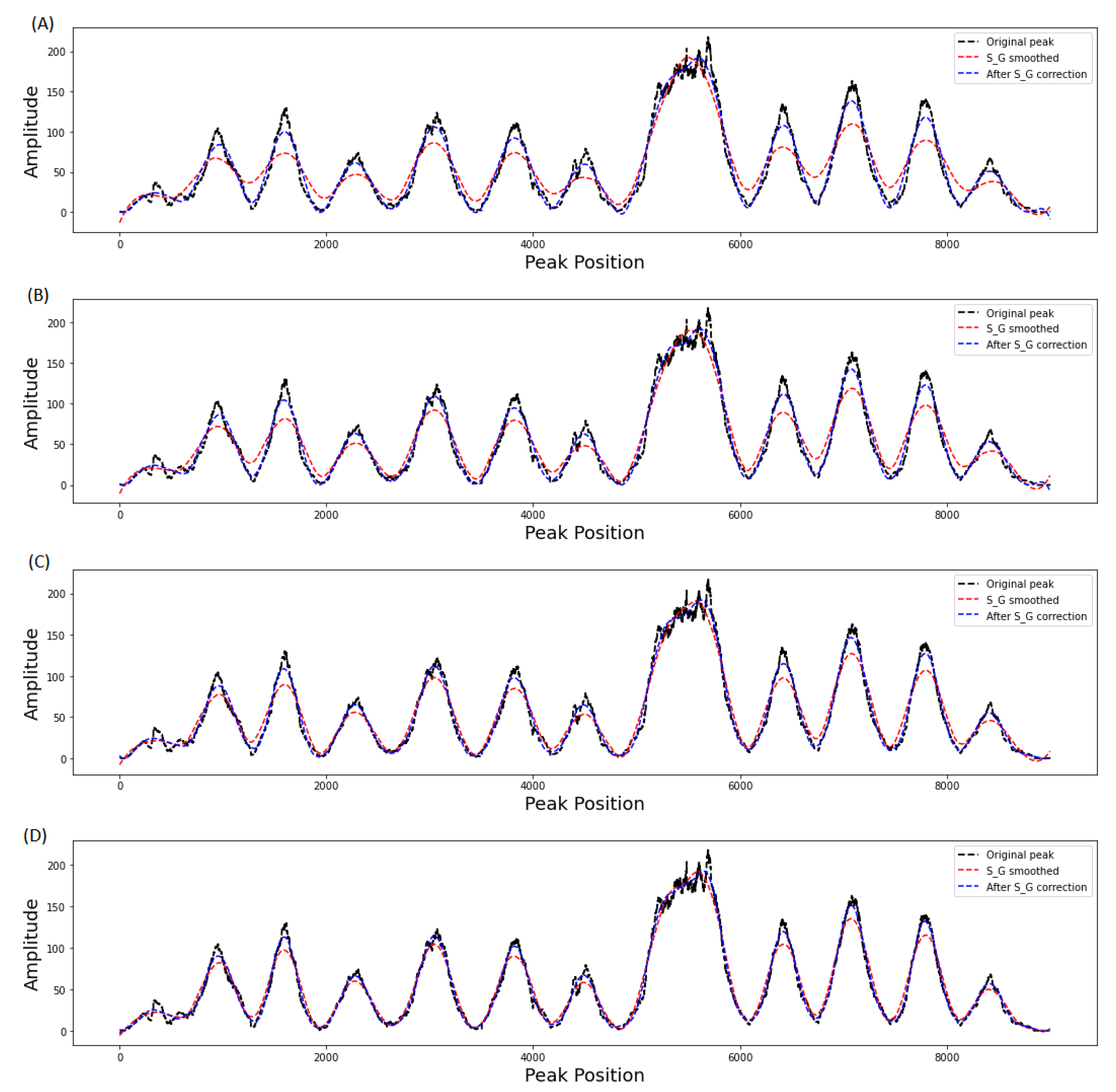
3.2. Evaluation of Filter Order on Smoothing Performance

We evaluate the effect of filter order on smoothing performance by calculation of the minimum mean squared error ($MMSE$) using equation

$$MMSE=r_k{\sigma }^{2k}f{\left(S_i\right)}^{\frac{1}{2k}},$$

(16)

where $r_i$ is noise coefficient, $\sigma$ is the noise power, $f\left(S_i\right)$ is the peak distribution function and k is the filter order. In our simulation, the original peaks were first corrupted the by Gaussian noise with zero mean and two noise power values, i.e., we introduce low noise power ($\sigma =0.05$) and high noise power ($\sigma =1$) at different window to measure minimum MSE. The goal was to check the effect of filter order on estimation error. Simulation results in

Table 1. Effect of filter order on the estimation error.

		${\mathit{k}}_1=2$		${\mathit{k}}_2=3$		${\mathit{k}}_3=4$		${\mathit{k}}_4=5$
Peak	$\mathit{\sigma }$	${\mathit{m}}_1$	$\mathit{MMSE}$	${\mathit{m}}_2$	$\mathit{MMSE}$	${\mathit{m}}_3$	$\mathit{MMSE}$	${\mathit{m}}_4$	$\mathit{MMSE}$
$f\left(S_1\right)$	0.050	11	0.00010	21	0.00006	31	0.00005	41	0.00003
	1.000	33	0.00551	63	0.00326	93	0.00216	123	0.00116
$f\left(S_2\right)$	0.050	11	0.00008	21	0.00007	31	0.00006	41	0.00004
	1.000	33	0.00672	63	0.00421	93	0.00321	123	0.00213
$f\left(S_3\right)$	0.050	11	0.00009	21	0.00008	31	0.00007	41	0.00001
	1.000	33	0.00841	63	0.00554	93	0.00414	123	0.00394

σ, noise power, k filter order, m window length, MMSE minimum mean square error.

show the effect of different filter order on the estimation error. When we perform the adaptive multi-round filter at different polynomial orders, we observed a relatively high MMSE at low filter order ($k_1=2$) and low MMSE at higher filter order. This implies that MMSE is dependent on polynomial order as result leads to computational burden due to least square (LS) fitting. Since the proposed Adaptive Savitzky–Golay filters select the polynomial order automatically, the peaks with a high rate of change are properly smoothed, thus the computational burden associated with higher polynomial order and window length is reduced.

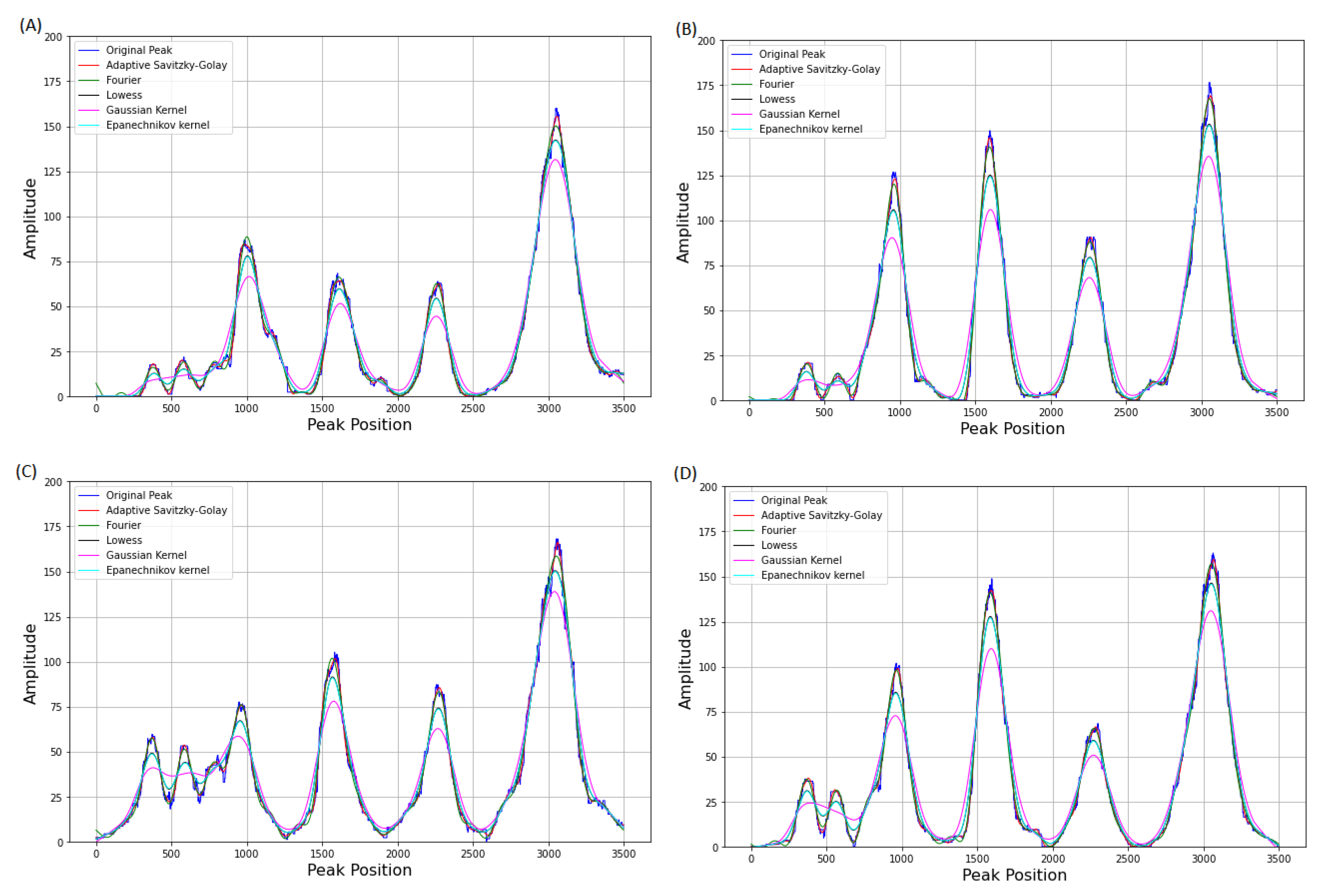
3.3. Comparison of Adaptive Savitzky–Golay Filtering with Peer Methods

We compared the adaptive Savitzky–Golay filters performance with the other peer filtering methods including: Fourier transform [15], Gaussian Kernel filtering [16], Epanechnikov Kernel [17], Lowess [18] smoothing algorithms. In analysis, we use moving average optimal window length approach to compare the smoothing performance. We first corrupted the peaks by adding noise power $\left({\sigma }^2\right)$ to the original peaks. The noise power, i.e., the ratio between the output and input root-mean-square noise, were calculated for white noise. Figure 5A, shows the comparison results of noise suppression. We can observe a non-linear relationship between the noise power and window length, that is an increase in noise power leads to an increase in window length this implies that adaptive Savitzky–Golay have better performance in optimal window length estimation compared to other peer methods. All smoothing methods produce comparable results, with the adaptive Savitzky–Golay filters outperforming the others in terms of noise power. With increasing window length, Fourier smoothing offers slightly less noise suppression than Lowless, Gaussian, and Epanechnikov Kernel. As a result of the more gradual cutoff in the frequency domain, noise suppression of $k_1=2$ filters is slightly weaker than that of higher degrees k filters. In addition, we compared adaptive Savitzky–Golay peak height fidelity to that of other peer filtering methods. In this case, we measure the fwhm peak with 90% peak height fidelity. We measure the white noise gain and define the noise bandwidth as the integral over the kernel’s power spectrum, with the full bandwidth corresponding to the peak function. The gain of the white noise is then proportional to the square root of the bandwidth. Increasing the bandwidth causes less attenuation of a peak with a given full width at half maximum (fwhm); sharper peaks (lower fwhm) require more bandwidth. We can plot the peak height fidelity as a function of the product of the noise bandwidth and the fwhm, which is largely independent of the specific bandwidth or fwhm value.

The merits of the various filters are then shown in Figure 5B. If a specific peak height fidelity (e.g., ≈90% of the original peak height) is required, the curve with the lowest noise bandwidth for white noise—that is, it best suppresses the noise. Convolution with a Gaussian kernel performs the worst, according to the results (except when the peaks are strongly attenuated to less than ≈40% of their original height). The adaptive Savitzky–Golay filters, Lowess, and Fouier filters are nearly equal and best (the difference is less than the line width in), and the Epanechnikov Kernel comes close. The Gaussian kernel filter performs worse than our filters due to poor high-frequency noise attenuation (see Figure 5B). Increasing the bandwidth of Adaptive Savitzky–Golay filtering provides an improve peak height fidelity from ≈63% to ≈90%. In addition, we compare the RMSE of adaptive Savitzky–Golay filters with peer filtering methods. According to Figure 5C, we found that all methods produce similar results; however, adaptive Savitzky–Golay filters recorded a low Root Mean Squared Error (RMSE) due minimal estimation bias (see more additional result in Figure A1, Appendix A).

3.4. Application in CNVs Peak Analysis

Note that our proposed adaptive Savitzky–Golay filtering is a data smoothing and feature extraction tool for CNVs peak profile analysis. Therefore, in our analysis we focus on following aspects: (1) to smooth CNVs and segment the observed RD peak profile, so that adjacent bins with similar peak amplitudes can be merged into the same region and the bins showing a local variation is unmasked; (2) to extract meaningful feature statistic from peak profile data an accurate distinction between mutated and normal genomic regions. (3) to provide a reasonable model for visualising the extracted features to perform a suitable analysis of the features to determine CNVs.

3.4.1. Data Preparation

In this study, experimental WES data generated for germline mutation analysis using the Illumina DNA exome kit were used. For the experimental simulation data, we generated two data sets. We used the coverage depth profile of individual samples (LONG tag) that was based on all reads of the given sample. Furthermore, we generated a validation data set (SHORT) based on the short reads (length $\le 80$ base pairs) of a large cohort of samples. We use “samtools depth” command with the “-a”/output to identify all positions (including zero depth)/and “-b segments.bed” options to query the read depth of interests from our BAM (binary sequence alignment map files).

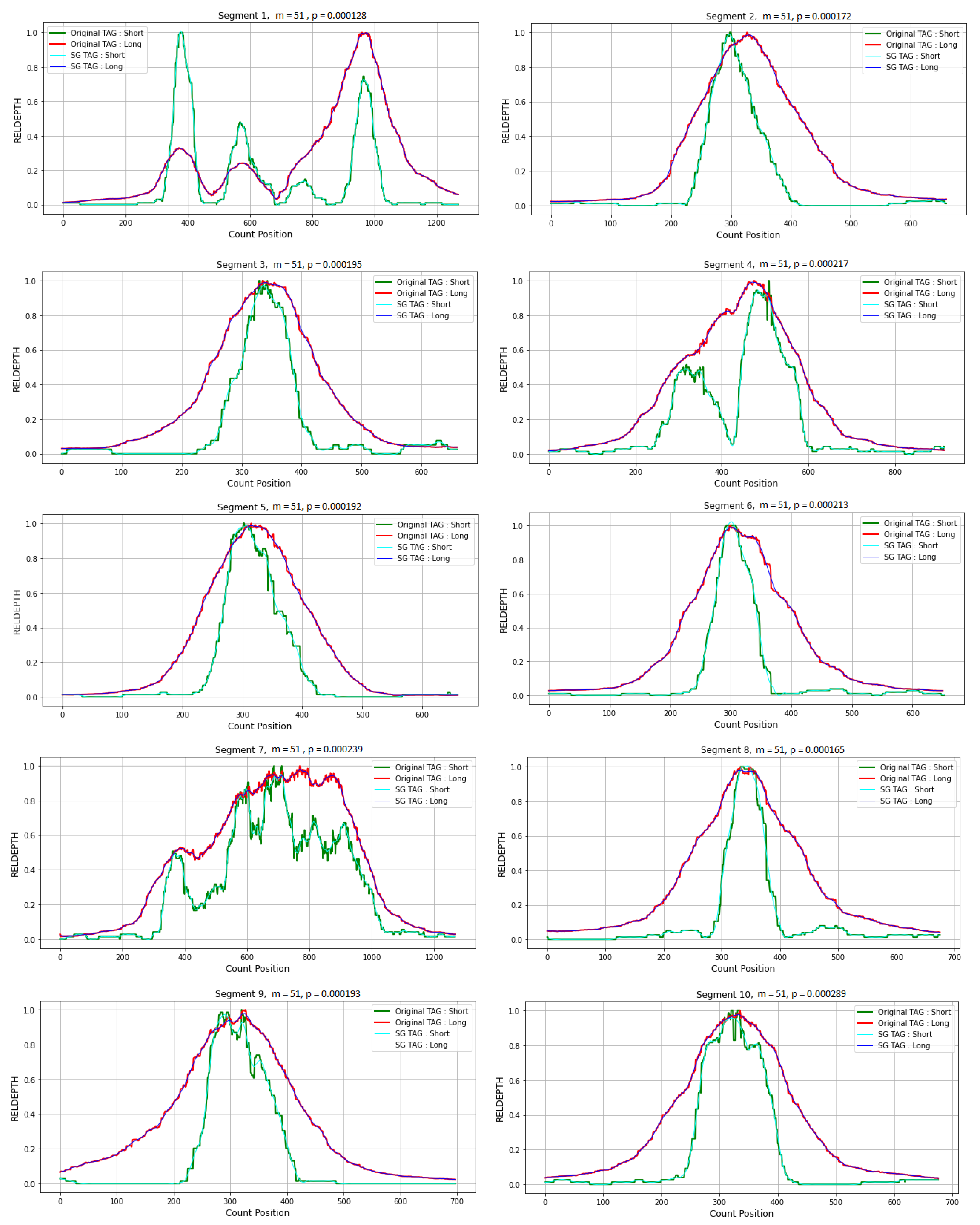
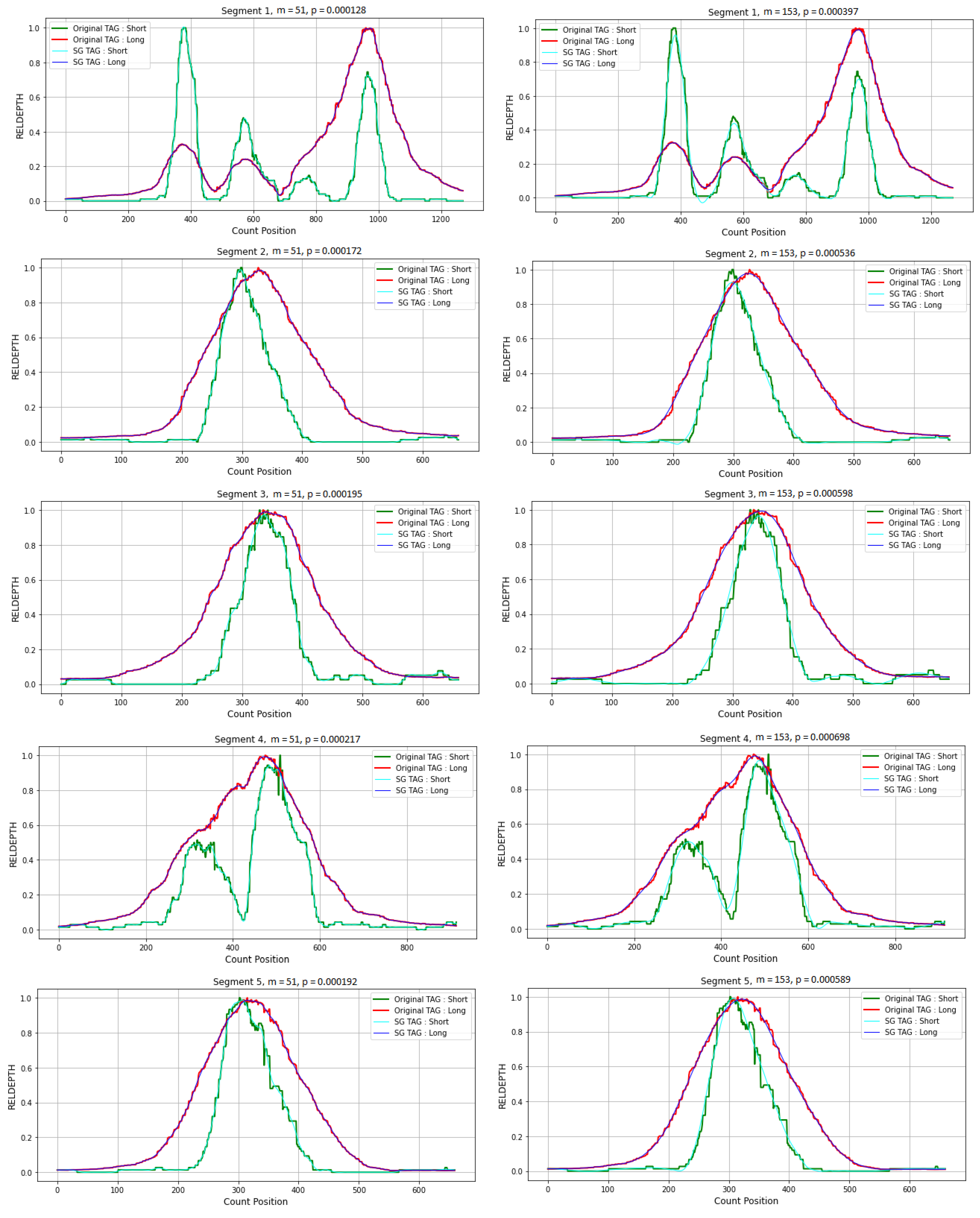
3.4.2. Simulation Studies

Simulation studies are usually regarded as an appropriate and feasible way to assess the performance of existing and newly developed methods [34]. This is because the ground truth CNVs embedded in the simulated data sets could be used for an exact calculation of sensitivity and precision for the methods. CNV peak distribution are often asymmetrically in nature due to variation in depth coverage attributed to the GC bias during the hybridization process. The CNV peak generation often depends on the read depths coverage of the target region and the oligo capture baits within those regions which results into asymmetrical peak distribution. This poses a great challenge smoothing such peaks; thus, it is important to model a peak function that applied to a wide class of the peak distribution patterns obtained from different genomic segments. With a careful consideration of the problems described above, we filtered all CNV peaks for each genomic segments using the proposed adaptive Savitzky–Golay filtering method. For optimal CNV peak filtering, we apply the concept described in Section 2.3. Using Equation (15), the filter order and optimal window length values are automatically computed by adaptive Savitzky–Golay filters. The feature values of CNV peak in each genomic segment were then extracted using Equations (12) and (13). The statistical significance for each peak at given genomic segments was then calculated using Equation (15). According to the results shown in Figure 6, there was significant level of feature extraction for all the genomic segments evaluated for CNV peak (i.e., both long and short tag peaks—also see results in Figure A2 and Figure A3).

4. Discussion

Although several filtering algorithm exists, most of them require the characterization and model parameter tuning for efficient filtering and smoothing of the peaks or signal data [18,35,36,37]. Savitzky–Golay method was originally developed to make discernible the relative widths and heights of spectral lines. The Savitzky–Golay filters are widely used in many fields of data processing, ranging from spectra in analytical chemistry to geosciences and medicine [38]. The SG method was originally developed to make discernible the relative widths and heights of spectral lines. It equally smooths the noise and the signal components, as it leads to bias and a reduction in resolution. For denoising peaks with a large spectral dynamic or with a high rate of change, the classical SG filtering is an unsuitable method [39]. In addition, efficiency depends on the appropriate selection of the polynomial order and the window length, which should match the intrinsic scale of the input peaks. However, the SG-filters provide excellent results while preserving simplicity and speed, but most of the applications require the users to arbitrarily select the polynomial order and size of the sliding window. In general, the SG filters perform well when we apply a low-order polynomial with long window length or low degree with short window and repeated smoothing. It has also been shown that the smoothing effect decreases by applying low-order polynomial on higher frequencies or high-order polynomials on lower frequency parts of the peaks. With this in mind, in this study we introduced an adaptive filtering method based on SG filtering and feature extraction algorithm, which provides good performance independent of the type of noise in the CNV peaks. The proposed technique ensures high-precision noise reduction by iterative multi-round smoothing and correction. In each round, the parameters are dynamically changed due to the results of the previous smoothing. Our approach provides additional support for data compression based on optimal resolution of the peak with linear approximation as well as density and Euclidean-distance-based function for feature extraction as an option to preprocessing CNV peaks. The classical SG-filter depends on the appropriate setting of the window length and the polynomial degree, which should match the scale of the signal, since in the case of signals with high rate of change, the performance of the filter may be limited [19]. Here, simulation results validate the applicability of our approach in the analysis of CNV peak in whole exome sequencing data. Meanwhile, we demonstrated the difference and the robustness of adaptive Savitzky–Golay and its application with other peer filter methods (Fourier [35], Epanechnikov Kernel [36], Gaussian Kernel [37] and Lowess [18]).

Our findings demonstrate the relationship between the adaptive Savitzky–Golay window lengths and filter order (polynomial degree). We discovered that noise suppression is effective when the filter order and window length are set to optimal values. We noted that it is critical to compute the derivative and set an optimal window length before applying the adaptive Savitzky–Golay algorithm to noisy peaks. We have seen, for example, that there is high estimation bias with weak smoothing (e.g., to preserve peak patterns a window length of $m_2=201$ and a filter order of $k_2=3$ is necessary). For strong smoothing, however, the difference between differentiation first and smoothing first grows. As a result of insufficient noise suppression near the boundaries, the “derivative first, then smoothing” is ineffective for strong smoothing. In a broad sense, this shows that adaptive Savitzky–Golay is more effective at noise suppression when the window size is small and the filter order is high (see Figure 1). We also noticed that when comparing different smoothing methods, the trade-off between window size and noise suppression does not always apply. The Gaussian Kernel, on the other hand, has the worst noise suppression at the boundaries in all cases, and its filtered peaks exhibit more estimation bias. As a result, other methods perform better when smoothing near-boundary data in terms of artifacts and noise suppression (see Figure 2). In addition, we found a non-linear relationship between noise power, RMSE, and window size (see Figure 3). Figure 3A shows that Savitzky–Golay has a higher noise power than other peer filtering methods. However, we discovered that adaptive Savitzky–Golayhas has a lower RMSE and performs better. In general, the Fourier, Epanechnikov Kernel, and Gaussian Kernel filters performed noticeably worse in terms of estimation error (RMSE) when compared to the Lowess filtering method, which provided slightly better noise suppression though not effective than adaptive Savitzky–Golay.

Using our proposed peak detection and analysis, we demonstrated the functionality of the adaptive Savitzky–Golay filter for peak smoothing and density-based peak detection methods for the statistical feature extraction of smoothed peaks in each genomic segments. According to the results, we observed that, after filtering WES, we obtained the short- and long-tag CNV peaks in all genomic segments with roughly the same count position when filtering at optimal window size $(m_1=51)$ and filter order $(k_4=51)$. We also noted that adaptive Savitzky–Golay completely suppressed noise at the boundaries of short- and long-tag CNV peaks (see Figure 4). We also discovered that increasing the window size at the fix filter order results in low suppression noise at the boundaries of short- and long-tag CNV peaks, resulting in high peak height fidelity due to under-fitting (high estimation bias). Furthermore, visual inspection reveals that noise suppression at high filter order is nearly as good as convolution with small window length (see Figure A1). Generally, the average read size (220–270 base pair) was larger than the 80bp oligo capture bait size and also that any oligo capture bait could be designed in any position, including partially overlapping positions or gaps less than the peak width we used two approaches to identify the sub peaks corresponding to the designed oligo capture baits in the genomic segments. As the readily available approach, first we used all reads of the samples and for the individual coverage profiles of each samples we tried to infer the position of the sub peaks. In the second approach, we used the fact that average fragment size in a sample is a distribution of randomly broken DNA fragments that includes a small fraction (usually less than 1–2% of all reads in our samples) of reads with comparable length of the oligo capture baits (80 base pairs in the used kit). In cases where we have a high number of samples, we can filter all short reads with comparable size with the oligo capture baits, as this would be a much better approach to identify the exact genome positions of the design. However, since such sort reads are usually only 1–2% of the whole sequence in practice, 80–100 samples are not always available. Therefore, we wanted to explore whether the bulk of the data could be used to infer these positions. As we mentioned in Section 3.4.1, we used experimental WES data using the Illumina DNA exome kit. However, from the experimental data, we generated two data sets. We used the coverage depth profile of individual samples (LONG tag) that was based on all reads of the given sample. Furthermore, we generated a validation data set (SHORT) based on the short reads (length ≈ 80 bp) of a large cohort of samples.

Furthermore, we discovered that there is an optimal DNA fragment size in each hybridization based on the WES kit that produces the maximum coverage result. This fragment size is higher than the probe size (≈80 bp) since it is optimized for Paired-End Sequencing, so the kit-specific 100 or 150 base pair Paired-End Sequencing does not overlap too much. This suggests that the bulk of the reads are less than or equal to the probe size, and it is unclear which region of the fragment was precisely hybridizing to the oligo capture bait, leading to more spread and superimposed peaks (see Figure A1 and Figure A2). Surprisingly, there were statistically some smaller DNA fragments in one sample, but in such low amounts that most of our hybridisation oligo captured no DNA fragments. However, if we collected all the short reads from many samples, we could use these data to find the individual subpeaks that are superimposed on each other when two oligo capture baits are closer to each other than the average DNA fragment size (minus the bait size). As a result, we used a large cohort of data to locate the exact sub peak positions using short reads. These data can be used to assess the performance of the CNV peak detection algorithms by evaluating whether the same peak centers can be detected from a single sample.

From a clinical point of view, targeted resequencing is used to sequence a smaller portion of the human genome. Usually, these are the coding regions of genes (WES) or just a smaller thematic gene panel, but the region of interest could also be UTR regions, non-coding RNA, deep intronic varoations associated with disease, etc.Targeted RefSeq is cost effective, as far fewer sequences (reads) are needed to achieve higher genome coverage. However, since the target region is not randomly covered by reads like at WGS but depends on the oligo capture baits, detecting the genome coverage peaks is important to perform CNV analysis in targeted reseq. data.

5. Conclusions

In this study, we proposed adaptive Savitzky–Golay filtering. In order to effectively smooth peaks with high amplitudes, our proposed technique automatically chooses the polynomial order and window length based on the peak distribution. The algorithm uses a linear approximation of the peaks for accurate and consistent smoothing. The local extrema points serve as the foundation for the optimum peak smoothing. The method applies adaptive smoothing and correction iteratively, making it possible to detect the shape even of rapidly varying peaks. In addition to the complete removal of the noise components, the significant peak features are, however, preserved, irrespective of the nature of the noise process. Furthermore, a decomposition of the peaks in this sense with linear approximation enables practical data compression. The results of the simulations have demonstrated that the proposed technique enables excellent performance. Our approach outperforms other peer smoothing techniques and is a definite improvement of existing approaches. The application of read depth (RD) profiles of WES data to real-world experimental data showed low peak height fidelity (low estimation bias) and the significant detection of short- and long-tag CNV peaks in all genomic segments. Therefore, we demonstrated the efficiency of the adaptive Savitzky–Golay filtering method and its applications in CNVs peak detection, which could be useful as a supplement to existing methods in the field of CNV analysis.

References

1. Zhang, L.; Bai, W.; Yuan, N.; Du, Z. Comprehensively benchmarking applications for detecting copy number variation. PLoS Comput. Biol. 2019, 15, e1007069. [Google Scholar] [CrossRef] [Green Version]
2. Sarihan, E.I.; Pérez-Palma, E.; Niestroj, L.M.; Loesch, D.; Inca-Martinez, M.; Horimoto, A.R.; Cornejo-Olivas, M.; Torres, L.; Mazzetti, P.; Cosentino, C.; et al. Genome-Wide Analysis of Copy Number Variation in Latin American Parkinson’s Disease Patients. Mov. Disord. 2021, 36, 434–441. [Google Scholar] [CrossRef] [PubMed]
3. Grillova, L.; Cokelaer, T.; Mariet, J.F.; da Fonseca, J.P.; Picardeau, M. Core genome sequencing and genotyping of Leptospira interrogans in clinical samples by target capture sequencing. bioRxiv 2022. [Google Scholar] [CrossRef]
4. Naslavsky, M.S.; Scliar, M.O.; Yamamoto, G.L.; Wang, J.Y.T.; Zverinova, S.; Karp, T.; Nunes, K.; Ceroni, J.R.M.; de Carvalho, D.L.; da Silva Simões, C.E.; et al. Whole-genome sequencing of 1171 elderly admixed individuals from Brazil. Nat. Commun. 2022, 13, 1–11. [Google Scholar] [CrossRef] [PubMed]
5. Qiao, H.; Gao, Y.; Liu, Q.; Wei, Y.; Li, J.; Wang, Z.; Qi, H. Oligo replication advantage driven by GC content and Gibbs free energy. Biotechnol. Lett. 2022, 44, 1189–1199. [Google Scholar] [CrossRef] [PubMed]
6. Duan, J.; Zhang, J.G.; Deng, H.W.; Wang, Y.P. Comparative studies of copy number variation detection methods for next-generation sequencing technologies. PLoS ONE 2013, 8, e59128. [Google Scholar] [CrossRef] [PubMed]
7. Lee, H.; Lee, B.; Kim, D.G.; Cho, Y.A.; Kim, J.S.; Suh, Y.L. Detection of TERT promoter mutations using targeted next-generation sequencing: Overcoming GC bias through trial and error. Cancer Res. Treat. Off. J. Korean Cancer Assoc. 2022, 54, 75–83. [Google Scholar] [CrossRef] [PubMed]
8. Povysil, G.; Tzika, A.; Vogt, J.; Haunschmid, V.; Messiaen, L.; Zschocke, J.; Klambauer, G.; Hochreiter, S.; Wimmer, K. panelcn. MOPS: Copy-number detection in targeted NGS panel data for clinical diagnostics. Hum. Mutat. 2017, 38, 889–897. [Google Scholar] [CrossRef] [Green Version]
9. Wang, Y.; Li, X.Y.; Xu, W.J.; Wang, K.; Wu, B.; Xu, M.; Chen, Y.; Miao, L.J.; Wang, Z.W.; Li, Z.; et al. Comparative genome anatomy reveals evolutionary insights into a unique amphitriploid fish. Nat. Ecol. Evol. 2022, 6, 1354–1366. [Google Scholar] [CrossRef]
10. Chen, L.; Qing, Y.; Li, R.; Li, C.; Li, H.; Feng, X.; Li, S.C. Somatic variant analysis suite: Copy number variation clonal visualization online platform for large-scale single-cell genomics. Briefings Bioinform. 2022, 23, bbab452. [Google Scholar] [CrossRef]
11. Stalder, L.; Oggenfuss, U.; Mohd-Assaad, N.; Croll, D. The population genetics of adaptation through copy number variation in a fungal plant pathogen. Mol. Ecol. 2022, 1–18. [Google Scholar] [CrossRef] [PubMed]
12. Kuśmirek, W.; Nowak, R. CNVind: An open source cloud-based pipeline for rare CNVs detection in whole exome sequencing data based on the depth of coverage. BMC Bioinform. 2022, 23, 85. [Google Scholar] [CrossRef] [PubMed]
13. Meng, C.; Yu, J.; Chen, Y.; Zhong, W.; Ma, P. Smoothing splines approximation using Hilbert curve basis selection. J. Comput. Graph. Stat. 2022, 31, 802–812. [Google Scholar] [CrossRef] [PubMed]
14. Virta, J.; Lietzen, N.; Nyberg, H. Robust signal dimension estimation via SURE. arXiv 2022, arXiv:2203.16233. [Google Scholar]
15. Cięszczyk, S.; Skorupski, K.; Panas, P. Single-and Double-Comb Tilted Fibre Bragg Grating Refractive Index Demodulation Methods with Fourier Transform Pre-Processing. Sensors 2022, 22, 2344. [Google Scholar] [CrossRef]
16. Piretzidis, D.; Sideris, M.G. Expressions for the calculation of isotropic Gaussian filter kernels in the spherical harmonic domain. Stud. Geophys. Geod. 2022, 66, 1–22. [Google Scholar] [CrossRef]
17. Lia, N. Estimasi Model Regresi Nonparametrik Menggunakan Estimator Nadaraya-Watson Dengan Fungsi Kernel Epanechnikov. Ph.D. Thesis, Universitas Hasanuddin, Makassar, Indonesia, 2022. [Google Scholar]
18. Dai, Y.; Wang, Y.; Leng, M.; Yang, X.; Zhou, Q. LOWESS smoothing and Random Forest based GRU model: A short-term photovoltaic power generation forecasting method. Energy 2022, 256, 124661. [Google Scholar] [CrossRef]
19. Schmid, M.; Rath, D.; Diebold, U. Why and How Savitzky–Golay Filters Should Be Replaced. ACS Meas. Sci. Au 2022, 2, 185–196. [Google Scholar] [CrossRef]
20. Pouyani, M.F.; Vali, M.; Ghasemi, M.A. Lung sound signal denoising using discrete wavelet transform and artificial neural network. Biomed. Signal Process. Control 2022, 72, 103329. [Google Scholar] [CrossRef]
21. Kose, M.R.; Ahirwal, M.K.; Atulkar, M. A Review on Biomedical Signals with Fundamentals of Digital Signal Processing. In Artificial Intelligence Applications for Health Care; CRC Press: Boca Raton, FL, USA, 2022; pp. 23–48. [Google Scholar]
22. Talevich, E.; Shain, A.H.; Botton, T.; Bastian, B.C. CNVkit: Genome-wide copy number detection and visualization from targeted DNA sequencing. PLoS Comput. Biol. 2016, 12, e1004873. [Google Scholar] [CrossRef] [PubMed] [Green Version]
23. Boeva, V.; Popova, T.; Bleakley, K.; Chiche, P.; Cappo, J.; Schleiermacher, G.; Janoueix-Lerosey, I.; Delattre, O.; Barillot, E. Control-FREEC: A tool for assessing copy number and allelic content using next-generation sequencing data. Bioinformatics 2012, 28, 423–425. [Google Scholar] [CrossRef] [PubMed] [Green Version]
24. Dharanipragada, P.; Vogeti, S.; Parekh, N. iCopyDAV: Integrated platform for copy number variations—Detection, annotation and visualization. PLoS ONE 2018, 13, e0195334. [Google Scholar] [CrossRef] [PubMed] [Green Version]
25. Wang, X.; Xu, Y.; Liu, R.; Lai, X.; Liu, Y.; Wang, S.; Zhang, X.; Wang, J. PEcnv: Accurate and efficient detection of copy number variations of various lengths. Briefings Bioinform. 2022, 23, bbac375. [Google Scholar] [CrossRef]
26. Yuan, X.; Yu, J.; Xi, J.; Yang, L.; Shang, J.; Li, Z.; Duan, J. CNV_IFTV: An isolation forest and total variation-based detection of CNVs from short-read sequencing data. IEEE/ACM Trans. Comput. Biol. Bioinform. 2019, 18, 539–549. [Google Scholar] [CrossRef]
27. Zhao, L.; Liu, H.; Yuan, X.; Gao, K.; Duan, J. Comparative study of whole exome sequencing-based copy number variation detection tools. BMC Bioinform. 2020, 21, 97. [Google Scholar] [CrossRef] [Green Version]
28. Pei, Z.; Lee, D.S.; Card, D.; Weber, A. Local polynomial order in regression discontinuity designs. J. Bus. Econ. Stat. 2022, 40, 1259–1267. [Google Scholar] [CrossRef]
29. Zhang, M.; Wang, Y.; Tu, X.; Qu, F.; Zhao, H. Recursive least squares-algorithm-based normalized adaptive minimum symbol error rate equalizer. IEEE Commun. Lett. 2022, 27, 317–321. [Google Scholar] [CrossRef]
30. Savitzky, A.; Golay, M. Smoothing and Differentiation of Data by Simplified Least Squares Procedures. Anal. Chem 1964, 36, 1627–1639. [Google Scholar] [CrossRef]
31. Dombi, J.; Dineva, A. Adaptive Savitzky-Golay filtering and its applications. Int. J. Adv. Intell. Paradig. 2020, 16, 145–156. [Google Scholar] [CrossRef]
32. Mathai, A.M.; Provost, S.B.; Haubold, H.J. The Multivariate Gaussian and Related Distributions. In Multivariate Statistical Analysis in the Real and Complex Domains; Springer: Berlin/Heidelberg, Germany, 2022; pp. 129–215. [Google Scholar]
33. Sun, Y.; Xin, J. Lorentzian peak sharpening and sparse blind source separation for NMR spectroscopy. Signal Image Video Process. 2022, 16, 633–641. [Google Scholar] [CrossRef]
34. Yuan, X.; Miller, D.J.; Zhang, J.; Herrington, D.; Wang, Y. An overview of population genetic data simulation. J. Comput. Biol. 2012, 19, 42–54. [Google Scholar] [CrossRef] [PubMed] [Green Version]
35. Wahab, M.F.; Gritti, F.; O’Haver, T.C. Discrete Fourier transform techniques for noise reduction and digital enhancement of analytical signals. TrAC Trends Anal. Chem. 2021, 143, 116354. [Google Scholar] [CrossRef]
36. Kus, V.; Jaruskova, K. Divergence decision tree classification with Kolmogorov kernel smoothing in high energy physics. J. Phys. Conf. Ser. IOP Publ. 2021, 1730, 012060. [Google Scholar] [CrossRef]
37. Zhang, Y.; Chen, Y.C. Kernel smoothing, mean shift, and their learning theory with directional data. J. Mach. Learn. Res. 2021, 22. [Google Scholar]
38. Niedźwiecki, M.J.; Ciołek, M.; Gańcza, A.; Kaczmarek, P. Application of regularized Savitzky–Golay filters to identification of time-varying systems. Automatica 2021, 133, 109865. [Google Scholar] [CrossRef]
39. Yang, H.; Cheng, Y.; Li, G. A denoising method for ship radiated noise based on Spearman variational mode decomposition, spatial-dependence recurrence sample entropy, improved wavelet threshold denoising, and Savitzky-Golay filter. Alex. Eng. J. 2021, 60, 3379–3400. [Google Scholar] [CrossRef]
Figure 1. Smoothing performance of Classical Savitzky–Golay. (A): Original peak corrupted with noise; (B): SG filter k 1 = 2 , m 1 = 253 . (C): SG filter k 2 = 3 , m 2 = 201 . (D): SG filter k 3 = 4 , m 3 = 153 . (E): SG filter k 4 = 5 , m 4 = 51 . The dotted black line is the original peak and solid red line is the smoothed peak.
Information 14 00128 g001
Figure 2. Smoothing performance of Adaptive Savitzky–Golay. (A): Original peak corrupted with noise; (B): SG filter k 1 = 2 , m 1 = 253 . (C): SG filter k 2 = 3 , m 2 = 201 ; (D): SG filter k 3 = 4 , m 3 = 153 . (E): SG filter k 4 = 5 , m 4 = 51 . The dotted black line is the original peak and solid red line is the smoothed peak.
Information 14 00128 g002
Figure 3. Smoothing performance of Adaptive Savitzky–Golay after correction. Adaptive SG filtering before correction; (A): SG filter k 1 = 2 , m 1 = 253 . (B): SG filter k 2 = 3 , m 2 = 201 ; (C): SG filter k 3 = 4 , m 3 = 153 . (D): SG filter k 4 = 5 , m 4 = 51 . Adaptive SG filtering after correction: (A): SG filter (B): SG filter k 1 = 2 , m 1 = 315 . (C): SG filter k 2 = 3 , m 2 = 281 ; (C): SG filter k 3 = 4 , m 3 = 193 . (D): SG filter k 4 = 5 , m 4 = 81 . The dotted black line is the original peak and the dotted red-and-blue line is the SG smoothed before and after correction, respectively.
Information 14 00128 g003
Figure 4. Detection of local minima and maxima peak heights with Adaptive Savitzky–Golay. (A): SG filter k 1 = 2 , m 1 = 253 . (B): SG filter k 2 = 3 , m 2 = 201 ; (C): SG filter k 3 = 4 , m 3 = 153 . (D): SG filter k 4 = 5 , m 4 = 51 . Solid red line is the smoothed peak and blue stars are local minima and maxima.
Information 14 00128 g004
Figure 5. Comparison of performance of Adaptive Savitzky–Golay filtering with peer filtering methods. (A): Comparison based on noise power; (B): Comparison based on peak height fidelity; (C): Comparison based on smoothing bias.
Information 14 00128 g005
Figure 6. Show CNV peaks from different genomic segment filtered using Adaptive Savitzky–Golay filters. Green and red solid lines are the original short- and long-tag CNV peaks, respectively; cyan and blue solid lines are the smoothed the short- and long-tag CNV peaks, respectively.
Information 14 00128 g006