Generalized Frame for Orthopair Fuzzy Sets: (m,n)-Fuzzy Sets and Their Applications to Multi-Criteria Decision-Making Methods

Abstract

Orthopairs (pairs of disjoint sets) have points in common with many approaches to managing vaguness/uncertainty such as fuzzy sets, rough sets, soft sets, etc. Indeed, they are successfully employed to address partial knowledge, consensus, and borderline cases. One of the generalized versions of orthopairs is intuitionistic fuzzy sets which is a well-known theory for researchers interested in fuzzy set theory. To extend the area of application of fuzzy set theory and address more empirical situations, the limitation that the grades of membership and non-membership must be calibrated with the same power should be canceled. To this end, we dedicate this manuscript to introducing a generalized frame for orthopair fuzzy sets called “$(m,n)$-Fuzzy sets”, which will be an efficient tool to deal with issues that require different importances for the degrees of membership and non-membership and cannot be addressed by the fuzzification tools existing in the published literature. We first establish its fundamental set of operations and investigate its abstract properties that can then be transmitted to the various models they are in connection with. Then, to rank $(m,n)$-Fuzzy sets, we define the functions of score and accuracy, and formulate aggregation operators to be used with $(m,n)$-Fuzzy sets. Ultimately, we develop the successful technique “aggregation operators” to handle multi-criteria decision-making problems in the environment of $(m,n)$-Fuzzy sets. The proposed technique has been illustrated and analyzed via a numerical example.

1. Introduction

The problems in the real world are too complicated since it includes ambiguity, uncertainty, or insufficient knowledge. So, decision-makers treat these problems using the methodology of fuzzification which is a vital method to address humanistic systems existing in real-world problems. The very important theory of fuzzy sets (FSs) was first presented by Zadeh [1].Then, it was applied by many researchers and scholars to handle many types of real phenomena in different areas and propose the best solution(s). However, the FS theory suffered from disability to cover human judgments of the nature of dissatisfaction. This motivated Atanassov [2] to generalize the concept of the FS and present the idea of intuitionistic fuzzy sets (IFSs) to overcome the aforesaid limitation. Atanassov [2] explored two new operators for IFSs and investigated their main characterizations and properties.

However, the sum of membership and non-membership grades in the existing IFS cannot exceed one, which consider a limitation in some situations. To overcome this obstacle, Yager [3], in 2013, developed a new class of FSs called Pythagorean fuzzy sets (PFSs), with the relaxing condition that the sum of the squares of membership and non-membership grades should be less than or equal to one. Afterward, Senapati and Yager [4] introduced a more generic model than PFSs called Fermatean fuzzy sets (FFSs) with the condition that the sum of the cubes of membership and non-membership grades should not exceed one. These generalizations of IFSs have been exploited to solve and cope with different applications as observed in [5]. For sake of enlarging the domain of membership and non-membership degrees, Yager [6] proposed the concept of q-rung orthopair fuzzy sets (q-ROFSs), where q is greater than or equal to one.

Since uncertainty is a significant issue in various disciplines and its complexity increases day by day, it becomes necessary for some improvements for IFSs to keep up with these developments. Recently, some authors have suggested coping with the input data by using different significances for membership and non-membership degrees. This approach will be useable to describe some real-life issues and enlarge the spaces of data under study. In this regard, Ibrahim et al. [7] established the idea of (3,2)-Fuzzy sets which lie between Pythagorean and Fermatean fuzzy sets. Then, Al-shami [8] displayed the idea of (2,1)-Fuzzy sets and furnished its basic set of operations. Moreover, Al-shami et al. [9] displayed the idea of SR-fuzzy sets and provided some weighted aggregated operators induced from SR-fuzzy sets. Another technique to expand the space of uncertainty was introduced by Gao and Zhang [10] under the name of linear orthopair fuzzy sets.

The aforementioned types of IFSs have been applied to handle decision-making problems that appeared in human daily life activities. Decision-makers made use of different types of aggregation operators inspired by IFSs and their extensions to obtain a unique result from the collective information given by different sources. Many contributions have been provided in this important branch such as the studies of Xu [11] and Xu and Yager [12] to furnish weighted averaging aggregation and weighted geometric aggregation operators under the environment of IFSs. It also introduced several kinds of aggregation operators in the frame of IFSs such as given in [13,14]. These aggregation operators were familiarized and discussed with their applications in the environments of PFSs and FFSs by a lot number of researchers and scholars such as Jana et al. [15], Khan et al. [13], Peng and Yuan [16], Rahman et al. [17], Senapati and Yager [4] Shahzadi et al. [18] and Yager and Abbasov [19]. Moreover, it was introduced some complex aggregation functions in CQROF setting by Jana et al. [20].

It remains to draw the attention of the readers that the hybridization of fuzzy sets and their generalizations with the other uncertainty instruments such as rough sets and soft sets can work in tandem to overcome complicated issues. This hybridization forms a fruitful area of research since it proved its validity to model and address many real-life problems. The combination of the theories of fuzzy and soft sets was first investigated by Maji et al. [21]. Further investigation and application for this class were provided in [22,23,24]. They showed that fuzzification of soft sets helped to describe a larger family of issues more accurately. Then, with reasonable motivations researchers popularized this hybridization further for IFSs [25], PFSs [16], FFSs [26], q-ROFSs [27] and $(a,b)$-FSs [28]. Moreover, the mathematical analysis of uncertainty from the standpoint of rough and fuzzy sets was discussed, for more details see the recent manuscripts and the references mentioned therein [29,30,31,32,33]. Studying fuzzification via abstract structures (e.g., topology and algebra) was the goal of some articles [34,35,36].

The motivations of writing this research are, first, to initiate a new class of IFSs called $(m,n)$-Fuzzy sets, which helps to expand the degrees of membership and non-membership more than all types of q-ROFSs classes. Second, the proposed class enables us to evaluate the input data with different significance for grades of membership and non-membership, which is appropriate for some real-life issues. This matter is not applicable to the other generalizations of IFSs because they give an equal significance to grades of membership and non-membership: 2 in PFSs, 3 in FFSs, and q in q-ROFSs. Third, to establish new kind of weighted aggregation operators and scrutinize their characterizations. Finally, we exhibit a MCDM method based on the operators proposed herein.

The remainder of the manuscript is organised as follows:

(1)

In Section 2, we survey orthopairs in the light of fuzzy computing with an illustrative example.

(2)

Section 3 introduces a novel class of generalized IFSs called $(m,n)$-Fuzzy sets and displays a set of operations between $(m,n)$-Fuzzy sets.

(3)

Section 4 initiates the weighted aggregated operators via $(m,n)$-Fuzzy sets and scrutinizes their master features.

(4)

Section 5 is dedicated to investigate an MCDM method with respect to these operators. The followed technique to implement this method is demonstrated through an example.

(5)

Finally, we point out novel facets of the current paradigm and summarize some possible future contributions in Section 6.

2. Preliminaries

     We dedicated this section to briefly displaying the main generalizations of intuitionistic fuzzy sets with elucidative examples as well as showing the main motivations to study them.

Definition 1 

([2]). The IFS defined over the universal set U is represented as follows.

$E=\{〈a,{\beta }_E\left(a\right),{\lambda }_E\left(a\right)〉:a\in U\}$, where${\beta }_E,{\lambda }_E:U\to [0,1]$are functions that respectively determine the degrees of membership and non-membership for every$a\in U$under the constraint$0\le {\beta }_E\left(a\right)+{\lambda }_E\left(a\right)\le 1$.The degree indeterminacy for each $a\in U$ with respect to an IFS is calculated by${\alpha }_E\left(a\right)=1-({\beta }_E\left(a\right)+{\lambda }_E\left(a\right))$.

It is well known that an IFS E becomes a FS if ${\beta }_E\left(a\right)=1-{\lambda }_E\left(a\right)$ for all $a\in U$.

Definition 2 

([3]). The PFS defined over the universal set U is represented as follows.

$E=\{〈a,{\beta }_E\left(a\right),{\lambda }_E\left(a\right)〉:a\in U\}$, where${\beta }_E,{\lambda }_E:U\to [0,1]$are functions that respectively determine the degrees of membership and non-membership for every$a\in U$under the constraint$0\le {\left({\beta }_E\left(a\right)\right)}^2+{\left({\lambda }_E\left(a\right)\right)}^2\le 1$.

The degree of indeterminacy for each $a\in U$ with respect to a PFS is calculated by${\alpha }_E\left(a\right)=\sqrt{1-({\left({\beta }_E\left(a\right)\right)}^2+{\left({\lambda }_E\left(a\right)\right)}^2)}$.

The space of membership and non-membership of an element was enlarged via the class of FFSs which introduced by Senapati and Yager [37].

Definition 3. 

The FFS defined over the universal set U is represented as follows.

$E=\{〈a,{\beta }_E\left(a\right),{\lambda }_E\left(a\right)〉:a\in U\}$, where${\beta }_E,{\lambda }_E:U\to [0,1]$are functions that respectively determine the degrees of membership and non-membership for every$a\in U$under the constraint$0\le {\left({\beta }_E\left(a\right)\right)}^3+{\left({\lambda }_E\left(a\right)\right)}^3\le 1$.

The indeterminacy degree of each $a\in U$ with respect to a FFS is given by${\alpha }_E\left(a\right)=\sqrt[3]{1-({\left({\beta }_E\left(a\right)\right)}^3+{\left({\lambda }_E\left(a\right)\right)}^3)}$.

To cover more cases of vaguness/uncertainity, Yager [6] familiarized the concept of q-rung orthopair fuzzy sets as follows.

Definition 4. 

The q-ROFS defined over the universal set U is represented for each $q\ge 1$ as follows.

$E=\{〈a,{\beta }_E\left(a\right),{\lambda }_E\left(a\right)〉:a\in U\}$, where${\beta }_E,{\lambda }_E:U\to [0,1]$are functions that respectively determine the degrees of membership and non-membership for every$a\in U$under the constraint$0\le {\left({\beta }_E\left(a\right)\right)}^p+{\left({\lambda }_E\left(a\right)\right)}^p\le 1$.

The indeterminacy degree of each $a\in U$ with respect to a q-ROFS is given by${\alpha }_E\left(a\right)=\sqrt[p]{1-({\left({\beta }_E\left(a\right)\right)}^p+{\left({\lambda }_E\left(a\right)\right)}^p)}$.

3. (m, n)-Fuzzy Sets

     The main aim of this section is to formulate the concept of $(m,n)$-Fuzzy sets and provide their basic set of operations. The previous types of orthopair fuzzy sets are special cases of $(m,n)$-Fuzzy sets because they are obtained by taking $m=n$. The environment of $(m,n)$-Fuzzy sets offers a variety of grade spaces larger than those obtained from the different types of q-ROFSs, which makes it a successful tool to model many real-life problems, also, it allows us to apply different preferences for the opposite views (which are known by membership and nonmembership) by controlling the values of variables m and n.

Definition 5. 

Let $m,n$ be positive real numbers. The $(m,n)$-Fuzzy set (briefly, $(m,n)$-FS) E over the universal set U is given for each $m,n\ge 1$ as follows.

$E=\{〈a,{\beta }_E\left(a\right),{\lambda }_E\left(a\right)〉:a\in U\}$, where${\beta }_E,{\lambda }_E:U\to [0,1]$are functions that respectively determine the degrees of membership and non-membership for every$a\in U$under the constraint$0\le {\left({\beta }_E\left(a\right)\right)}^m+{\left({\lambda }_E\left(a\right)\right)}^n\le 1$.

The degree of indeterminacy with respect to an $(m,n)$-FS E is a function ${\alpha }_E:U\to [0,1]$ given by${\alpha }_E\left(a\right)=(1-{({\left({\beta }_E\left(a\right)\right)}^m+\left({\lambda }_E{\left(a\right)}^n\right))}^{\frac{1}{mn}}$for each$a\in U$.

It is obvious that ${\left({\beta }_E\left(a\right)\right)}^m+{\left({\lambda }_E\left(a\right)\right)}^n+{\left({\alpha }_E\left(a\right)\right)}^{mn}=1$. Note that ${\alpha }_E\left(a\right)=0$ whenever ${\left({\beta }_E\left(a\right)\right)}^m+{\left({\lambda }_E\left(a\right)\right)}^n=1$.

For the sake of simplicity, an $(m,n)$-FS $E=\{〈a,{\beta }_E\left(a\right),{\lambda }_E\left(a\right)〉:a\in U\}$ is denoted by the symbol $E=({\beta }_E,{\lambda }_E)$. The family of all $(m,n)$-FSs defined over U is symbolized by $I^{(m,n)-FS}$.

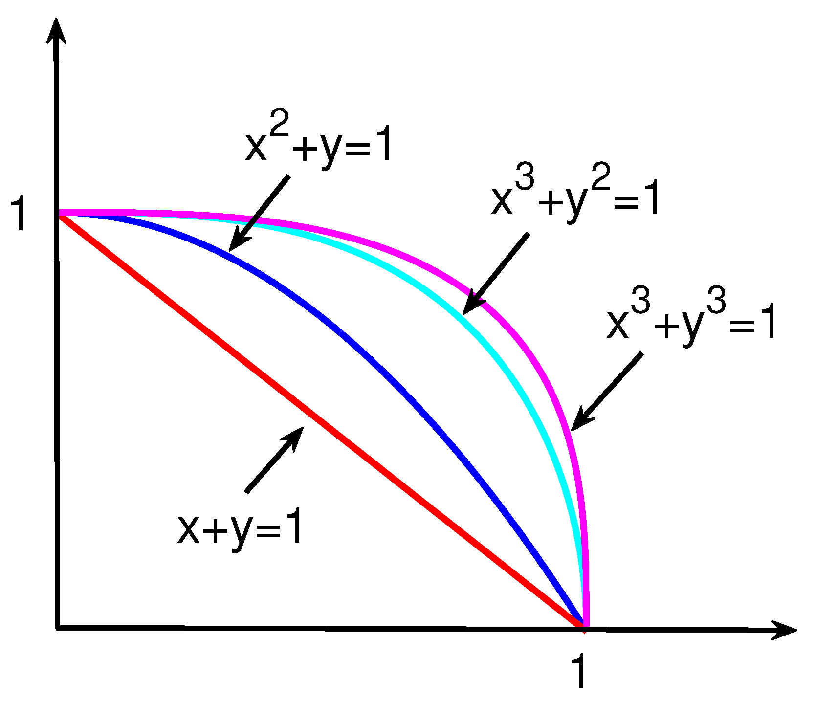
In Figure 1, we display some grade spaces of $(m,n)$-Fuzzy membership and $(m,n)$-Fuzzy non-membership.

Remark 1. 

$(m,n)$-FS coincides with

• IFS if$m=n=1$.
• PFS if$m=n=2$.
• FFS if$m=n=3$.
• q-ROFS if$m=n=q$.
• $(2,3)$-FS if $m=2$ and $n=3$.

In what follows, we compare $(m,n)$-FS with the previous generalizations of IFSs.

Proposition 1. 

• Every IFS is an $(m,n)$-FS.
• If $m\ge 2$ and $n\ge 2$, then a PFS is an $(m,n)$-FS.
• If $m\ge 3$ and $n\ge 3$, then a FFS is an $(m,n)$-FS.
• If $m\ge q$ and $n\ge q$, then a q-ROFS is an $(m,n)$-FS.
• If $m\ge 2$ and $n\ge 3$, then a $(2,3)$-FS is an $(m,n)$-FS.

Proof. 

Straightforward.    □

As we show in examples given in Section 2 that the converses of the relationships given in Proposition 1 are false, in general.

Definition 6. 

Let $E_1=({\beta }_{E_1},{\lambda }_{E_1})$ and $E_2=({\beta }_{E_2},{\lambda }_{E_2})$ be $(m,n)$-Fuzzy sets on U. Then

• $E_1\cup E_2=(max\{{\beta }_{E_1},{\beta }_{E_2}\},min\{{\lambda }_{E_1},{\lambda }_{E_2}\})$.
• $E_1\cap E_2=(min\{{\beta }_{E_1},{\beta }_{E_2}\},max\{{\lambda }_{E_1},{\lambda }_{E_2}\})$.
• $E_1^c=({\lambda }_{E_1}^{\frac{n}{m}},{\beta }_{E_1}^{\frac{m}{n}})$.

Note that ${\left({\lambda }_{E_1}^{\frac{n}{m}}\right)}^m+{\left({\beta }_{E_1}^{\frac{m}{n}}\right)}^n={\lambda }_{E_1}^n+{\beta }_{E_1}^m\le 1$, so $E_1^c$ is an $(m,n)$-Fuzzy set. It is obvious that ${\left(E^c\right)}^c=({\beta }_E,{\lambda }_E)$.

For more illustration we provide the following example.

Example 1. 

Assume that $E_1=(0.9,0.3)$ and $E_2=(0.7,0.8)$ are both $(4,2)$-FSs on U. Then

• $E_1\cup E_2=(max\{{\beta }_{E_1},{\beta }_{E_2}\},min\{{\lambda }_{E_1},{\lambda }_{E_2}\})$$=\left(max\right\{0.9,0.7\},min\{0.3,0.8\left\}\right)=(0.9,0.3)$.
• $E_1\cap E_2=(min\{{\beta }_{E_1},{\beta }_{E_2}\},max\{{\lambda }_{E_1},{\lambda }_{E_2}\})$$=\left(min\right\{0.9,0.7\},max\{0.3,0.8\left\}\right)=(0.7,0.8)$.
• $E_1^c=(0.3,0.9)$and$E_2^c=(0.8,0.7)$.

Proposition 2. 

Let$E_1=({\beta }_{E_1},{\lambda }_{E_1})$and$E_2=({\beta }_{E_2},{\lambda }_{E_2})$be$(m,n)$-FSs on U. Then

• $E_1\cup E_2=E_2\cup E_1$.
• $E_1\cap E_2=E_2\cap E_1$.

Proof. 

Straightforward.    □

Proposition 3. 

Let$E_1=({\beta }_{E_1},{\lambda }_{E_1})$,$E_2=({\beta }_{E_2},{\lambda }_{E_2})$and$E_3=({\beta }_{E_3},{\lambda }_{E_3})$be$(m,n)$-FSs on U. Then

• $E_1\cup (E_2\cup E_3)=(E_1\cup E_2)\cup E_3$.
• $E_1\cap (E_2\cap E_3)=(E_1\cap E_2)\cap E_3$.

Proof. 

For the three $(m,n)$-FSs $E_1,E_2$ and $E_3$ on U, according to Definition 6, we obtain:

• $\begin{array}{c}{E}_1\cup (E_2\cup E_3)=({\beta }_{E_1},{\lambda }_{E_1})\cup (max\{{\beta }_{E_2},{\beta }_{E_3}\},min\{{\lambda }_{E_2},{\lambda }_{E_3}\})\\ =(max\{{\beta }_{E_1},max\{{\beta }_{E_2},{\beta }_{E_3}\}\},min\{{\lambda }_{E_1},min\{{\lambda }_{E_2},{\lambda }_{E_3}\}\})\\ =(max\{max\{{\beta }_{E_1},{\beta }_{E_2}\},{\beta }_{E_3}\},min\{min\{{\lambda }_{E_1},{\lambda }_{E_2}\},{\lambda }_{E_3}\})\\ =(max\{{\beta }_{E_1},{\beta }_{E_2}\},min\{{\lambda }_{E_1},{\lambda }_{E_2}\})\cup ({\beta }_{E_3},{\lambda }_{E_3})\\ =(E_1\cap E_2)\cup E_3\end{array}$.
• Similar to 1 above.

   □

Theorem 1. 

Let$E_1=({\beta }_{E_1},{\lambda }_{E_1})$,$E_2=({\beta }_{E_2},{\lambda }_{E_2})$and$E_3=({\beta }_{E_3},{\lambda }_{E_3})$be$(m,n)$-FSs. Then

1. 

$(E_1\cup E_2)\cap E_3=(E_1\cap E_3)\cup (E_2\cap E_3)$.

2. 

$(E_1\cap E_2)\cup E_3=(E_1\cup E_3)\cap (E_2\cup E_3)$.

Proof. 

For the three $(m,n)$-FSs $E_1,E_2$ and $E_3$, according to Definition 6, we obtain:

• $(E_1\cup E_2)\cap E_3=(max\{{\beta }_{E_1},{\beta }_{E_2}\},min\{{\lambda }_{E_1},{\lambda }_{E_2}\})\cap ({\beta }_{E_3},{\lambda }_{E_3})$
  $=(min\{max\{{\beta }_{E_1},{\beta }_{E_2}\},{\beta }_{E_3}\},max\{min\{{\lambda }_{E_1},{\lambda }_{E_2}\},{\lambda }_{E_3}\})$. And,
  $(E_1\cap E_3)\cup (E_2\cap E_3)=(min\{{\beta }_{E_1},{\beta }_{E_3}\},max\{{\lambda }_{E_1},{\lambda }_{E_3}\})\cup (min\{{\beta }_{E_2},{\beta }_{E_3}\},max\{{\lambda }_{E_2},{\lambda }_{E_3}\})$
  $=(max\{min\{{\beta }_{E_1},{\beta }_{E_3}\},min\{{\beta }_{E_2},{\beta }_{E_3}\}\},min\{max\{{\lambda }_{E_1},{\lambda }_{E_3}\},max\{{\lambda }_{E_2},{\lambda }_{E_3}\}\})$. Then,

  $$min\{max\{{\beta }_{E_1},{\beta }_{E_2}\},{\beta }_{E_3}\}=\left\{\begin{array}{cc}\hfill {\beta }_{E_2}\hfill & \hfill \mathrm{if}{\beta }_{E_1}\le {\beta }_{E_2}\le {\beta }_{E_3},\hfill \\ \hfill {\beta }_{E_1}\hfill & \hfill \mathrm{if}{\beta }_{E_2}\le {\beta }_{E_1}\le {\beta }_{E_3},\hfill \\ \hfill {\beta }_{E_3}\hfill & \hfill \mathrm{if}{\beta }_{E_1}\le {\beta }_{E_3}\le {\beta }_{E_2},\hfill \\ \hfill {\beta }_{E_3}\hfill & \hfill \mathrm{if}{\beta }_{E_3}\le {\beta }_{E_1}\le {\beta }_{E_2},\hfill \\ \hfill {\beta }_{E_3}\hfill & \hfill \mathrm{if}{\beta }_{E_2}\le {\beta }_{E_3}\le {\beta }_{E_1},\hfill \\ \hfill {\beta }_{E_3}\hfill & \hfill \mathrm{if}{\beta }_{E_3}\le {\beta }_{E_2}\le {\beta }_{E_1},\hfill \end{array}\right.$$

  $$max\{min\{{\lambda }_{E_1},{\lambda }_{E_2}\},{\lambda }_{E_3}\}=\left\{\begin{array}{cc}\hfill {\lambda }_{E_3}\hfill & \hfill \mathrm{if}{\lambda }_{E_1}\le {\lambda }_{E_2}\le {\lambda }_{E_3},\hfill \\ \hfill {\lambda }_{E_3}\hfill & \hfill \mathrm{if}{\lambda }_{E_2}\le {\lambda }_{E_1}\le {\lambda }_{E_3},\hfill \\ \hfill {\lambda }_{E_3}\hfill & \hfill \mathrm{if}{\lambda }_{E_1}\le {\lambda }_{E_3}\le {\lambda }_{E_2},\hfill \\ \hfill {\lambda }_{E_1}\hfill & \hfill \mathrm{if}{\lambda }_{E_3}\le {\lambda }_{E_1}\le {\lambda }_{E_2},\hfill \\ \hfill {\lambda }_{E_3}\hfill & \hfill \mathrm{if}{\lambda }_{E_2}\le {\lambda }_{E_3}\le {\lambda }_{E_1},\hfill \\ \hfill {\lambda }_{E_2}\hfill & \hfill \mathrm{if}{\lambda }_{E_3}\le {\lambda }_{E_2}\le {\lambda }_{E_1},\hfill \end{array}\right.$$

  $$max\{min\{{\beta }_{E_1},{\beta }_{E_3}\},min\{{\beta }_{E_2},{\beta }_{E_3}\}\}=\left\{\begin{array}{cc}\hfill {\beta }_{E_2}\hfill & \hfill \mathrm{if}{\beta }_{E_1}\le {\beta }_{E_2}\le {\beta }_{E_3},\hfill \\ \hfill {\beta }_{E_1}\hfill & \hfill \mathrm{if}{\beta }_{E_2}\le {\beta }_{E_1}\le {\beta }_{E_3},\hfill \\ \hfill {\beta }_{E_3}\hfill & \hfill \mathrm{if}{\beta }_{E_1}\le {\beta }_{E_3}\le {\beta }_{E_2},\hfill \\ \hfill {\beta }_{E_3}\hfill & \hfill \mathrm{if}{\beta }_{E_3}\le {\beta }_{E_1}\le {\beta }_{E_2},\hfill \\ \hfill {\beta }_{E_3}\hfill & \hfill \mathrm{if}{\beta }_{E_2}\le {\beta }_{E_3}\le {\beta }_{E_1},\hfill \\ \hfill {\beta }_{E_3}\hfill & \hfill \mathrm{if}{\beta }_{E_3}\le {\beta }_{E_2}\le {\beta }_{E_1},\hfill \end{array}\right.$$

  $$min\{max\{{\lambda }_{E_1},{\lambda }_{E_3}\},max\{{\lambda }_{E_2},{\lambda }_{E_3}\}\}=\left\{\begin{array}{cc}\hfill {\lambda }_{E_3}\hfill & \hfill \mathrm{if}{\lambda }_{E_1}\le {\lambda }_{E_2}\le {\lambda }_{E_3},\hfill \\ \hfill {\lambda }_{E_3}\hfill & \hfill \mathrm{if}{\lambda }_{E_2}\le {\lambda }_{E_1}\le {\lambda }_{E_3},\hfill \\ \hfill {\lambda }_{E_3}\hfill & \hfill \mathrm{if}{\lambda }_{E_1}\le {\lambda }_{E_3}\le {\lambda }_{E_2},\hfill \\ \hfill {\lambda }_{E_1}\hfill & \hfill \mathrm{if}{\lambda }_{E_3}\le {\lambda }_{E_1}\le {\lambda }_{E_2},\hfill \\ \hfill {\lambda }_{E_3}\hfill & \hfill \mathrm{if}{\lambda }_{E_2}\le {\lambda }_{E_3}\le {\lambda }_{E_1},\hfill \\ \hfill {\lambda }_{E_2}\hfill & \hfill \mathrm{if}{\lambda }_{E_3}\le {\lambda }_{E_2}\le {\lambda }_{E_1}.\hfill \end{array}\right.$$
  Thus, $min\{max\{{\beta }_{E_1},{\beta }_{E_2}\},{\beta }_{E_3}\}=max\{min\{{\beta }_{E_1},{\beta }_{E_3}\},min\{{\beta }_{E_2},{\beta }_{E_3}\}\}$ and $max\{min$$\{{\lambda }_{E_1},{\lambda }_{E_2}\},{\lambda }_{E_3}\}=min\{max\{{\lambda }_{E_1},{\lambda }_{E_3}\},max\{{\lambda }_{E_2},{\lambda }_{E_3}\}\}$. Hence, $(E_1\cup E_2)\cap E_3=(E_1\cap E_3)\cup (E_2\cap E_3)$.
• $(E_1\cap E_2)\cup E_3=(min\{{\beta }_{E_1},{\beta }_{E_2}\},max\{{\lambda }_{E_1},{\lambda }_{E_2}\})\cup ({\beta }_{E_3},{\lambda }_{E_3})$
  $=(max\{min\{{\beta }_{E_1},{\beta }_{E_2}\},{\beta }_{E_3}\},min\{max\{{\lambda }_{E_1},{\lambda }_{E_2}\},{\lambda }_{E_3}\})$. And,
  $(E_1\cup E_3)\cap (E_2\cup E_3)=(max\{{\beta }_{E_1},{\beta }_{E_3}\},min\{{\lambda }_{E_1},{\lambda }_{E_3}\})\cap (max\{{\beta }_{E_2},{\beta }_{E_3}\},min\{{\lambda }_{E_2},{\lambda }_{E_3}\})$
  $=(min\{max\{{\beta }_{E_1},{\beta }_{E_3}\},max\{{\beta }_{E_2},{\beta }_{E_3}\}\},max\{min\{{\lambda }_{E_1},{\lambda }_{E_3}\},min\{{\lambda }_{E_2},{\lambda }_{E_3}\}\})$. Then,

  $$max\{min\{{\beta }_{E_1},{\beta }_{E_2}\},{\beta }_{E_3}\}=\left\{\begin{array}{cc}\hfill {\beta }_{E_3}\hfill & \hfill \mathrm{if}{\beta }_{E_1}\le {\beta }_{E_2}\le {\beta }_{E_3},\hfill \\ \hfill {\beta }_{E_3}\hfill & \hfill \mathrm{if}{\beta }_{E_2}\le {\beta }_{E_1}\le {\beta }_{E_3},\hfill \\ \hfill {\beta }_{E_3}\hfill & \hfill \mathrm{if}{\beta }_{E_1}\le {\beta }_{E_3}\le {\beta }_{E_2},\hfill \\ \hfill {\beta }_{E_1}\hfill & \hfill \mathrm{if}{\beta }_{E_3}\le {\beta }_{E_1}\le {\beta }_{E_2},\hfill \\ \hfill {\beta }_{E_3}\hfill & \hfill \mathrm{if}{\beta }_{E_2}\le {\beta }_{E_3}\le {\beta }_{E_1},\hfill \\ \hfill {\beta }_{E_2}\hfill & \hfill \mathrm{if}{\beta }_{E_3}\le {\beta }_{E_2}\le {\beta }_{E_1},\hfill \end{array}\right.$$

  $$min\{max\{{\lambda }_{E_1},{\lambda }_{E_2}\},{\lambda }_{E_3}\}=\left\{\begin{array}{cc}\hfill {\lambda }_{E_2}\hfill & \hfill \mathrm{if}{\lambda }_{E_1}\le {\lambda }_{E_2}\le {\lambda }_{E_3},\hfill \\ \hfill {\lambda }_{E_1}\hfill & \hfill \mathrm{if}{\lambda }_{E_2}\le {\lambda }_{E_1}\le {\lambda }_{E_3},\hfill \\ \hfill {\lambda }_{E_3}\hfill & \hfill \mathrm{if}{\lambda }_{E_1}\le {\lambda }_{E_3}\le {\lambda }_{E_2},\hfill \\ \hfill {\lambda }_{E_3}\hfill & \hfill \mathrm{if}{\lambda }_{E_3}\le {\lambda }_{E_1}\le {\lambda }_{E_2},\hfill \\ \hfill {\lambda }_{E_3}\hfill & \hfill \mathrm{if}{\lambda }_{E_2}\le {\lambda }_{E_3}\le {\lambda }_{E_1},\hfill \\ \hfill {\lambda }_{E_3}\hfill & \hfill \mathrm{if}{\lambda }_{E_3}\le {\lambda }_{E_2}\le {\lambda }_{E_1},\hfill \end{array}\right.$$

  $$min\{max\{{\beta }_{E_1},{\beta }_{E_3}\},max\{{\beta }_{E_2},{\beta }_{E_3}\}\}=\left\{\begin{array}{cc}\hfill {\beta }_{E_3}\hfill & \hfill \mathrm{if}{\beta }_{E_1}\le {\beta }_{E_2}\le {\beta }_{E_3},\hfill \\ \hfill {\beta }_{E_3}\hfill & \hfill \mathrm{if}{\beta }_{E_2}\le {\beta }_{E_1}\le {\beta }_{E_3},\hfill \\ \hfill {\beta }_{E_3}\hfill & \hfill \mathrm{if}{\beta }_{E_1}\le {\beta }_{E_3}\le {\beta }_{E_2},\hfill \\ \hfill {\beta }_{E_1}\hfill & \hfill \mathrm{if}{\beta }_{E_3}\le {\beta }_{E_1}\le {\beta }_{E_2},\hfill \\ \hfill {\beta }_{E_3}\hfill & \hfill \mathrm{if}{\beta }_{E_2}\le {\beta }_{E_3}\le {\beta }_{E_1},\hfill \\ \hfill {\beta }_{E_2}\hfill & \hfill \mathrm{if}{\beta }_{E_3}\le {\beta }_{E_2}\le {\beta }_{E_1},\hfill \end{array}\right.$$

  $$max\{min\{{\lambda }_{E_1},{\lambda }_{E_3}\},min\{{\lambda }_{E_2},{\lambda }_{E_3}\}\}=\left\{\begin{array}{cc}\hfill {\lambda }_{E_2}\hfill & \hfill if{\lambda }_{E_1}\le {\lambda }_{E_2}\le {\lambda }_{E_3},\hfill \\ \hfill {\lambda }_{E_1}\hfill & \hfill \mathrm{if}{\lambda }_{E_2}\le {\lambda }_{E_1}\le {\lambda }_{E_3},\hfill \\ \hfill {\lambda }_{E_3}\hfill & \hfill \mathrm{if}{\lambda }_{E_1}\le {\lambda }_{E_3}\le {\lambda }_{E_2},\hfill \\ \hfill {\lambda }_{E_3}\hfill & \hfill \mathrm{if}{\lambda }_{E_3}\le {\lambda }_{E_1}\le {\lambda }_{E_2},\hfill \\ \hfill {\lambda }_{E_3}\hfill & \hfill \mathrm{if}{\lambda }_{E_2}\le {\lambda }_{E_3}\le {\lambda }_{E_1},\hfill \\ \hfill {\lambda }_{E_3}\hfill & \hfill \mathrm{if}{\lambda }_{E_3}\le {\lambda }_{E_2}\le {\lambda }_{E_1}.\hfill \end{array}\right.$$
  Thus, $max\{min\{{\beta }_{E_1},{\beta }_{E_2}\},{\beta }_{E_3}\}=min\{max\{{\beta }_{E_1},{\beta }_{E_3}\},max\{{\beta }_{E_2},{\beta }_{E_3}\}\}$ and $min\{max$$\{{\lambda }_{E_1},{\lambda }_{E_2}\},{\lambda }_{E_3}\}=max\{min\{{\lambda }_{E_1},{\lambda }_{E_3}\},min\{{\lambda }_{E_2},{\lambda }_{E_3}\}\}$. Hence, $(E_1\cap E_2)\cup E_3=(E_1\cup E_3)\cap (E_2\cup E_3)$.

   □

Theorem 2. 

Let $E_1=({\beta }_{E_1},{\lambda }_{E_1})$ and $E_2=({\beta }_{E_2},{\lambda }_{E_2})$ be $(m,n)$-FSs on U. Then

1. 

${(E_1\cup E_2)}^c=E_1^c\cap E_2^c$.

2. 

${(E_1\cap E_2)}^c=E_1^c\cup E_2^c$.

Proof.  

• For the $(m,n)$-FSs $E_1$ and $E_2$, according to Definition 6, we obtain ${(E_1\cup E_2)}^c={(max\{{\beta }_{E_1},{\beta }_{E_2}\},min\{{\lambda }_{E_1},{\lambda }_{E_2}\})}^c$
  $=(min\{{\left({\lambda }_{E_1}\right)}^{\frac{n}{m}},{\left({\lambda }_{E_2}\right)}^{\frac{n}{m}}\},max\{{\left({\beta }_{E_1}\right)}^{\frac{m}{n}},{\left({\beta }_{E_2}\right)}^{\frac{m}{n}}\})$
  $=({\left({\lambda }_{E_1}\right)}^{\frac{n}{m}},{\left({\beta }_{E_1}\right)}^{\frac{m}{n}})\cap {\left({\lambda }_{E_2}\right)}^{\frac{n}{m}},{\left({\beta }_{E_2}\right)}^{\frac{m}{n}})$
  $=E_1^c\cap E_2^c$.
• Similar to 1.

   □

Definition 7. 

Let $\{E_i=({\beta }_{E_i},{\lambda }_{E_i}):i\in I\}$ be a family of $(m,n)$-FSs on U. Then

1. 

$\underset{i\in I}{\cup }{E}_i=(sup\{{\beta }_{E_i}:i\in I\},inf\{{\lambda }_{E_i}:i\in I\})$.

2. 

$\underset{i\in I}{\cap }{E}_i=(inf\{{\beta }_{E_i}:i\in I\},sup\{{\lambda }_{E_i}:i\in I\})$.

In what follows we define the functions of score and accuracy with respect to $(m,n)$-FSs which we apply to rank $(m,n)$-FSs.

Proposition 4. 

For any$(m,n)$-FS$E=({\beta }_E,{\lambda }_E)$on U, the value of${\beta }_E^m-{\lambda }_E^n$lies in the closed interval$[-1,1]$.

Proof. 

For any $(m,n)$-FS E, we have ${\beta }_E^m+{\lambda }_E^n\le 1$. This implies that ${\beta }_E^m-{\lambda }_E^n\le {\beta }_E^m\le 1$ and ${\beta }_E^m-{\lambda }_E^n\ge -{\lambda }_E^n\ge -1$. Hence, $-1\le {\beta }_E^m-{\lambda }_E^n\le 1$, as required.    □

Definition 8. 

The score function$score:I^{(m,n)-FS}\to [-1,1]$is given by the formula$score\left(E\right)={\beta }_E^m-{\lambda }_E^n$for every$(m,n)$-FS$E=({\beta }_E,{\lambda }_E)$.

Definition 9. 

Let$E_1=({\beta }_{E_1},{\lambda }_{E_1})$and$E_2=({\beta }_{E_2},{\lambda }_{E_2})$be$(m,n)$-FSs. We say that

(i) 

If$score\left(E_1\right)>score\left(E_2\right)$, then$E_1\succ E_2$.

(ii) 

If$score\left(E_1\right)<score\left(E_2\right)$, then$E_1\prec E_2$.

(iii) 

If$score\left(E_1\right)=score\left(E_2\right)$, then$E_1\simeq E_2$.

Example 2. 

Let$E_1=(0.65,0.75)$and$E_2=(0.82,0.55)$be$(6,4)$-FSs. We obtain$score\left(E_1\right)=-0.240987359$and$acc\left(E_2\right)=0.212500421$. Hence,

Definition 10. 

The accuracy function$acc:I^{(m,n)-FS}\to [0,1]$is given by the formula$acc\left(E\right)={\beta }_E^m+{\lambda }_E^n$for every$(m,n)$-FS$E=({\beta }_E,{\lambda }_E)$.

Definition 11. 

Let$E_1=({\beta }_{E_1},{\lambda }_{E_1})$and$E_2=({\beta }_{E_2},{\lambda }_{E_2})$be$(m,n)$-FSs. We say that

(i) 

If$score\left(E_1\right)>score\left(E_2\right)$, then$E_1\succ E_2$.

(ii) 

If$score\left(E_1\right)<score\left(E_2\right)$, then$E_1\prec E_2$.

(iii) 

If$score\left(E_1\right)=score\left(E_2\right)$, then

1. 

If$acc\left(E_1\right)>acc\left(E_2\right)$, then$E_1\succ E_2$.

2. 

If$acc\left(E_1\right)<acc\left(E_2\right)$, then$E_1\prec E_2$.

3. 

If$acc\left(E_1\right)=acc\left(E_2\right)$, then$E_1=E_2$.

Example 3. 

Consider$E_1=(0.4,0.064)$and$E_2=(0.7,0.343)$$(3,1)$-FSs, and $E_3=(0.6,0.8)$and$E_4=(0.9,0.4)$are$(2,5)$-FSs on$U=\left\{a\right\}$. Obviously,$score\left(E_1\right)=score\left(E_2\right)=0$, whereas$acc\left(E_2\right)={\beta }_{E_2}^3+{\lambda }_{E_2}=0.686>acc\left(E_1\right)={\beta }_{E_1}^3+{\lambda }_{E_1}=0.128$. Therefore,$E_2\succ E_1$. Also,$score\left(E_3\right)=0.03232$and$score\left(E_4\right)=0.79976$, which means that$E_4\succ E_3$.

Definition 12. 

Let$E_1=({\beta }_{E_1},{\lambda }_{E_1})$and$E_2=({\beta }_{E_2},{\lambda }_{E_2})$be$(m,n)$-FSs on U. A natural quasi-ordering on the$(m,n)$-FSs is defined as follows.$E_1\ge E_2$iff${\beta }_{E_1}\ge {\beta }_{E_2}$and${\lambda }_{E_1}\le {\lambda }_{E_2}$.

4. Aggregation of $(\mathit{m},\mathit{n})$-Fuzzy Sets with Applications

     We dedicate this section to present some novel types of operations on $(m,n)$-Fuzzy sets and explore their master features. Then, we define new kinds of aggregation operators with respect to $(m,n)$-Fuzzy sets and illustrate the relationships between them. Some illustrative examples are provided.

4.1. Some Operations on $(m,n)$-FSs

In this part, we introduce some operations over the class of $(m,n)$-Fuzzy sets, and show the relationships between them.

Definition 13. 

For two $(m,n)$-FSs on U $E_1=({\beta }_{E_1},{\lambda }_{E_1})$ and $E_2=({\beta }_{E_2},{\lambda }_{E_2})$ and a positive real number ($\nu >0$) ν, the following operations are defined.

1. 

$E_1\oplus E_2=\left(\sqrt[m]{{\beta }_{E_1}^m+{\beta }_{E_2}^m-{\beta }_{E_1}^m{\beta }_{E_2}^m},{\lambda }_{E_1}{\lambda }_{E_2}\right)$.

2. 

$E_1\otimes E_2=\left({\beta }_{E_1}{\beta }_{E_2},\sqrt[n]{{\lambda }_{E_1}^n+{\lambda }_{E_2}^n-{\lambda }_{E_1}^n{\lambda }_{E_2}^n}\right)$.

3. 

$\nu E_1=\left(\sqrt[m]{1-{(1-{\beta }_{E_1}^m)}^{\nu }},{\lambda }_{E_1}^{\nu }\right)$.

4. 

$E_1^{\nu }=\left({\beta }_{E_1}^{\nu },\sqrt[n]{1-{(1-{\lambda }_{E_1}^n)}^{\nu }}\right)$.

Example 4. 

Suppose that $E_1=(0.2,0.9)$ and $E_2=(0.65,0.45)$ are $(3,4)$-FSs on $U=\left\{a\right\}$, and $\nu =2$. Then

1. 

$E_1\oplus E_2=\left(\sqrt[3]{{\beta }_{E_1}^3+{\beta }_{E_2}^3-{\beta }_{E_1}^3{\beta }_{E_2}^3},{\lambda }_{E_1}{\lambda }_{E_2}\right)$

     $=\left(\sqrt[3]{0.2^3+0.{65}^3-{\left(0.2\right)}^3{\left(0.65\right)}^3},\left(0.9\right)\left(0.45\right)\right)\approx (0.654546,0.405)$.

2. 

$E_1\otimes E_2=\left({\beta }_{E_1}{\beta }_{E_2},\sqrt[4]{{\lambda }_{E_1}^4+{\lambda }_{E_2}^4-{\lambda }_{E_1}^4{\lambda }_{E_2}^4}\right)$

     $=\left(\left(0.2\right)\left(0.65\right),\sqrt[4]{{\left(0.9\right)}^4+{\left(0.45\right)}^4-{\left(0.9\right)}^4{\left(0.45\right)}^4}\right)\approx (0.13,0.904798)$.

3. 

$2E_1=\left(\sqrt[3]{1-{(1-{\beta }_{E_1}^3)}^2},{\lambda }_{E_1}^2\right)=\left(\sqrt[3]{1-{(1-0.2^3)}^2},0.9^2\right)\approx (0.251648,0.81)$.

4. 

$E_1^2=\left({\beta }_{E_1}^2,\sqrt[4]{1-{(1-{\lambda }_{E_1}^4)}^2}\right)=\left(0.2^2,\sqrt[4]{1-{(1-0.9^4)}^2}\right)\approx (0.04,0.969023)$.

Theorem 3. 

If $E_1=({\beta }_{E_1},{\lambda }_{E_1})$ and $E_2=({\beta }_{E_2},{\lambda }_{E_2})$ are $(m,n)$-FSs on U, then $E_1\oplus E_2$ and $E_1\otimes E_2$ are $(m,n)$-FSs.

Proof. 

For $(m,n)$-FSs $E_1=({\beta }_{E_1},{\lambda }_{E_1})$ and $E_2=({\beta }_{E_2},{\lambda }_{E_2})$, we obtain $0\le {\beta }_{E_1}^m+{\lambda }_{E_1}^n\le 1$ and $0\le {\beta }_{E_2}^m+{\lambda }_{E_2}^n\le 1$.

Then, we have ${\beta }_{E_1}^m\ge {\beta }_{E_1}^m{\beta }_{E_2}^m,{\beta }_{E_2}^m\ge {\beta }_{E_1}^m{\beta }_{E_2}^m,0\le {\beta }_{E_1}^m{\beta }_{E_2}^m\le 1\mathrm{and}$ and ${\lambda }_{E_1}^n\ge {\lambda }_{E_1}^n{\lambda }_{E_2}^n$, ${\lambda }_{E_2}^n\ge {\lambda }_{E_1}^n{\lambda }_{E_2}^n$, $0\le {\lambda }_{E_1}^n{\lambda }_{E_2}^n\le 1$.

This implies that $\sqrt[m]{{\beta }_{E_1}^m+{\beta }_{E_2}^m-{\beta }_{E_1}^m{\beta }_{E_2}^m}\ge 0$.

Since ${\beta }_{E_2}^m\le 1$ and $0\le 1-{\beta }_{E_1}^m$, ${\beta }_{E_2}^m(1-{\beta }_{E_1}^m)\le (1-{\beta }_{E_1}^m)$, we get that ${\beta }_{E_1}^m+{\beta }_{E_2}^m-{\beta }_{E_1}^m{\beta }_{E_2}^m\le 1$. Thus, $\sqrt[m]{{\beta }_{E_1}^m+{\beta }_{E_2}^m-{\beta }_{E_1}^m{\beta }_{E_2}^m}\le 1$. It is clear that $0\le {\lambda }_{E_1}^n\le 1-{\beta }_{E_1}^m$ and $0\le {\lambda }_{E_2}^n\le 1-{\beta }_{E_2}^m$.

Now, ${\left(\sqrt[m]{{\beta }_{E_1}^m+{\beta }_{E_2}^m-{\beta }_{E_1}^m{\beta }_{E_2}^m}\right)}^m+{\lambda }_{E_1}^n{\lambda }_{E_2}^n\le {\beta }_{E_1}^m+{\beta }_{E_2}^m-{\beta }_{E_1}^m{\beta }_{E_2}^m+(1-{\beta }_{E_1}^m)(1-{\beta }_{E_2}^m)=1$.

Hence, $0\le {\left(\sqrt[m]{{\beta }_{E_1}^m+{\beta }_{E_2}^m-{\beta }_{E_1}^m{\beta }_{E_2}^2}\right)}^m+{\lambda }_{E_1}^n{\lambda }_{E_2}^n\le 1$ which means that $E_1\oplus E_2$ is an $(m,n)$-FS.

Following similar arguments, we prove that $E_1\otimes E_2$ is an $(m,n)$-FS.    □

Theorem 4. 

Let $E=({\beta }_E,{\lambda }_E)$ be an $(m,n)$-FS on U and ν be a positive real number. Then, $\nu E$ and $E^{\nu }$ are $(m,n)$-FSs.

Proof. 

Since $0\le {\beta }_E^m\le 1$, $0\le {\lambda }_E^n\le 1$ and $0\le {\left({\beta }_E\right)}^m+{\lambda }_E^n\le 1$, we find

$0\le {\lambda }_E^n\le 1-{\beta }_E^m$

$\Rightarrow 0\le {(1-{\beta }_E^m)}^{\nu }$

$\Rightarrow 1-{(1-{\beta }_E^m)}^{\nu }\le 1$

$\Rightarrow 0\le \sqrt[m]{1-{(1-{\beta }_E^m)}^{\nu }}\le \sqrt[m]{1}=1$.

It is clear that $0\le {\lambda }_E^{\nu }\le 1$, then we get

$0\le {\left(\sqrt[m]{1-{(1-{\beta }_E^m)}^{\nu }}\right)}^m+{\left({\lambda }_E^{\nu }\right)}^n\le 1-{(1-{\beta }_E^m)}^{\nu }+{(1-{\beta }_E^m)}^{\nu }=1$.

In a similar way, we get

$0\le {\left({\beta }_E^{\nu }\right)}^m+1-{(1-{\lambda }_E)}^{\nu }\le 1$.

Hence, $\nu E$ and $E^{\nu }$ are $(m,n)$-FSs.    □

Theorem 5. 

Let$E_1=({\beta }_{E_1},{\lambda }_{E_1})$and$E_2=({\beta }_{E_2},{\lambda }_{E_2})$be$(m,n)$-FSs on U. Then

1. 

$E_1\oplus E_2=E_2\oplus E_1$.

2. 

$E_1\otimes E_2=E_2\otimes E_1$.

Proof. 

From Definition 13, we obtain:

• $$\begin{gathered} E_1\oplus E_2=\left(\sqrt[m]{{\beta }_{E_1}^m+{\beta }_{E_2}^m-{\beta }_{E_1}^m{\beta }_{E_2}^m},{\lambda }_{E_1}{\lambda }_{E_2}\right) \\ \left(\sqrt[m]{{\beta }_{E_2}^m+{\beta }_{E_1}^m-{\beta }_{E_2}^m{\beta }_{E_1}^m},{\lambda }_{E_2}{\lambda }_{E_1}\right)=E_2\oplus E_1 \end{gathered}$$.
• $$\begin{gathered} E_1\otimes E_2=\left({\beta }_{E_1}{\beta }_{E_2},\sqrt[n]{{\lambda }_{E_1}^n+{\lambda }_{E_2}^n-{\lambda }_{E_1}^n{\lambda }_{E_2}^n}\right) \\ =\left({\beta }_{E_2}{\beta }_{E_1},\sqrt[n]{{\lambda }_{E_2}^n+{\lambda }_{E_1}^n-{\lambda }_{E_2}^n{\lambda }_{E_1}^n}\right)=E_2\otimes E_1 \end{gathered}$$.

   □

Theorem 6. 

Let$E=({\beta }_E,{\lambda }_E)$,$E_1=({\beta }_{E_1},{\lambda }_{E_1})$and$E_2=({\beta }_{E_2},{\lambda }_{E_2})$be$(m,n)$-FSs on U. Then

1. 

$\nu (E_1\oplus E_2)=\nu E_1\oplus \nu E_2$for$\nu >0$.

2. 

$({\nu }_1+{\nu }_2)E={\nu }_{1}E\oplus {\nu }_{2}E$for${\nu }_1,{\nu }_2>0$.

3. 

${(E_1\otimes E_2)}^{\nu }=E_1^{\nu }\otimes E_2^{\nu }$for$\nu >0$.

4. 

$E^{({\nu }_1+{\nu }_2)}=E^{{\nu }_1}\otimes E^{{\nu }_2}$for${\nu }_1,{\nu }_2>0$.

Proof.  

• $\nu (E_1\oplus E_2)=\nu \left(\sqrt[m]{{\beta }_{E_1}^m+{\beta }_{E_2}^m-{\beta }_{E_1}^m{\beta }_{E_2}^m},{\lambda }_{E_1}{\lambda }_{E_2}\right)=\left(\sqrt[m]{1-(1-{\beta }_{E_1}^m-{\beta }_{E_2}^m+{\beta }_{E_1}^m{\beta }_{E_2}^m}{)}^{\nu },{\left({\lambda }_{E_1}{\lambda }_{E_2}\right)}^{\nu }\right)$
  $=\left(\sqrt[m]{1-{(1-{\beta }_{E_1}^m)}^{\nu }{(1-{\beta }_{E_2}^m)}^{\nu }},{\lambda }_{E_1}^{\nu }{\lambda }_{E_2}^{\nu }\right)$.
  And $$\begin{gathered} \nu E_1\oplus \nu E_2=\left(\sqrt[m]{1-{(1-{\beta }_{E_1}^m)}^{\nu }},{\lambda }_{E_1}^{\nu }\right)\oplus \left(\sqrt{1-{(1-{\beta }_{E_2}^m)}^{\nu }},{\lambda }_{E_2}^{\nu }\right) \\ =\left(\sqrt[m]{1-{(1-{\beta }_{E_1}^m)}^{\nu }+1-{(1-{\beta }_{E_2}^m)}^{\nu }-(1-{(1-{\beta }_{E_1}^m)}^{\nu })(1-{(1-{\beta }_{E_2}^m)}^{\nu })},{\lambda }_{E_1}^{\nu }{\lambda }_{E_2}^{\nu }\right) \\ =\left(\sqrt[m]{1-{(1-{\beta }_{E_1}^m)}^{\nu }{(1-{\beta }_{E_2}^m)}^{\nu }},{\lambda }_{E_1}^{\nu }{\lambda }_{E_2}^{\nu }\right)=\nu (E_1\oplus E_2) \end{gathered}$$.
• $$\begin{gathered} ({\nu }_1+{\nu }_2)E=({\nu }_1+{\nu }_2)({\beta }_E,{\lambda }_E) \\ =\left(\sqrt[m]{1-{(1-{\beta }_E^m)}^{{\nu }_1+{\nu }_2}},{\lambda }_E^{{\nu }_1+{\nu }_2}\right) \\ =\left(\sqrt[m]{1-{(1-{\beta }_E^m)}^{{\nu }_1}{(1-{\beta }_E^m)}^{{\nu }_2}},{\lambda }_E^{{\nu }_1+{\nu }_2}\right) \\ =\left(\sqrt[m]{1-{(1-{\beta }_E^m)}^{{\nu }_1}+1-{(1-{\beta }_E^m)}^{{\nu }_2}-(1-{(1-{\beta }_E^m)}^{{\nu }_1})(1-{(1-{\beta }_E^m)}^{{\nu }_2})},{\lambda }_E^{{\nu }_1}{\lambda }_E^{{\nu }_2}\right) \\ =\left(\sqrt[m]{1-{(1-{\beta }_E^m)}^{{\nu }_1}},{\lambda }_E^{{\nu }_1}\right)\oplus \left(\sqrt[m]{1-{(1-{\beta }_E^m)}^{{\nu }_2}},{\lambda }_E^{{\nu }_2}\right) \\ ={\nu }_{1}E\oplus {\nu }_{2}E \end{gathered}$$.
• $$\begin{gathered} {(E_1\otimes E_2)}^{\nu }={\left({\beta }_{E_1}{\beta }_{E_2},\sqrt[n]{{\lambda }_{E_1}^n+{\lambda }_{E_2}^n-{\lambda }_{E_1}^n{\lambda }_{E_2}^n}\right)}^{\nu } \\ =\left({\left({\beta }_{E_1}{\beta }_{E_2}\right)}^{\nu },\sqrt[n]{1-{(1-{\lambda }_{E_1}^n-{\lambda }_{E_2}^n+{\lambda }_{E_1}^n{\lambda }_{E_2}^n)}^{\nu }}\right) \\ =\left({\beta }_{E_1}^{\nu }{\beta }_{E_2}^{\nu },\sqrt[n]{1-{(1-{\lambda }_{E_1}^n)}^{\nu }{(1-{\lambda }_{E_2}^n)}^{\nu }}\right) \\ =\left({\beta }_{E_1}^{\nu },\sqrt[n]{1-{(1-{\lambda }_{E_1}^n)}^{\nu }}\right)\otimes \left({\beta }_{E_2}^{\nu },\sqrt[n]{1-{(1-{\lambda }_{E_2}^n)}^{\nu }}\right) \\ =E_1^{\nu }\otimes E_2^{\nu } \end{gathered}$$.
• $$\begin{gathered} E^{{\nu }_1}\otimes E^{{\nu }_2}=\left({\beta }_E^{{\nu }_1},\sqrt[n]{1-{(1-{\lambda }_E^n)}^{{\nu }_1}}\right)\otimes \left({\beta }_E^{{\nu }_2},\sqrt[n]{1-{(1-{\lambda }_E^n)}^{{\nu }_2}}\right) \\ =\left({\beta }_E^{{\nu }_1+{\nu }_2},\sqrt[n]{1-{(1-{\lambda }_E^n)}^{{\nu }_1}+1-{(1-{\lambda }_E^n)}^{{\nu }_2}-(1-{(1-{\lambda }_E^n)}^{{\nu }_1})(1-{(1-{\lambda }_E^n)}^{{\nu }_2})}\right) \\ =\left({\beta }_E^{{\nu }_1+{\nu }_2},\sqrt[n]{1-{(1-{\lambda }_E^n)}^{{\nu }_1+{\nu }_2}}\right) \\ =E^{({\nu }_1+{\nu }_2)} \end{gathered}$$.

   □

Theorem 7. 

Let$E_1=({\beta }_{E_1},{\lambda }_{E_1})$and$E_2=({\beta }_{E_2},{\lambda }_{E_2})$be$(m,n)$-FSs on U, and $\nu >0$. Then

1. 

$\nu (E_1\cup E_2)=\nu E_1\cup \nu E_2$.

2. 

${(E_1\cup E_2)}^{\nu }=E_1^{\nu }\cup E_2^{\nu }$.

Proof. 

For the two $(m,n)$-FSs $E_1$ and $E_2$, and $\nu >0$, according to definitions 6 and 13, we obtain

• $$\begin{gathered} \nu (E_1\cup E_2)=\nu (max\{{\beta }_{E_1},{\beta }_{E_2}\},min\{{\lambda }_{E_1},{\lambda }_{E_2}\}) \\ =\left(\sqrt[m]{1-{(1-max\{{\beta }_{E_1}^m,{\beta }_{E_2}^m\})}^{\nu }},min\{{\lambda }_{E_1}^{\nu },{\lambda }_{E_2}^{\nu }\}\right) \end{gathered}$$.
  And $\nu E_1\cup \nu E_2=\left(\sqrt[m]{1-{(1-{\beta }_{E_1}^m)}^{\nu }},{\lambda }_{E_1}^{\nu }\right)\cup \left(\sqrt[m]{1-{(1-{\beta }_{E_2}^m)}^{\nu }},{\lambda }_{E_2}^{\nu }\right)$
  $$\begin{gathered} =\left(max\{\sqrt[m]{1-{(1-{\beta }_{E_1}^m)}^{\nu }},\sqrt{1-{(1-{\beta }_{E_2}^m)}^{\nu }}\},min\{{\lambda }_{E_1}^{\nu },{\lambda }_{E_2}^{\nu }\}\right) \\ =\left(\sqrt{1-{(1-max\{{\beta }_{E_1}^m,{\beta }_{E_2}^m\})}^{\nu }},min\{{\lambda }_{E_1}^{\nu },{\lambda }_{E_2}^{\nu }\}\right)=\nu (E_1\cup E_2) \end{gathered}$$.
• Similar to 1.

   □

Theorem 8. 

Let$E=({\beta }_E,{\lambda }_E)$,$E_1=({\beta }_{E_1},{\lambda }_{E_1})$and$E_2=({\beta }_{E_2},{\lambda }_{E_2})$be$(m,n)$-FSs on U, and $\nu >0$. Then

1. 

${(E_1\oplus E_2)}^c=E_1^c\otimes E_2^c$.

2. 

${(E_1\otimes E_2)}^c=E_1^c\oplus E_2^c$.

3. 

${\left(E^c\right)}^{\nu }={\left(\nu E\right)}^c$.

4. 

$\nu {\left(E\right)}^c={\left(E^{\nu }\right)}^c$.

Proof.  

• $$\begin{gathered} {(E_1\oplus E_2)}^c={\left(\sqrt[m]{{\beta }_{E_1}^m+{\beta }_{E_2}^m-{\beta }_{E_1}^m{\beta }_{E_2}^m},{\lambda }_{E_1}{\lambda }_{E_2}\right)}^c \\ =\left(\sqrt[m]{{\lambda }_{E_1}^n{\lambda }_{E_2}^n},\sqrt[n]{{\beta }_{E_1}^m+{\beta }_{E_2}^m-{\beta }_{E_1}^m{\beta }_{E_2}^m}\right) \\ =\left(\sqrt[m]{{\lambda }_{E_1}^n}\sqrt[m]{{\lambda }_{E_2}^n},\sqrt[n]{{\beta }_{E_1}^m+{\beta }_{E_2}^m-{\beta }_{E_1}^m{\beta }_{E_2}^m}\right) \\ =(\sqrt[m]{{\lambda }_{E_1}^n},{\beta }_{E_1}^m)\otimes (\sqrt[n]{{\lambda }_{E_2}^n},{\beta }_{E_2}^m) \\ =E_1^c\otimes E_2^c \end{gathered}$$.
• $$\begin{gathered} {(E_1\otimes E_2)}^c={\left({\beta }_{E_1}{\beta }_{E_2},\sqrt[n]{{\lambda }_{E_1}^n+{\lambda }_{E_2}^n-{\lambda }_{E_1}^n{\lambda }_{E_2}^n}\right)}^c \\ =\left(\sqrt[m]{{\lambda }_{E_1}^n+{\lambda }_{E_2}^n-{\lambda }_{E_1}^n{\lambda }_{E_2}^n},\sqrt[n]{{\beta }_{E_1}^m{\beta }_{E_2}^m}\right) \\ =\left(\sqrt[m]{{\lambda }_{E_1}^n+{\lambda }_{E_2}^n-{\lambda }_{E_1}^n{\lambda }_{E_2}^n},\sqrt[n]{{\beta }_{E_1}^m}\sqrt[n]{{\beta }_{E_2}^m}\right) \\ =(\sqrt[m]{{\lambda }_{E_1}^n},\sqrt[n]{{\beta }_{E_1}^m})\oplus (\sqrt[m]{{\lambda }_{E_2}^n},\sqrt[n]{{\beta }_{E_2}^m}) \end{gathered}$$
  $=E_1^c\oplus E_2^c$.
• $$\begin{gathered} {\left(E^c\right)}^{\nu }={(\sqrt[m]{{\lambda }_E^n},\sqrt[n]{{\beta }_E^m})}^{\nu } \\ =\left({\left(\sqrt[m]{{\lambda }_E^n}\right)}^{\nu },\sqrt[n]{1-{(1-{\beta }_E^m)}^{\nu }}\right) \\ ={\left(\sqrt[m]{1-{(1-{\beta }_E^m)}^{\nu }},{\lambda }_E^{\nu }\right)}^c \\ ={\left(\nu E\right)}^c \end{gathered}$$.
• $$\begin{gathered} \nu {\left(E\right)}^c=\nu (\sqrt[m]{{\lambda }_E^n},\sqrt[n]{{\beta }_E^m})=\left(\sqrt[m]{1-{(1-{\lambda }_E^n)}^{\nu }},{\left(\sqrt[n]{{\beta }_E^m}\right)}^{\nu }\right)={\left({\beta }_E^{\nu },\sqrt[n]{1-{(1-{\lambda }_E^n)}^{\nu }}\right)}^c \\ ={\left(E^{\nu }\right)}^c \end{gathered}$$.

   □

Theorem 9. 

Let$E_1=({\beta }_{E_1},{\lambda }_{E_1})$,$E_2=({\beta }_{E_2},{\lambda }_{E_2})$and$E_3=({\beta }_{E_3},{\lambda }_{E_3})$be$(m,n)$-FSs on U. Then

1. 

$(E_1\cap E_2)\oplus E_3=(E_1\oplus E_3)\cap (E_2\oplus E_3)$.

2. 

$(E_1\cup E_2)\oplus E_3=(E_1\oplus E_3)\cup (E_2\oplus E_3)$.

3. 

$(E_1\cap E_2)\otimes E_3=(E_1\otimes E_3)\cap (E_2\otimes E_3)$.

4. 

$(E_1\cup E_2)\otimes E_3=(E_1\otimes E_3)\cup (E_2\otimes E_3)$.

Proof.  

• $$\begin{gathered} (E_1\cap E_2)\oplus E_3=(min\{{\beta }_{E_1},{\beta }_{E_2}\},max\{{\lambda }_{E_1},{\lambda }_{E_2}\})\oplus ({\beta }_{E_3},{\lambda }_{E_3}) \\ =\left(\sqrt[m]{min\{{\beta }_{E_1}^m,{\beta }_{E_2}^m\}+{\beta }_{E_3}^m-{\beta }_{E_3}^{m}min\{{\beta }_{E_1}^m,{\beta }_{E_2}^m\}},max\{{\lambda }_{E_1},{\lambda }_{E_2}\}{\lambda }_{E_3}\right) \\ =\left(\sqrt[m]{(1-{\beta }_{E_3}^m)min\{{\beta }_{E_1}^m,{\beta }_{E_2}^m\}+{\beta }_{E_3}^m},max\{{\lambda }_{E_1}{\lambda }_{E_3},{\lambda }_{E_2}{\lambda }_{E_3}\}\right) \end{gathered}$$.
  And $(E_1\oplus E_3)\cap (E_2\oplus E_3)$
  $$\begin{gathered} =\left(\sqrt[m]{{\beta }_{E_1}^m+{\beta }_{E_3}^m-{\beta }_{E_1}^m{\beta }_{E_3}^m},{\lambda }_{E_1}{\lambda }_{E_3}\right)\cap \left(\sqrt{{\beta }_{E_2}^m+{\beta }_{E_3}^m-{\beta }_{E_2}^m{\beta }_{E_3}^m},{\lambda }_{E_2}{\lambda }_{E_3}\right) \\ =\left(min\{\sqrt[m]{{\beta }_{E_1}^m+{\beta }_{E_3}^m-{\beta }_{E_1}^m{\beta }_{E_3}^m},\sqrt{{\beta }_{E_2}^m+{\beta }_{E_3}^m-{\beta }_{E_2}^m{\beta }_{E_3}^m}\},max\{{\lambda }_{E_1}{\lambda }_{E_3},{\lambda }_{E_2}{\lambda }_{E_3}\}\right) \\ =\left(min\{\sqrt[m]{(1-{\beta }_{E_3}^m){\beta }_{E_1}^m+{\beta }_{E_3}^m},\sqrt[m]{(1-{\beta }_{E_3}^m){\beta }_{E_2}^m+{\beta }_{E_3}^m}\},max\{{\lambda }_{E_1}{\lambda }_{E_3},{\lambda }_{E_2}{\lambda }_{E_3}\}\right) \\ =\left(\sqrt[m]{(1-{\beta }_{E_3}^m)min\{{\beta }_{E_1}^m,{\beta }_{E_2}^m\}+{\beta }_{E_3}^m},max\{{\lambda }_{E_1}{\lambda }_{E_3},{\lambda }_{E_2}{\lambda }_{E_3}\}\right) \end{gathered}$$.
  Hence, $(E_1\cap E_2)\oplus E_3=(E_1\oplus E_3)\cap (E_2\oplus E_3)$.
• Similar to 1.
• $$\begin{gathered} (E_1\cap E_2)\otimes E_3=(min\{{\beta }_{E_1},{\beta }_{E_2}\},max\{{\lambda }_{E_1},{\lambda }_{E_2}\})\otimes E_3 \\ =\left(min\{{\beta }_{E_1},{\beta }_{E_2}\}{\beta }_{E_3},\sqrt[n]{max\{{\lambda }_{E_1}^n,{\lambda }_{E_2}^n\}+{\lambda }_{E_3}^n-{\lambda }_{E_3}^{n}max\{{\lambda }_{E_1}^n,{\lambda }_{E_2}^n}\}\right) \\ =\left(min\{{\beta }_{E_1}{\beta }_{E_3},{\beta }_{E_2}{\beta }_{E_3}\},\sqrt[n]{(1-{\lambda }_{E_3}^n)max\{{\lambda }_{E_1}^n,{\lambda }_{E_2}^n\}+{\lambda }_{E_3}^n}\right) \end{gathered}$$.
  And $(E_1\otimes E_3)\cap (E_2\otimes E_3)=\left({\beta }_{E_1}{\beta }_{E_3},\sqrt[n]{{\lambda }_{E_1}^n+{\lambda }_{E_3}^n-{\lambda }_{E_1}^n{\lambda }_{E_3}^n}\right)$ $\cap \left({\beta }_{E_2}{\beta }_{E_3},\sqrt[n]{{\lambda }_{E_2}^n+{\lambda }_{E_3}^n-{\lambda }_{E_2}^n{\lambda }_{E_3}^n}\right)$
  $=\left({\beta }_{E_1}{\beta }_{E_3},\sqrt[n]{(1-{\lambda }_{E_3}^n){\lambda }_{E_1}^n+{\lambda }_{E_3}^n}\right)\cap \left({\beta }_{E_2}{\beta }_{E_3},\sqrt[n]{(1-{\lambda }_{E_3}^n){\lambda }_{E_2}^n+{\lambda }_{E_3}^n}\right)$
  $$\begin{gathered} =\left(min\{{\beta }_{E_1}{\beta }_{E_3},{\beta }_{E_2}{\beta }_{E_3}\},max\left\{\sqrt[n]{(1-{\lambda }_{E_3}^n){\lambda }_{E_1}^n+{\lambda }_{E_3}^n},\sqrt[n]{(1-{\lambda }_{E_3}^n){\lambda }_{E_2}^n+{\lambda }_{E_3}^n}\right\}\right) \\ =\left(min\{{\beta }_{E_1}{\beta }_{E_3},{\beta }_{E_2}{\beta }_{E_3}\},\sqrt[n]{(1-{\lambda }_{E_3}^n)max\{{\lambda }_{E_1}^n,{\lambda }_{E_2}^n\}+{\lambda }_{E_3}^n}\right) \end{gathered}$$.
  Hence, $(E_1\cap E_2)\otimes E_3=(E_1\otimes E_3)\cap (E_2\otimes E_3)$.
• Similar to 3.

□

Theorem 10. 

Let$E_1=({\beta }_{E_1},{\lambda }_{E_1})$,$E_2=({\beta }_{E_2},{\lambda }_{E_2})$and$E_3=({\beta }_{E_3},{\lambda }_{E_3})$be$(m,n)$-FSs on U. Then

1. 

$E_1\oplus E_2\oplus E_3=E_1\oplus E_3\oplus E_2$.

2. 

$E_1\otimes E_2\otimes E_3=E_1\otimes E_3\otimes E_2$.

Proof.  

• $$\begin{gathered} E_1\oplus E_2\oplus E_3 \\ =({\beta }_{E_1},{\lambda }_{E_1})\oplus ({\beta }_{E_2},{\lambda }_{E_2})\oplus ({\beta }_{E_3},{\lambda }_{E_3}) \\ =\left(\sqrt[m]{{\beta }_{E_1}^m+{\beta }_{E_2}^m-{\beta }_{E_1}^m{\beta }_{E_2}^m},{\lambda }_{E_1}{\lambda }_{E_2}\right)\oplus ({\beta }_{E_3},{\lambda }_{E_3}) \\ =\left(\sqrt[m]{{\beta }_{E_1}^m+{\beta }_{E_2}^m-{\beta }_{E_1}^m{\beta }_{E_2}^m+{\beta }_{E_3}^m-{\beta }_{E_3}^m({\beta }_{E_1}^m+{\beta }_{E_2}^m-{\beta }_{E_1}^m{\beta }_{E_2}^m)},{\lambda }_{E_1}{\lambda }_{E_2}{\lambda }_{E_3}\right) \\ =\left(\sqrt[m]{{\beta }_{E_1}^m+{\beta }_{E_2}^m+{\beta }_{E_3}^m-{\beta }_{E_1}^m{\beta }_{E_2}^m-{\beta }_{E_1}^m{\beta }_{E_3}^m-{\beta }_{E_2}^m{\beta }_{E_3}^m+{\beta }_{E_1}^m{\beta }_{E_2}^m{\beta }_{E_3}^m},{\lambda }_{E_1}{\lambda }_{E_2}{\lambda }_{E_3}\right) \\ =\left(\sqrt[m]{{\beta }_{E_1}^m+{\beta }_{E_3}^m-{\beta }_{E_1}^m{\beta }_{E_3}^m+{\beta }_{E_2}^m-{\beta }_{E_2}^m({\beta }_{E_1}^m+{\beta }_{E_3}^m-{\beta }_{E_1}^m{\beta }_{E_3}^m)},{\lambda }_{E_1}{\lambda }_{E_2}{\lambda }_{E_3}\right) \\ =\left(\sqrt[m]{{\beta }_{E_1}^m+{\beta }_{E_3}^m-{\beta }_{E_1}^m{\beta }_{E_3}^m},{\lambda }_{E_1}{\lambda }_{E_3}\right)\oplus ({\beta }_{E_2},{\lambda }_{E_2}) \\ =E_1\oplus E_3\oplus E_2 \end{gathered}$$.
• Similar to 1.

□

4.2. Aggregation of $(m,n)$-Fuzzy Sets

In this subsection, we discuss some well-known aggregation operators with respect to the environment of $(m,n)$-Fuzzy sets. We investigate their main properties and reveal the relationships between them.

Definition 14. 

Let$E_j=({\beta }_{E_j},{\lambda }_{E_j})$$(j=1,2,...,s)$be a family of$(m,n)$-FNs on U, and $w={(w_1,w_2,...,w_s)}^T$be a weight vector of$E_j$with$w_j>0$and${\sum }_{j=1}^s{w}_j=1$. Then

1. 

an$(m,n)$-Fuzzy weighted average ($(m,n)$-FWA) operator is given by$(m,n)$-$FWA(E_1,E_2,...,E_s)=({\sum }_{j=1}^s{w}_j{\beta }_{E_j},{\sum }_{j=1}^s{w}_j{\lambda }_{E_j})$.

2. 

an$(m,n)$-Fuzzy weighted geometric ($(m,n)$-FWG) operator is given by$(m,n)$-$FWG(E_1,E_2,...,E_s)=({\prod }_{j=1}^s{\beta }_{E_j}^{w_j},{\prod }_{j=1}^s{\lambda }_{E_j}^{w_j})$.

3. 

an$(m,n)$-Fuzzy weighted power average ($(m,n)$-FWPA) operator is given by$(m,n)$-$FWPA(E_1,E_2,...,E_m)=({\left({\sum }_{j=1}^s{w}_j{\beta }_{E_j}^m\right)}^{\frac{1}{m}},{\left({\sum }_{j=1}^s{w}_j{\lambda }_{E_j}^n\right)}^{\frac{1}{n}})$.

4. 

an$(m,n)$-Fuzzy weighted power geometric ($(m,n)$-FWPG) operator is given by$(m,n)$-$FWPG(E_1,E_2,...,E_s)=({(1-{\prod }_{j=1}^s{(1-{\beta }_{E_j}^m)}^{w_j})}^{\frac{1}{m}},{(1-{\prod }_{j=1}^s{(1-{\lambda }_{E_j}^n)}^{w_j})}^{\frac{1}{n}})$.

Remark 2. 

In general, the values obtained from the operators presented in the above definition need not be an $(m,n)$-FS.

Example below illustrates how these aggregations operators are calculated.

Example 5. 

Let$E_1=(0.4,0.9),E_2=(0.6,0.6),E_3=(0.3,0.8)$, and $E_4=(0.8,0.5)$be$(1,5)$-FNs on$U=\left\{a\right\}$, and let$w={(0.1,0.2,0.4,0.3)}^T$be a weight vector of$E_j(j=1,2,3,4)$. Then

1. 

$(1,5)$-$FWA(E_1,E_2,E_3,E_4)=(0.1\times 0.4+0.2\times 0.6+0.4\times 0.3+0.3\times 0.8,0.1\times 0.9+0.2\times 0.6+0.4\times 0.8+0.3\times 0.5)=(0.52,0.68)$.

2. 

$(1,5)$-$FWG(E_1,E_2,E_3,E_4)=(0.4^{0.1}\times 0.6^{0.2}\times 0.3^{0.4}\times 0.8^{0.3},0.9^{0.1}\times 0.6^{0.2}\times 0.8^{0.4}\times 0.5^{0.3})\approx (0.476005,0.663715)$.

3. 

$(1,5)$-$FWPA(E_1,E_2,E_3,E_4)=(0.1\times 0.4+0.2\times 0.6+0.4\times 0.3+0.3\times 0.8,{(0.1\times 0.9^5+0.2\times 0.6^5+0.4\times 0.8^5+0.3\times 0.5^5)}^{\frac{1}{5}})\approx (0.52,0.735372)$.

4. 

$(1,5)$-$FWPG(E_1,E_2,E_3,E_4)=(1-[{(1-0.4)}^{0.1}\times {(1-0.6)}^{0.2}\times {(1-0.3)}^{0.4}\times {(1-0.8)}^{0.3}]),$$[1-[{(1-0.9^5)}^{0.1}\times {(1-0.6^5)}^{0.2}\times {(1-0.8^5)}^{0.4}\times {(1-0.5^5)}^{0.3})]{]}^{\frac{1}{5}}\approx (0.423229,0.751394)$.

Theorem 11. 

Let$E_j=({\beta }_{E_j},{\lambda }_{E_j})(i=1,2,...,s)$be a family of$(m,n)$-FNs on U,$E=({\beta }_E,{\lambda }_E)$be an$(m,n)$-FN and$w={(w_1,w_2,...,w_s)}^T$be a weight vector of$E_j$with${\sum }_{j=1}^s{w}_j=1$. Then

1. 

$(m,n)$-$FWA(E_1\oplus E,E_2\oplus E,...,E_s\oplus E)\ge (m,n)$-$FWA(E_1\otimes E,E_2\otimes E,...,E_s\otimes E)$.

2. 

$(m,n)$-$FWG(E_1\oplus E,E_2\oplus E,...,E_s\oplus E)\ge (m,n)$-$FWG(E_1\otimes E,E_2\otimes E,...,E_s\otimes E)$.

3. 

$(m,n)$-$FWPA(E_1\oplus E,E_2\oplus E,...,E_s\oplus E)\ge (m,n)$-$FWPA(E_1\otimes E,E_2\otimes E,...,E_s\otimes E)$.

4. 

$(m,n)$-$FWPG(E_1\oplus E,E_2\oplus E,...,E_s\oplus E)\ge (m,n)$-$FWPG(E_1\otimes E,E_2\otimes E,...,E_s\otimes E)$.

Proof. 

We suffice by proving 1 and 4.

(1) For any $E_j=({\beta }_{E_j},{\lambda }_{E_j})$$(j=1,2,\dots ,s)$ and $E=({\beta }_E,{\lambda }_E)$, we obtain $\sqrt[m]{{\beta }_{E_j}^m+{\beta }_E^m-{\beta }_{E_j}^m{\beta }_E^m}\ge \sqrt[m]{2{\beta }_{E_j}^m{\beta }_E^m-{\beta }_{E_j}^m{\beta }_E^m}={\beta }_{E_j}{\beta }_E$, and  $\sqrt[n]{{\lambda }_{E_j}^n+{\lambda }_E^n-{\lambda }_{E_j}^n{\lambda }_E^n}\ge \sqrt[n]{2{\lambda }_{E_j}^n{\lambda }_E^n-{\lambda }_{E_j}^n{\lambda }_E^n}={\lambda }_{E_j}{\lambda }_E$.

That is,

$$\sum _{j=1}^s{w}_j\sqrt[m]{{\beta }_{E_j}^m+{\beta }_E^m-{\beta }_{E_j}^m{\beta }_E^m}\ge \sum _{j=1}^s{w}_j{\beta }_{E_j}{\beta }_E$$

(1)

and

$$\sum _{j=1}^s{w}_j\sqrt[n]{{\lambda }_{E_j}^n+{\lambda }_E^n-{\lambda }_{E_j}^n{\lambda }_E^n}\ge \sum _{j=1}^s{w}_j{\lambda }_{E_j}{\lambda }_E.$$

(2)

It follows from Definitions 13 and 14 that $(m,n)$-$FWA(E_1\oplus E,E_2\oplus E,...,E_s\oplus E)=({\sum }_{j=1}^s{w}_j\sqrt[m]{{\beta }_{E_j}^m+{\beta }_E^m-{\beta }_{E_j}^m{\beta }_E^m},{\sum }_{j=1}^s{w}_j{\lambda }_{E_j}{\lambda }_E)$

and

$(m,n)$-$FWA(E_1\otimes E,E_2\otimes E,...,E_s\otimes E)=({\sum }_{j=1}^s{w}_j{\beta }_{E_j}{\beta }_E,{\sum }_{j=1}^s{w}_j\sqrt[n]{{\lambda }_{E_j}^n+{\lambda }_E^n-{\lambda }_{E_j}^n{\lambda }_E^n})$.

Hence, from (1) and (2), we complete the proof.

(4) For any $E_j=({\beta }_{E_j},{\lambda }_{E_j})(j=1,2,...,s)$ and $E=({\beta }_E,{\lambda }_E)$, we obtain

$$\begin{gathered} {\beta }_{E_j}^m+{\beta }_E^m-{\beta }_{E_j}^m{\beta }_E^m\ge 2{\beta }_{E_j}^m{\beta }_E^m-{\beta }_{E_j}^m{\beta }_E^m={\beta }_{E_j}^m{\beta }_E^m \\ \Rightarrow 1-({\beta }_{E_j}^m+{\beta }_E^m-{\beta }_{E_j}^m{\beta }_E^m)\le 1-{\beta }_{E_j}^m{\beta }_E^m \\ \Rightarrow {(1-({\beta }_{E_j}^m+{\beta }_E^m-{\beta }_{E_j}^m{\beta }_E^m))}^{w_j}\le {(1-{\beta }_{E_j}^m{\beta }_E^m)}^{w_j} \\ \Rightarrow {\prod }_{j=1}^s{(1-({\beta }_{E_j}^m+{\beta }_E^m-{\beta }_{E_j}^m{\beta }_E^m))}^{w_j}\le {\prod }_{j=1}^s{(1-{\beta }_{E_j}^m{\beta }_E^m)}^{w_j} \end{gathered}$$$\Rightarrow 1-{\prod }_{j=1}^s{(1-({\beta }_{E_j}^m+{\beta }_E^m-{\beta }_{E_j}^m{\beta }_E^m))}^{w_j}\ge 1-{\prod }_{j=1}^s{(1-{\beta }_{E_j}^m{\beta }_E^m)}^{w_j}$.

Similarly, $\Rightarrow 1-{\prod }_{j=1}^s{(1-({\lambda }_{E_j}^n+{\lambda }_E^n-{\lambda }_{E_j}^n{\lambda }_E^n))}^{w_j}\ge 1-{\prod }_{j=1}^s{(1-{\lambda }_{E_j}^n{\lambda }_E^n)}^{w_j}$.

According to items 1 and 2 of Definition 13, we have $(m,n)$-$FWPG(E_1\oplus E,E_2\oplus E,...,E_s\oplus E)=({(1-{\prod }_{j=1}^s{(1-({\beta }_{E_j}^m+{\beta }_E^m-{\beta }_{E_j}^m{\beta }_E^m))}^{w_j})}^{\frac{1}{m}},{(1-{\prod }_{j=1}^s{(1-{\lambda }_{E_j}^n{\lambda }_E^n)}^{w_j})}^{\frac{1}{n}})$, and  $(m,n)$-$FWPG(E_1\otimes E,E_2\otimes E,...,E_s\otimes E)=({(1-{\prod }_{j=1}^s{(1-{\beta }_{E_j}^m{\beta }_E^m)}^{w_j})}^{\frac{1}{m}},{(1-{\prod }_{j=1}^s{(1-({\lambda }_{E_j}^n+{\lambda }_E^n-{\lambda }_{E_j}^n{\lambda }_E^n))}^{w_j})}^{\frac{1}{n}})$.

Hence, $(m,n)$-$FWPG(E_1\oplus E,E_2\oplus E,...,E_s\oplus E)\ge (m,n)$-$FWPG(E_1\otimes E,E_2\otimes E,\dots ,$$E_s\otimes E)$, as required.    □

Theorem 12. 

Let$E_j=({\beta }_{E_j},{\lambda }_{E_j})$and${\Gamma }_j=({\beta }_{{\Gamma }_j},{\lambda }_{{\Gamma }_j})(j=1,2,...,s)$be two families of$(m,n)$-FSs on U, and $w={(w_1,w_2,...,w_s)}^T$be a weight vector of them with${\sum }_{j=1}^s{w}_j=1$. Then

1. 

$(m,n)$-$FWA(E_1\oplus {\Gamma }_1,E_2\oplus {\Gamma }_2,...,E_s\oplus {\Gamma }_s)\ge (m,n)$-$FWA(E_1\otimes {\Gamma }_1,E_2\otimes {\Gamma }_2,...,E_s\otimes {\Gamma }_s)$.

2. 

$(m,n)$-$FWG(E_1\oplus {\Gamma }_1,E_2\oplus {\Gamma }_2,...,E_s\oplus {\Gamma }_s)\ge (m,n)$-$FWG(E_1\otimes {\Gamma }_1,E_2\otimes {\Gamma }_2,...,E_s\otimes {\Gamma }_s)$.

3. 

$(m,n)$-$FWPA(E_1\oplus {\Gamma }_1,E_2\oplus {\Gamma }_2,...,E_s\oplus {\Gamma }_s)\ge (m,n)$-$FWPA(E_1\otimes {\Gamma }_1,E_2\otimes {\Gamma }_2,...,E_s\otimes {\Gamma }_s)$.

4. 

$(m,n)$-$FWPG(E_1\oplus {\Gamma }_1,E_2\oplus {\Gamma }_2,...,E_s\oplus {\Gamma }_s)\ge (m,n)$-$FWPG(E_1\otimes {\Gamma }_1,E_2\otimes {\Gamma }_2,...,E_s\otimes {\Gamma }_s)$.

Proof. 

We suffice by proving 1.

(1) For any $E_j=({\beta }_{E_j},{\lambda }_{E_j})$ and ${\Gamma }_j=({\beta }_{{\Gamma }_j},{\lambda }_{{\Gamma }_j})$$(j=1,2,\dots ,s)$, we can get $\sqrt[m]{{\beta }_{E_j}^m+{\beta }_{{\Gamma }_j}^m-{\beta }_{E_j}^m{\beta }_{{\Gamma }_j}^m}\ge \sqrt[m]{2{\beta }_{E_j}^m{\beta }_{{\Gamma }_j}^m-{\beta }_{E_j}^m{\beta }_{{\Gamma }_j}^m}={\beta }_{E_j}{\beta }_{{\Gamma }_j}$.

That is, ${\sum }_{j=1}^s{w}_j\sqrt[m]{{\beta }_{E_j}^m+{\beta }_{{\Gamma }_j}^m-{\beta }_{E_j}^m{\beta }_{{\Gamma }_j}^m}\ge {\sum }_{j=1}^s{w}_j{\beta }_{E_j}{\beta }_{{\Gamma }_j}$.

Similarly,

${\sum }_{j=1}^s{w}_j\sqrt[n]{{\lambda }_{E_j}^n+{\lambda }_{{\Gamma }_j}^n-{\lambda }_{E_j}^n{\lambda }_{{\Gamma }_j}^n}\ge {\sum }_{j=1}^s{w}_j{\lambda }_{E_j}{\lambda }_{{\Gamma }_j}$.

By items 1 and 2 of Definition 13, we have $(m,n)-FWA(E_1\oplus {\Gamma }_1,E_2\oplus {\Gamma }_2,...,E_s\oplus {\Gamma }_s)=({\sum }_{j=1}^s{w}_j\sqrt[m]{{\beta }_{E_j}^m+{\beta }_{{\Gamma }_j}^m-{\beta }_{E_j}^m{\beta }_{{\Gamma }_j}^m},{\sum }_{j=1}^s{w}_j{\lambda }_{E_j}{\lambda }_{{\Gamma }_j})$ and $(m,n)-FWA(E_1\otimes {\Gamma }_1,E_2\otimes {\Gamma }_2,...,E_s\otimes {\Gamma }_s)=({\sum }_{j=1}^s{w}_j{\beta }_{E_j}{\beta }_{{\Gamma }_j},{\sum }_{j=1}^s{w}_j\sqrt[n]{{\lambda }_{E_j}^n+{\lambda }_{{\Gamma }_j}^n-{\lambda }_{E_j}^n{\lambda }_{{\Gamma }_j}^n})$.

Hence, $(m,n)$-$FWA(E_1\oplus {\Gamma }_1,E_2\oplus {\Gamma }_2,...,E_s\oplus {\Gamma }_s)\ge (m,n)$-$FWA(E_1\otimes {\Gamma }_1,E_2\otimes {\Gamma }_2,\dots ,E_s\otimes {\Gamma }_s)$, as required.    □

Theorem 13. 

Let$E_j=({\beta }_{E_j},{\lambda }_{E_j})(j=1,2,...,s)$be a family of$(m,n)$-FNs on U, and $w={(w_1,w_2,...,w_s)}^T$be a weight vector of$E_j$with${\sum }_{j=1}^s{w}_j=1$and$\nu \ge 1$. Then

1. 

$(m,n)$-$FWA(\nu E_1,\nu E_2,...,\nu E_s)\ge (m,n)$-$FWA(E_1^{\nu },E_2^{\nu },...,E_s^{\nu })$.

2. 

$(m,n)$-$FWG(\nu E_1,\nu E_2,...,\nu E_s)\ge (m,n)$-$FWG(E_1^{\nu },E_2^{\nu },...,E_s^{\nu })$.

3. 

$(m,n)$-$FWPA(\nu E_1,\nu E_2,...,\nu E_s)\ge (m,n)$-$FWPA(E_1^{\nu },E_2^{\nu },...,E_s^{\nu })$.

4. 

$(m,n)$-$FWPG(\nu E_1,\nu E_2,...,\nu E_s)\ge (m,n)$-$FWPG(E_1^{\nu },E_2^{\nu },...,E_s^{\nu })$.

Proof. 

We suffice by proving 1.

(1) For any $E_j=({\beta }_{E_j},{\lambda }_{E_j})$$(j=1,2,\dots ,s)$, we have

$(m,n)$-$FWA(\nu E_1,\nu E_2,...,\nu E_s)=({\sum }_{j=1}^s{w}_j\sqrt[m]{1-{(1-{\beta }_{E_j}^m)}^{\nu }},{\sum }_{j=1}^s{w}_j{\lambda }_{E_j}^{\nu })$, and 

$(m,n)$-$FWA(E_1^{\nu },E_2^{\nu },...,E_s^{\nu })=({\sum }_{j=1}^s{w}_j{\beta }_{E_j}^{\nu },{\sum }_{j=1}^s{w}_j\sqrt[n]{1-{(1-{\lambda }_{E_j}^n)}^{\nu }})$.

Let $f\left({\beta }_{E_j}\right)=1-{(1-{\beta }_{E_j}^m)}^{\nu }-{\left({\beta }_{E_j}^m\right)}^{\nu }$. We demonstrate that $f\left({\beta }_{E_j}\right)\ge 0$. It follows from the Newton generalized binomial theorem that

${(1-{\beta }_{E_j}^m)}^{\nu }+{\left({\beta }_{E_j}^m\right)}^{\nu }\le {(1-{\beta }_{E_j}^m+{\beta }_{E_j}^m)}^{\nu }=1$.

This means that $f\left({\beta }_{E_j}\right)\ge 0$. Now,

$1-{(1-{\beta }_{E_j}^m)}^{\nu }-{\left({\beta }_{E_j}^m\right)}^{\nu }\ge 0$

$\Rightarrow 1-{(1-{\beta }_{E_j}^m)}^{\nu }\ge {\left({\beta }_{E_j}^m\right)}^{\nu }$

$\Rightarrow \sqrt[m]{1-{(1-{\beta }_{E_j}^m)}^{\nu }}\ge {\beta }_{E_j}^{\nu }$

$\Rightarrow {\sum }_{j=1}^s{w}_j\sqrt[m]{1-{(1-{\beta }_{E_j}^m)}^{\nu }}\ge {\sum }_{j=1}^s{w}_j{\beta }_{E_j}^{\nu }$.

Similarly,

${\sum }_{j=1}^s{w}_j\sqrt[n]{1-{(1-{\lambda }_{E_j}^n)}^{\nu }}\ge {\sum }_{j=1}^s{w}_j{\lambda }_{E_j}^{\nu }$.

Hence, $(m,n)$-$FWA(\nu E_1,\nu E_2,...,\nu E_s)\ge (m,n)$-$FWA(E_1^{\nu },E_2^{\nu },\dots ,E_s^{\nu })$, as required.    □

Theorem 14. 

Let $E_j=({\beta }_{E_j},{\lambda }_{E_j})$$(j=1,2,...,s)$ be a family of $(m,n)$-FNs on U, $E=({\beta }_E,{\lambda }_E)$ be an $(m,n)$-FN on U and $w={(w_1,w_2,...,w_s)}^T$ be a weight vector of $E_j$ with ${\sum }_{j=1}^s{w}_j=1$ and $\nu \ge 1$. Then

1. 

$(m,n)$-$FWA(\nu E_1\oplus E,\nu E_2\oplus E,...,\nu E_s\oplus E)\ge (m,n)$-$FWA(E_1^{\nu }\otimes E,E_2^{\nu }\otimes E,...,E_s^{\nu }\otimes E)$.

2. 

$(m,n)$-$FWG(\nu E_1\oplus E,\nu E_2\oplus E,...,\nu E_s\oplus E)\ge (m,n)$-$FWG(E_1^{\nu }\otimes E,E_2^{\nu }\otimes E,...,E_s^{\nu }\otimes E)$.

3. 

$(m,n)$-$FWPA(\nu E_1\oplus E,\nu E_2\oplus E,...,\nu E_s\oplus E)\ge (m,n)$-$FWPA(E_1^{\nu }\otimes E,E_2^{\nu }\otimes E,...,E_s^{\nu }\otimes E)$.

4. 

$(m,n)$-$FWPG(\nu E_1\oplus E,\nu E_2\oplus E,...,\nu E_s\oplus E)\ge (m,n)$-$FWPG(E_1^{\nu }\otimes E,E_2^{\nu }\otimes E,...,E_s^{\nu }\otimes E)$.

Proof. 

We suffice by proving 1.

(1) For any $E_j=({\beta }_{E_j},{\lambda }_{E_j})$$(j=1,2,\dots ,s)$ and $E=({\beta }_E,{\lambda }_E)$, we have

$(m,n)$-$FWA(\nu E_1\oplus E,\nu E_2\oplus E,...,\nu E_s\oplus E)=({\sum }_{j=1}^s{w}_j\sqrt[m]{1-{(1-{\beta }_{E_j}^m)}^{\nu }(1-{\beta }_E^m)},{\sum }_{j=1}^s{w}_j{\lambda }_{E_j}^{\nu }{\lambda }_E)$, and $(m,n)$-$FWA(E_1^{\nu }\otimes E,E_2^{\nu }\otimes E,...,E_s^{\nu }\otimes E)=({\sum }_{j=1}^s{w}_j{\beta }_{E_j}^{\nu }{\beta }_E,{\sum }_{j=1}^s{w}_j\sqrt[n]{1-{(1-{\lambda }_{E_j}^n)}^{\nu }(1-{\lambda }_E^n)})$.

Let $f\left({\beta }_{E_j}\right)=1-{(1-{\beta }_{E_j}^m)}^{\nu }(1-{\beta }_E^m)-{\left({\beta }_{E_j}^m\right)}^{\nu }{\beta }_E^m$. We demonstrate that $f\left({\beta }_{E_j}\right)\ge 0$. To do this, let $g\left({\beta }_{E_j}\right)={(1-{\beta }_{E_j}^m)}^{\nu }+{\left({\beta }_{E_j}^m\right)}^{\nu }$. Then

$g^{{}^{\prime }}\left({\beta }_{E_j}\right)=-2\nu {\beta }_{E_j}{(1-{\beta }_{E_j}^m)}^{\nu -1}+2\nu {\beta }_{E_j}{\left({\beta }_{E_j}^m\right)}^{\nu -1}=2\nu {\beta }_{E_j}({\left({\beta }_{E_j}^m\right)}^{\nu -1}-{(1-{\beta }_{E_j}^m)}^{\nu -1})$.

Now, if ${\beta }_{E_j}>\frac{1}{\sqrt[m]{2}}$, then $g\left({\beta }_{E_j}\right)$ is monotonic increasing and if ${\beta }_{E_j}<\frac{1}{\sqrt[m]{2}}$, then $g\left({\beta }_{E_j}\right)$ is monotonic decreasing. Therefore, $g\left({\beta }_{E_j}\right)\le g{\left({\beta }_{E_j}\right)}_{max}=max\{g\left(0\right),g\left(1\right)\}=1$. Remark that ${(1-{\beta }_{E_j}^m)}^{\nu }(1-{\beta }_E^m)+{\left({\beta }_{E_j}^m\right)}^{\nu }{\beta }_E^m\le 1$. This directly leads to that $f\left({\beta }_{E_j}\right)=1-{(1-{\beta }_{E_j}^m)}^{\nu }(1-{\beta }_E^m)-{\left({\beta }_{E_j}^m\right)}^{\nu }{\beta }_E^m\ge 0$ $\Rightarrow {\sum }_{j=1}^s{w}_j\sqrt[m]{1-{(1-{\beta }_{E_j}^m)}^{\nu }(1-{\beta }_E^m)}\ge {\sum }_{j=1}^s{w}_j{\beta }_{E_j}^{\nu }{\beta }_E$.

Similarly,

${\sum }_{j=1}^s{w}_j\sqrt[n]{1-{(1-{\lambda }_{E_j}^n)}^{\nu }(1-{\lambda }_E^n)}\ge {\sum }_{j=1}^s{w}_j{\lambda }_{E_j}^{\nu }{\lambda }_E$.

Hence, $(m,n)$-$FWA(\nu E_1\oplus E,\nu E_2\oplus E,...,\nu E_s\oplus E)\ge (m,n)$-$FWA(E_1^{\nu }\otimes E,E_2^{\nu }\otimes E,\dots ,$ $E_s^{\nu }\otimes E)$.    □

5. Decision-Making Approach Using $(\mathit{m},\mathit{n})$-FSs and Their Aggregations

     In this section, the aggregations operators, presented in the previous section, are applied to an MCDM problem. The algorithms of the proposed approach are given and an example is provided to illustrate how this approach is carried out.

5.1. Representation and Model of MCDM Problems via the Frame of $(m,n)$-FSs

MCDM problems are a fast approach to determine the best alternative(s) among the set of possible ones according to multiple criteria. To explain the followed technique, we consider the alternatives under study is the set $U=\{b_i:i=1,2,...,s\}$, and the decision maker evaluate them with respect to some criteria, say, $C=\{c_j:j=1,2,...,r\}$. Since the merits of environment of $(m,n)$-FSs to cover a huge space of grades, we consider that the estimation process of the preferences by decision maker is achieved in the environment of $(m,n)$-FNs: ${\vartheta }_{ij}={〈{\beta }_{ij},{\lambda }_{ij}〉}_{i\times j}$, where $0\le {\beta }_{ij}^m+{\lambda }_{ij}^n\le 1$ and ${\beta }_{ij},{\lambda }_{ij}\in [0,1]$ for all $i=1,2,...,s$ and $j=1,2,...,r$ such that ${\beta }_{ij}$ and ${\lambda }_{ij}$, respectively, represent the degree that the alternative $b_i$ satisfies and does not satisfy the attribute $c_j$. Thus, MCDM problems can be concisely expressed in an $(m,n)$-Fuzzy decision matrix $\mathcal{A}={\left({\vartheta }_{ij}\right)}_{s\times r}={〈{\beta }_{ij},{\lambda }_{ij}〉}_{s\times r}$.

The next steps illustrate how the current technique handles an MCDM:

Step 1: 

Determine the convenient values of m and n applied to handle this MCDM.

Step 2: 

Initiate the $(m,n)$-Fuzzy decision matrix $\downarrow ={\left({\vartheta }_{ij}\right)}_{s\times r}$ for an MCDM problem under study.

Step 3: 

Convert $(m,n)$-Fuzzy decision matrix $\downarrow ={\left({\vartheta }_{ij}\right)}_{s\times r}$ into the normalized $(m,n)$-Fuzzy decision matrix $⟪={\left({\tau }_{ij}\right)}_{s\times r}$. In this step, if there are different kinds of criteria, namely benefit X and cost Y then the rating values of X and Y can be transformed using the below normalization formula: ${\tau }_{ij}=\left\{\begin{array}{cc}\hfill {\vartheta }_{ij}& \hfill :j\in X\\ \hfill {\left({\vartheta }_{ij}\right)}^c& \hfill :j\in Y\end{array}\right.$

Step 4: 

Evaluate the alternatives’ aggregations based on the normalized $(m,n)$-Fuzzy decision matrix. In other words, compute all types of $(m,n)$-Fuzzy weighted operators given in Definition 14 (i.e., $(m,n)$-FWA, $(m,n)$-FWG, $(m,n)$-FWPA and $(m,n)$-FWPG operators) for each alternative $b_i(i=1,2,...,s)$.

Step 5: 

Calculate the functions of score and accuracy for each $(m,n)$-FNs provided in Step 3. According Remark 2, the ordered values obtained from these operators need not be an $(m,n)$-FS; however, we extend the formulas of scores and accuracy functions given in Definition 11 for those ordered values.

Step 6: 

Compare the given alternatives based on the scores and accuracy.

Step 7: 

If there are some alternatives that have the same scores, then compare them with respect to their accuracy.

Step 8: 

By Definition 11, rank the alternatives and determine the favorable one(s).

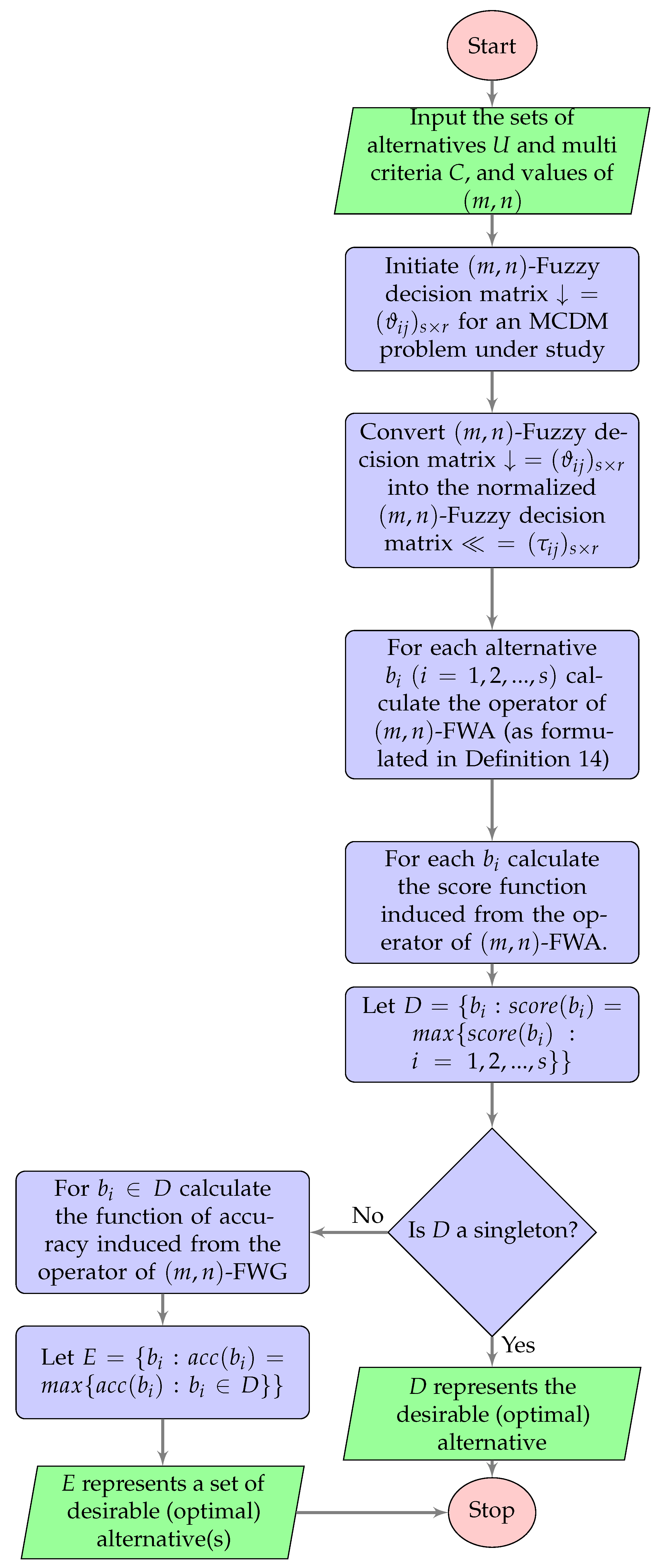
Herein, we give an Algorithm 1 to choose the best alternate using the operator of $(m,n)$-FWA. The algorithms for the other cases of operators are built in a similar way.

The flow chart displayed in Figure 2 shows the way of choosing the optimal alternative(s) via the environment of $(m,n)$-FWA operator. It easy to construct the flow charts of the other operators following a similar way.

Algorithm 1: The optimal alternative(s) induced from the operator of $(m,n)$-FWA.

5.2. Illustrative Examples

We devoted this part to explaining the above-mentioned approaches by the next example.

Example 6. 

A certain company wants to invest a sum of money somewhere. The company management chooses some experts to determine convenient investments out of four potential companies $V=\{$food company, clothes company, computer company, car company}. For this, the experts specify four attributes to evaluate the convenient company as $A=\{a_1=$ growth analysis, $a_2=$ risk analysis, $a_3=$ social-political impact analysis, $a_4=$ annual performance}.

The experts proposed a weight vector corresponding to every criteria $W={(0.2,0.4,0.3,0.1)}^T$. The experts assess the performance of these companies under the $(m,n)$-FSs environment. Assume that the proposed approach for accessing the best company with appreciation to every attribute given by using the experts group is furnished according to the proposed operators for $m=1$ and $n=3$, as follows.

The ordered pairs furnished in

Table 1. $(m,n)$-Fuzzy numbers.

Companies	${\mathit{a}}_1$	${\mathit{a}}_2$	${\mathit{a}}_3$	${\mathit{a}}_4$
food company	(0.8, 0.3)	(0.4, 0.4)	(0.5, 0.7)	(0.2, 0.6)
clothes company	(0.9, 0.4)	(0.4, 0.8)	(0.6, 0.7)	(0.4, 0.7)
computer company	(0.6, 0.5)	(0.5, 0.7)	(0.5, 0.7)	(0.50193, 0.6)
car company	(0.7, 0.6)	(0.2, 0.9)	(0.4, 0.6)	(0.9, 0.1)

describe the degrees given to a company to fulfill (membership) and dissatisfy (non-membership) the corresponding attribute (or criteria).

Now, we apply the proposed operators of aggregation introduced in Definition 14. Then, for each company it computes the score function. If some companies own the same score function, we then must calculate the accuracy functions of them to decide who is the optimal company( or companies); this case is illustrated in the first row of

Table 2. Evaluation of scores with $(1,3)$-Fuzzy aggregation operators.

	Food Company	Clothes Company	Computer Company	Car Company
$(1,3)$-$FWA$	(0.49, 0.49)	(0.56, 0.68)	(0.520193, 0.65)	(0.43, 0.67)
$Score$	0.372351	0.245568	0.245568	0.129237
$Accuracy$	0.607649	0.874432	0.794818	0.730763
$(1,3)$-$FWG$	(0.458391, 0.465150)	(0.531280, 0.660218)	(0.518768, 0.644433)	(0.367683, 0.589892)
$Score$	0.357749	0.243499	0.251139	0.162417
$(1,3)$-$FWPA$	(0.49, 0.1555)	(0.56, 0.3548)	(0.520193, 0.2867)	(0.43, 0.3997)
$Score$	0.48624	0.515337	0.496627	0.366144
$(1,3)$-$FWPG$	(0.591436, 0.550289)	(0.628727, 0.720414)	(0.478361, 0.663311)	(0.489898, 0.780151)
$Score$	0.424799	0.254834	0.186516	−0.015070

.

According to the computations induced from the four operators of aggregation, we find that the optimal ranking order of the four companies induced from a $(1,3)$-$FWA$ operator is a food company. It should be noted that the companies of clothes and computer are equal with respect to the score function; so that we complete comparatione by computing their accuracy functions which show that clothes company is better than computer company to investment. The rank of the candidates induced from a $(1,3)$-$FWA$ operator is

$$\mathrm{food}\mathrm{company}\succ \mathrm{clothes}\mathrm{company}\succ \mathrm{computer}\mathrm{company}\succ \mathrm{car}\mathrm{company}$$

On the other hand, note that the values of score functions induced from the other aggregation operators are distinct for all companies, so there is no need to compute the accuracy function. Thus, the rank of the four companies, respectively, induced from $(1,3)$-$FWG$, $(1,3)$-$FWPA$ and $(1,3)$-$FWPG$ operators are

$$\mathrm{food}\mathrm{company}\succ \mathrm{computer}\mathrm{company}\succ \mathrm{clothes}\mathrm{company}\succ \mathrm{car}\mathrm{company}$$

$$\mathrm{computer}\mathrm{company}\succ \mathrm{clothes}\mathrm{company}\succ \mathrm{food}\mathrm{company}\succ \mathrm{car}\mathrm{company}$$

$$\mathrm{food}\mathrm{company}\succ \mathrm{clothes}\mathrm{company}\succ \mathrm{computer}\mathrm{company}\succ \mathrm{car}\mathrm{company}$$

From the above, it can be noted that the selection of the optimal company is based on two factors, first one is the type of $(m,n)$-FSs, which are estimated by the system experts. The second one is the aggregation operator applied to evaluate the companies.

Remark 3. 

According to the given illustrative example, one can note the following:

(i) 

It cannot be handled the ordered pairs of data given in the illustrative example using IFSs because the sum of the degrees of non-membership and membership is greater than one.

(ii) 

The company management proposed different importances for the degrees of membership and non-membership, which cannot be treated using the extensions of IFSs known in the published manuscripts.

6. Conclusions and Future Works

The vagueness of information is one of the inevitable characteristics of coping with decision-making issues. This vagueness usually originates from the expressions and opinions of decision-makers. It can be defined and captured the uncertainty of information in different approaches; one of them is the fuzzy set theory. In fact, it is a prevailing instrument to deal with uncertainty in decision-making problems. After presenting the fuzzy set theory, it has been developed to different types of orthopairs fuzzy sets such as intuitionistic fuzzy set, Pythagorean fuzzy set, and Fermatean fuzzy sets. It is well known that the orthopairs fuzzy sets represent a simple description of bipolar data, which are the basis of many representation knowledge and reasoning tools.

Herein, we have here presented a new type of orthopair fuzzy sets called $(m,n)$-Fuzzy sets and revealed its connections with other kinds of orthopair fuzzy sets. Two of the merits of $(m,n)$-Fuzzy sets are to, first, expand the grades of membership and non-membership more than IFSs in a way that enables us to cover more situations than IFSs. That is, make us in a position to cope with the information data in which the sum of their grades of membership and nonmembership grades is greater than one. Second, to create appropriate environments to address numerous kinds of real-life problems that cannot be evaluated under the same ranks of importance for the membership and non-membership grades.

On the other hand, the different importance given for the grades of membership and non-membership is a new task for the evaluation process induced from the proposed approach which does not exist in the foregoing generalizations of IFSs. In fact, it needs a comprehensive realization of the situation under study by the experts authorized to evaluate the system inputs.

Through this paper, we have familiarized some operations for $(m,n)$-Fuzzy sets and characterized them. Then, aggregation operators method, as a widely used and popular method in soft computing, have been extended to be used with $(m,n)$-FSs. In the end, these aggregation operators have been employed to diagnosis and analysis decision-making issues. An interpretative example has been provided to illustrate how the proposed approach assisted us with being effective in decision problems than cannot be coped with by the previous classes of IFSs.

Our roadmap for future works is to discuss some applications of $(m,n)$-FSs environment to different fields using (1) the technique for order preference by the similarity to ideal solution, and (2) the weighted aggregated sum product assessment. Additionally, the interaction of $(m,n)$-FSs and rough approximations will be another goal for our future studies. Moreover, we will produce new structures of fuzzy topologies with respect to $(m,n)$-FSs.

References

- Zadeh, L.A. Fuzzy sets. Inf. Control 1965, 8, 338–353. [Google Scholar] [CrossRef] [Green Version]
- Atanassov, K.T. Intuitionistic fuzzy sets. Fuzzy Sets Syst. 1986, 20, 87–96. [Google Scholar] [CrossRef]
- Yager, R.R. Pythagorean membership grades in multicriteria decision making. IEEE Trans. Fuzzy Syst. 2013, 22, 958–965. [Google Scholar] [CrossRef]
- Senapati, T.; Yager, R.R. Fermatean fuzzy weighted averaging/geometric operators and its application in multi-criteria decision-making methods. Eng. Appl. Artif. Intell. 2019, 85, 112–121. [Google Scholar] [CrossRef]
- Kirişci, M.; Demir, I.; Simsek, N. Fermatean fuzzy ELECTRE multi-criteria group decision-making and most suitable biomedical material selection. Artif. Intell. Med. 2022, 127, 102278. [Google Scholar] [CrossRef] [PubMed]
- Yager, R.R. Generalized orthopair fuzzy sets. IEEE Trans. Fuzzy Syst. 2017, 25, 1222–1230. [Google Scholar] [CrossRef]
- Ibrahim, H.Z.; Al-shami, T.M.; Elbarbary, O.G. (3,2)-Fuzzy sets and their applications to topology and optimal choices. Comput. Intell. Neurosci. 2021, 2021, 1272266. [Google Scholar] [CrossRef]
- Al-shami, T.M. (2,1)-Fuzzy sets: Properties, weighted aggregated operators and their applications to multi-criteria decision-making methods. Complex Intell. Syst. 2022, 1–19. [Google Scholar] [CrossRef]
- Al-shami, T.M.; Ibrahim, H.Z.; Azzam, A.A.; L-Maghrabi, A.I.E. SR-fuzzy sets and their applications to weighted aggregated operators in decision-making. J. Funct. Spaces 2022, 2022, 3653225. [Google Scholar] [CrossRef]
- Gao, S.; Zhang, X. Linear orthopair fuzzy sets. Int. J. Fuzzy Syst. 2022, 24, 1814–1838. [Google Scholar] [CrossRef]
- Xu, Z. Intuitionistic fuzzy aggregation operators. IEEE Trans. Fuzzy Syst. 2007, 15, 1179–1187. [Google Scholar]
- Xu, Z.; Yager, R.R. Some geometric aggregation operators based on intuitionistic fuzzy sets. Int. J. Gen. Syst. 2006, 35, 417–433. [Google Scholar] [CrossRef]
- Khan, A.A.; Ashraf, S.; Abdullah, S.; Qiyas, M.; Luo, J.; Khan, S.U. Pythagorean fuzzy dombi aggregation operators and their application in decision support system. Symmetry 2019, 11, 383. [Google Scholar] [CrossRef] [Green Version]
- Peng, X.; Yuan, H. Fundamental properties of Pythagorean fuzzy aggregation operators. Fundam. Informaticae 2016, 147, 415–446. [Google Scholar] [CrossRef]
- Jana, C.; Garg, H.; Pal, M. Multi-attribute decision making for power Dombi operators under Pythagorean fuzzy information with MABAC method. J. Ambient. Intell. Human Comput. 2022, 1–8. [Google Scholar] [CrossRef]
- Peng, X.; Yang, Y.; Song, J.; Jiang, Y. Pythagorean fuzzy soft set and its application. Comput. Eng. 2015, 41, 224–229. [Google Scholar]
- Rahman, K.; Abdullah, S.; Jamil, M.; Khan, M.Y. Some generalized intuitionistic fuzzy Einstein hybrid aggregation operators and their application to multiple attribute group decision making. Int. J. Fuzzy Syst. 2018, 20, 1567–1575. [Google Scholar] [CrossRef]
- Shahzadi, G.; Akram, M.; Al-Kenani, A. Decision-making approach under pythagorean fuzzy yager weighted operators. Mathematics 2020, 8, 70. [Google Scholar] [CrossRef] [Green Version]
- Yager, R.R.; Abbasov, A.M. Pythagorean membership grades, complex numbers and decision making. Int. J. Intell. Syst. 2013, 28, 436–452. [Google Scholar] [CrossRef]
- Jana, C.; Pal, M.; Liu, P. Multiple attribute dynamic decision making method based on some complex aggregation functions in CQROF setting. Comp. Appl. Math. 2022, 41, 103. [Google Scholar] [CrossRef]
- Maji, P.K.; Biswas, R.; Roy, A.R. Fuzzy soft sets. J. Fuzzy Math. 2001, 9, 589–602. [Google Scholar]
- Ahmad, B.; Kharal, A. On Fuzzy Soft Sets. Adv. Fuzzy Syst. 2009, 2009, 586507. [Google Scholar] [CrossRef] [Green Version]
- Alcantud, J.C.R.; Varela, G.; Santos-Buitrago, B.; Santos-García, G.; Jiménez, M.F. Analysis of survival for lung cancer resections cases with fuzzy and soft set theory in surgical decision making. PLoS ONE 2019, 14, e0218283. [Google Scholar] [CrossRef] [PubMed]
- Cağman, N.; Enginoxgxlu, S.; Çitak, F. Fuzzy soft set theory and its application. Iran. J. Fuzzy Syst. 2011, 8, 137–147. [Google Scholar]
- Xu, Y.-J.; Sun, Y.-K.; Li, D.-F. Intuitionistic Fuzzy Soft Set. In Proceedings of the 2010 2nd International Workshop on Intelligent Systems and Applications, Wuhan, China, 22–23 May 2010; pp. 1–4. [Google Scholar] [CrossRef]
- Sivadas, A.; John, S.J. Fermatean Fuzzy Soft Sets and Its Applications. In Computational Sciences—Modelling, Computing and Soft Computing; CSMCS 2020. Communications in Computer and Information Science; Awasthi, A., John, S.J., Panda, S., Eds.; Springer: Singapore, 2021; Volume 1345. [Google Scholar]
- Hamida, M.T.; Riaz, M.; Afzal, D. Novel MCGDM with q-rung orthopair fuzzy soft sets and TOPSIS approach under q-Rung orthopair fuzzy soft topology. J. Intell. Fuzzy Syst. 2020, 39, 3853–3871. [Google Scholar] [CrossRef]
- Al-shami, T.M.; Alcantud, J.C.R.; Mhemdi, A. New generalization of fuzzy soft sets: (a,b)-Fuzzy soft sets. AIMS Math. 2023, 8, 2995–3025. [Google Scholar] [CrossRef]
- Atef, M.; Ali, M.I.; Al-shami, T.M. Fuzzy soft covering-based multi-granulation fuzzy rough sets and their applications. Comput. Appl. Math. 2021, 40, 115. [Google Scholar] [CrossRef]
- Jan, N.; Mahmood, T.; Zedam, L.; Ali, Z. Multi-valued picture fuzzy soft sets and their applications in group decision-making problems. Soft Comput. 2020, 24, 18857–18879. [Google Scholar] [CrossRef]
- Kirişci, M.; Simsek, N. Decision making method related to pythagorean fuzzy soft sets with infectious diseases application. J. King Saud-Univ.-Comput. Inf. Sci. 2022, 34, 5968–5978. [Google Scholar] [CrossRef]
- Yang, B. Fuzzy covering-based rough set on two different universes and its application. Artif. Intell. Rev. 2022, 55, 4717–4753. [Google Scholar] [CrossRef]
- Yang, B.; Hu, B.Q. Communication between fuzzy information systems using fuzzy covering-based rough sets. Int. J. Approx. Reason. 2018, 103, 414–436. [Google Scholar] [CrossRef]
- Ameen, Z.A.; Al-shami, T.M.; Azzam, A.A.; Mhemdi, A. A novel fuzzy structure: Infra-fuzzy topological spaces. J. Funct. Spaces 2022, 2022, 9778069. [Google Scholar] [CrossRef]
- Gulzar, M.; Alghazzawi, D.; Mateen, M.H.; Kausar, N. A Certain Class of t-Intuitionistic Fuzzy Subgroups. IEEE Access 2020, 8, 163260–163268. [Google Scholar] [CrossRef]
- Saleh, S.; Abu-Gdairi, R.; Al-shami, T.M.; Abdo, M.S. On categorical property of fuzzy soft topological spaces. Appl. Math. Inf. Sci. 2022, 16, 635–641. [Google Scholar]
- Senapati, T.; Yager, R.R. Fermatean fuzzy sets. J. Ambient. Intell. Humaniz. Comput. 2020, 11, 663–674. [Google Scholar] [CrossRef]
Figure 1.
Some grade spaces of -FSs.
Figure 2.
Flow chart of selection the optimal alternative(s) with respect to -FWA operator.