A New Nearest Centroid Neighbor Classifier Based on K Local Means Using Harmonic Mean Distance

Abstract

The K-nearest neighbour classifier is very effective and simple non-parametric technique in pattern classification; however, it only considers the distance closeness, but not the geometricalplacement of the k neighbors. Also, its classification performance is highly influenced by the neighborhood size k and existing outliers. In this paper, we propose a new local mean based k-harmonic nearest centroid neighbor (LMKHNCN) classifier in orderto consider both distance-based proximity, as well as spatial distribution of k neighbors. In our method, firstly the k nearest centroid neighbors in each class are found which are used to find k different local mean vectors, and then employed to compute their harmonic mean distance to the query sample. Lastly, the query sample is assigned to the class with minimum harmonic mean distance. The experimental results based on twenty-six real-world datasets shows that the proposed LMKHNCN classifier achieves lower error rates, particularly in small sample-size situations, and that it is less sensitive to parameter k when compared to therelated four KNN-based classifiers.

1. Introduction

KNN [1] is a traditional non-parametric, and most famous, technique among machine learning algorithms [2,3,4]. An instance-based k-nearest-neighbor classifier operates on the premise of first locating the k nearest neighbors in an instance space. Then it uses a majority voting strategy to label the unknown instance with the located nearest neighbors. Due to its simple concept and implementation, its asymptotic classification performance is excellent in Bayes sense, with minimal error rates [5,6]. Also, KNN-based classifiers have a wide range of applications in the field of pattern recognition [7,8], medical imaging [9,10], Electronic Intelligence (ELINT) systems [11], classification and identification of radar signal (i.e., Specific Emitter Identification method—SEI method) [12], fractal analysis [13], SAR technologies, and in the process of construction of database for ELINT/ESM battlefield systems [14], image processing [15],remote sensing [16,17], and biomedical research [18,19,20,21].

Though KNN classification has several benefits, there are still some issues to be resolved. The first matter is that KNN classification performance is affected by existing outliers, especially in small training sample-size situations [22]. This implies that one has to pay attention in selecting a suitable value for neighborhood size k [23]. Firstly, to overcome the influence of outliers, a local mean-based k nearest neighbor (LMKNN) classifier has been introduced in [3]. As LMKNN shows significant performance in response to existing outliers, its concept further applies to distance metric learning [24], group-based classification [6], and discriminant analysis [25]. Pseudo nearest neighbor is another favorable classifier for outliers based on both distance weights as well as local means [26,27]. These classifiers are more robust for existing outliers during classification but are still sensitive to small sample sizes because of noisy and imprecise samples [2,28].

The second matter is finding a suitable distance metric to evaluate the distance between the query sample and training sample, which helps in classification decisions. In order to increase the classification performance of KNN, a number of local and global feature weighting-based distance metrics methods have been developed [29,30]. But these methods ignore the correlation between all training samples; thus, finding an accurate distance metric is considered an important task for KNN classification.

The third matter is that KNN does not consider both properties of a given neighborhood. The concept of neighborhood states (a) neighbors should be as close to query sample as possible, and (b) neighbors should be placed symmetrically around the query sample as possible [24]. The second property is an outcome of the first in the asymptotic cases, but in some practical situations, the geometrical information can become more important than the actual distances incorrectly classifying a query sample [31]. In fact, several alternative neighborhood methods have been successively applied to classification problems, which endeavor to conquer the practical issues in KNN to some extent. For example, the surrounding neighborhood-nearest centroid neighbor (NCN) was successfully derived for finite sample-size situations, and its extensions, KNCN [5] and LMKNCN [4], achieve adequate performance. Despite these methods surpassing KNN classification, there are still some issues, like overestimating the importance of some neighbors, and the assumption that k centroid neighbors have an identical weight, thereby giving rise to unreliable classification decisions [4,5,32,33].

Bearing in mind the superiorities of KNCN and LMKNN, we are motivated to further improve the classification performance of KNN, especially in small sample-size situations. We propose a non-parametric framework for nearest neighbor classification, called A New Nearest Centroid Neighbor Classifier Based on K Local Means Using Harmonic Mean Distance. In our proposed method, the class label with a nearest local centroid-mean vector is assigned to a query sample using the harmonic mean distance as the corresponding similarity measure. The main contributions of LMKHNCN are given below:

• Efficient classification considers not only the distance proximity of k nearest neighbors, but also takes their symmetrical allocation around the query sample into account.
• The proposed framework includes local centroid mean vectors of k nearest neighbors in each class, effectively showing robustness to existing outliers.
• Finally, using Harmonic mean distance as a distance metric, it accounts for more reliable local means in different classes, making the proposed method less sensitive to parameter k.
• Extensive experiments on real world datasets show that our non-parametric framework has better classification accuracy compared to traditional KNN based classifiers.

The rest of this paper is organized as follows. Section 2 briefly summarizes the related work and the motivations for the proposed classifier. In Section 3, we propose a new framework ideology, and show different feature considerations. To verify the proposed method, extensive experiments are conducted to verify the superiority of the proposed method compared to other competitive KNN-based classifiers using twenty-six UCI and KEEL real-world datasets. We present experimental results in Section 4 and draw conclusions in Section 5.

2. Related Work

In this section, we will give a brief review of the KNN-based algorithms used in our framework, and the idea behind the usage of harmonic mean distance as a similarity measure.

2.1. LMKNN Classifier

The KNN classifier is a very famous and simple non-parametric technique in pattern classification. But its classification is easily affected by existing outliers, particularly in small sample-size situations. As an extension of KNN, a local mean-based k nearest neighbor (LMKNN) classifier was developed [3] to overcome the negative effect of outliers. The basic concept of the LMKNN classifier is to compute local mean vectors of k nearest neighbors from each class to classify the query sample. Let $TS={\{p_i\in {ℝ}^d\}}_{i=1}^N$ be a training sample of given d-dimensional feature space, where N is the total number of training samples, and $c_i$ ∈ {$c_1$, $c_2$, …, $c_M$} denotes the class label for $p_i$ with M number of classes. $TR={\{p_{ij}\in {ℝ}^d\}}_{j=1}^{N_i}$ denotes a subset in TS from the class $c_i$ with the number of the training samples $N_i$. LMKNN uses following the steps to classify a query sample $x\in {ℝ}^d$ to class c:

Step 1.

Search the k nearest neighbors from the set TR of each class $c_i$ for the query pattern x. Let $T{R}_k^{NN}\left(x\right)={\{p_{ij}^{NN}\in {ℝ}^d\}}_{j=1}^k$ be the set of KNNs for x in the class $c_i$ using the Euclidean distance metric $d\left(x,p_{ij}^{NN}\right)$, where $k\le N_i$.

$$d\left(x,p_{ij}^{NN}\right)=\sqrt{{(x,p_{ij}^{NN})}^{\mathrm{T}}(x,p_{ij}^{NN})}$$

(1)

Step 2.

Calculate the local mean vector $l{m}_{ik}^{NN}$ from the class $c_i$, using the set $T{R}_k^{NN}\left(x\right)$.

$$l{m}_{ik}^{NN}=\frac{1}{k}{\displaystyle \sum }_{j=1}^K{p}_{ij}^{NN}$$

(2)

Step 3.

Assign x to class c if the distance between the local mean vector for c and the query sample in Euclidean space is minimum.

$$c=\arg \underset{c_i}{\min }d\left(x,l{m}_{ik}^{NN}\right)$$

(3)

Note that the LMKNN is the same as the 1-NN classifier when k = 1. The meaning of K is totally different in LMKNN than KNN. KNN chooses k nearest neighbors from whole training samples, whereas LMKNN uses local mean vector of k nearest neighbors in each class. LMKNN aims at finding the class with the closest local region to the query sample. Therefore, using local mean vectors effectively overcomes the negative effect of outliers, especially in small sample sizes.

2.2. Harmonic Mean Distance

A distance metric is the distance function used to compute the distance between query samples and k nearest neighbors, which helps in classification decisions. The classification performance of the KNN-based classifiers relies heavily on the distance metric used [34,35,36,37,38]. The conventional distance metric used in KNN-based classification is Euclidean Distance, which assumes the data has a Gaussian isotropic distribution. However, if the neighborhood size k is high, the assumption of isotropic distribution is often inappropriate. Therefore, it is very sensitive to neighborhood size k. Many global and local distances metric learning [28,36] have been proposed to improve the performance of KNN-based classifiers. In addition, a harmonic mean distance metric was introduced in the multi-local means-based k-harmonic nearest neighbor (MLMKHNN) classifier [30]. Its classification performance is less sensitive to parameter k and focuses more on reliable local mean vectors. Due to the performance attained by using harmonic mean distance metric, we employ it in our proposed method.

The basic concept of harmonic mean distance is to take the sum of the harmonic average of the Euclidean distances between one given data point and each data point in another point group. In our proposed classifier, harmonic mean distance is used to compute the distance between query sample and each local centroid mean vector to classify the given query sample. For example, if x is the query sample and $T{R}_k^{NCN}\left(x\right)={\{p_{ij}^{NCN}\in {ℝ}^d\}}_{j=1}^k$ is set of its k nearest centroid neighbors from training sample TS = {$TS={\{p_i\in {ℝ}^d\}}_{i=1}^N$, then the harmonic mean distance HMDS ($x$, ${\{p_{ij}^{NCN}\}}_{j=1}^k$) is computed as:

$$\mathrm{HMDS}(x,{\{p_{ij}^{NCN}\}}_{j=1}^k)=\frac{k}{{{\displaystyle \sum }}_{j=1}^k\frac{1}{d(x,{\{p_{ij}^{NCN}\}}_{j=1}^k)}}$$

(4)

where $d(·)$ is the Euclidian distance between query sample x and its k nearest centroid neighbors and ${\displaystyle \sum }_{j=1}^k\frac{1}{d(x,{\{p_{ij}^{NCN}\}}_{j=1}^k)}$ is the harmonic average of Euclidian distances. Using harmonic mean distances considers neighbors with close distance to query sample.

2.3. KNCN Classifier

KNCN is one of the most famous surrounding nearest centroid neighbor classifier [31]. Unlike KNN, KNCN classification considers both distance proximity and symmetrical placements of the nearest neighbors to the query sample. It has been empirically found that KNCN is an effective method in finite sample-size situations. Let $TS={\{p_i\in {ℝ}^d\}}_{i=1}^N$ be a training sample and $c_i$ ∈ {$c_1$, $c_2$, …, $c_M$} denotes the class label for $p_i$ with M number of classes. The centroid of a given set of points $Z=\left(z_1,z_2,\dots ,z_q\right)$ can be calculated:

$$Z_q^c=\frac{1}{q}{\displaystyle \sum }_{i=1}^q{Z}_i$$

(5)

For a given query sample x, its unknown class c can be predicted by KNCN using the steps below:

Step 1.

Search k-nearest centroid neighbors of x from TS using NCN concept,

$$T{R}_k^{NCN}\left(x\right)={\{p_{ij}^{NCN}\in {ℝ}^d\}}_{j=1}^k$$

(6)

Step 2.

Assign x to the class c, which is most frequently represented by the centroid neighbors in the set $T{R}_k^{NCN}\left(X\right)$ (resolve ties randomly).

$$c={\mathrm{argmax}}_{c_j}{{\displaystyle \sum }}_{p_{ij}^{NCN}\in T{R}_k^{NCN}\left(x\right)}\delta \left(c_j=c_n^{NCN}\right)$$

(7)

where $c_n^{NCN}$ is the class label for the nth centroid neighbor $p_{in}^{NCN}$, and δ(cj = $c_n^{NCN}$), the Kronecker delta function, takes a value of one if $c_j=c_n^{NCN}$= , and zero otherwise.

3. The Proposed LMKHNCN Method

3.1. Motivation of LMKHNCN

KNN based classifiers have issues of sensitivity to neighborhood size k, especially in small sample-size situations, which usually have outliers. In the LMKNN classifier, Mitani and Hamamoto have tried to overcome the problem of existing outliers by introducing local mean vectors in each class. These local mean vectors depend heavily upon the neighborhood size k that shows their own class. Even though LMKNN overcomes the outliers problem, its classification performance is more sensitive to the value of neighborhood size k. If the value of k employed is fixed for each class, it may lead to high sensitivity of local mean vectors to the value of k. Also, smallervalues of k providein sufficient classification information, as well as largerk values; can easily takes the outliers in the k nearest neighbors. On the other hand, for uniform k values, it ignores the difference of local sample distribution in different classes and tends to misclassify.

Additionally, according to the concept of neighborhood, nearest neighbors should follow distance-based closeness, and consider spatial distribution in the training set. But KNN-based classifiers only consider distance-based proximity, while in some practical situations, spatial proximity is also important. Thus, to completely follow the concept of neighborhood, a nearest centroid neighbor NCN has been introduced. Furthermore, a k-nearest centroid neighborhood KNCN classifier tries to consider both distance-based proximity and the geometrical distribution of k neighbors to classify a query sample in their training set. The KNCN method achieves better performance in prototype-based classification. However, although KNCN always outperforms KNN, it still has some issues to be resolved, such as estimations of the importance of some neighbors which are not close to the query sample leading to misclassification. Also, like KNN, KNCN makes the inappropriate assumption that k centroid neighbors which have an identical weight can easily tie votes in making classification decisions.

In view of these issues, we were motivated to propose a new nearest centroid neighbor classifier based on k local means using harmonic mean distance. In our proposed classifier, we integrate the supremacies of LMKNN and KNCN classifiers by employing harmonic mean distance as a similarity measure. Firstly, computing the local centroid mean vectors of the k nearest neighbors in each class uses not only the distance nearness, but also considers the symmetrical distribution of the neighbors. Clearly, the local centroid mean vectors in each class have different distances to query samples and have different levels of importance in classification decisions. In other words, our focus should be on the values of k that can find a closer local subclass for the different values of k in each class. Therefore, we used harmonic mean distance metric as a similarity measure between local centroid mean vectors and query samples. Finally, the query sample is classified with class that has the minimum harmonic distance to the query sample. The proposed method reflects on the local centroid mean vectors for classification, therefore making it more robust to outliers, especially in small sample-size situations. Additionally, harmonic mean distance focuses on more consistent local centroid mean vectors in classification decision; this makes it less sensitive to neighborhood size k. The rationale behind the proposed (LMKHNCN), which is a new version of KNN classifier, is described below.

3.2. Description of LMKHNCN

Let ${TS=\{p_i\in {ℝ}^d\}}_{i=1}^N$ be a training set of a given d-dimensional feature space, where N is the total number of training samples, and $c_i$ ∈ {$c_1$, $c_2$, …, $c_M$} denotes the class label for $p_i$ with M number of classes. TR = { ${TR=\{p_{ij}\in {ℝ}^d\}}_{j=1}^{N_i}$ denotes a subset in TS from the class $c_1$ with the number of the training samples $N_i$. In our proposed LMKHNCN classifier, for a given query sample $x\in {ℝ}^d$, its classification is done by following steps:

Step 1:

Find the set of KNCNs $T{R}_k^{NCN}\left(x\right)$ from the set TS of each class $c_i$ for the query sample x,

$$T{R}_k^{NCN}\left(x\right)={\{p_{ij}^{NCN}\in {ℝ}^d\}}_{j=1}^k$$

(8)

using NCN criterion. Note that the value of $k\le N_i$.

Step 2:

Compute the local centroid mean vector $lc{m}_{ik}^{NCN}$ from each class $c_i$ using the set $T{R}_k^{NCN}\left(x\right)$

$$lc{m}_{ik}^{NCN}=\frac{1}{k}{\displaystyle \sum }_{j=1}^K{p}_{ij}^{NCN}$$

(9)

Step 3:

Calculate the harmonic mean distance HMDS (x, $lc{m}_{ik}^{NCN}$) between x and each local centroid mean vector $u_{ik}^{NCN}$.

$$\mathrm{HMDS}\left(x,lc{m}_{ik}^{NCN}\right)=\frac{k}{{{\displaystyle \sum }}_{i=1}^k\frac{1}{d\left(x,lc{m}_{ik}^{NCN}\right)}}$$

(10)

Step 4:

Classify x to the class c, which has the minimum harmonic mean distance between its local centroid mean vector and the query sample x.

$$c={\mathrm{argmin}}_{c_i}\mathrm{HMDS}\left(x,lc{m}_{ik}^{NCN}\right)$$

(11)

It is to be noted that when k = 1, $u_{ik}^{NCN}$ has only one local centroid mean vector, and a harmonic mean distance which is nearly the same as ED, which degrades to LMKNN. It shows the same classification performance as 1-NN. The proposed LMKHNCN classifier is summarized in Algorithm 1 using pseudo code.

Algorithm 1. The proposed MLM-KHNN classifier.

Input:

x: a query sample, k: the neighborhood size.

${TS=\{p_i\in {ℝ}^d\}}_{i=1}^N$: a training set, N1, …, NM: the number of training samples in TS.

${TR=\{p_{ij}\in {ℝ}^d\}}_{j=1}^{N_i}$: class cj training set with Nj training samples.

M: the number of classes, c1, c2, …, cM: class labels in TS,

$N_1,N_2,\dots ,N_{M}N$: the number of training samples in TS.

Output:

c: the classification result of query sample x.

Procedures:

Step 1: Calculate the distances of training samples in each class ci to x.

for j = 1 to Ni do

$$d\left(x,p_{ij}^{NCN}\right)=\sqrt{{\left(x,p_{ij}^{NCN}\right)}^T\left(x,p_{ij}^{NCN}\right)}$$

end for

Step 2: Find the first nearest centroid neighbor of x in each class ci, say $p_{i1}^{NCN}$

[min_index,min_dist] = min(d(x, pij))

$p_{i1}^{NCN}$ = pmin_index

Set $R_i^{NCN}\left(x\right)$ = {$p_{i1}^{NCN}$ ∈ Rm}

Step 3: Search k nearest centroid neighbors of $x$ except the first one, $T{R}_k^{NCN}\left(x\right)={\{p_{ij}^{NCN}\in {ℝ}^d\}}_{j=1}^k$, in each class ci.

for j = 2 to k do

Set Si(x) = TR − $R_i^{NCN}$(x)

Si(x) = ${\left\{pil\in R^d\right\}}_{l=1}^{Li\left(p\right)}$, Li(x) = length(Si(x))

Compute the sum of the previous j − 1 nearest centroid neighbors.

$su{m}_i^{NCN}\left(x\right)$ = ${\displaystyle \sum }_{r=1}^{j-1}{p}_{ir}^{NCN}$

Calculate the centroids in the set Si for $x$.

for l = 1 to Li(x) do

$p_{il}^c$ = 1/j (pil + $su{m}_i^{NCN}$(x))

$d_{il}^c$(x, $p_{il}^c$) = $\sqrt{(x-p_{il}^c)\mathrm{T}(x-p_{il}^c)}$

end for

Find the jth nearest centroid neighbor.

[min_indexNCN, min_distNCN] = min($d_{il}^c$(x, $p_{il}^c$))

$p_{ij}^{NCN}$ = xmin_indexNCN

Add $p_{ij}^{NCN}$ to the set $R_i^{NCN}$.

end for

Set $T{R}_k^{NCN}\left(x\right)$ = $R_i^{NCN}$(x).

Step 4: Calculate the k-local centroid mean vector $lc{m}_{ik}^{NCN}$ in set $T{R}_k^{NCN}\left(x\right)$ for each class ci.

$lc{m}_{ik}^{NCN}$ = 1/r${\displaystyle \sum }_{j=1}^r{p}_{ij}^{NCN}$

Step 5: Compute the harmonic mean distance HMDS(x,$lc{m}_{ik}^{NCN}$) between $x$ and local centroid mean vector $lc{m}_{ik}^{NCN}$ for each class ci,

for j = 1 to M do

HMD(x, $lc{m}_{ik}^{NCN}$) = k/${\displaystyle \sum }_{r=1}^{k}1$/d(x, $lc{m}_{ik}^{NCN}$)

end for

Step 6: Assign $x$ to the class c with a minimum harmonic mean distance.

c = argminciHMDS(x, $lc{m}_{ik}^{NCN}$)

3.3. Comparison with Traditional KNN Based Classifiers

To intuitively explain the distinction of the proposed LMKHNCN method from four state-of-the-art methods (KNN, KNCN, LMKNN and LMKNCN), an informatics comparison is shown in

Table 1. Comparison of KNN, KNCN, LMKNN, LMKNCN, and LMKHNCN classifiers in terms of different feature considerations. The symbols ‘√’and ‘×’, respectively indicate the presence and absence of different features.

Classifier	Distance Proximity	Spatial Distribution	Local Mean Used	Type of Nearest Neighbors	Distance Similarity
KNN	√	×	×	NN	E D
KNCN	√	√	×	NCN	E D
LMKNN	√	×	Local mean of NNs	NN	E D
LMKNCN	√	√	Local mean of NCNs	NCN	E D
LMKHNCN	√	√	Local mean of NCNs	NCN	H M D

. Comparisons are stated based on considerations while computing nearest neighbors, local means, type of nearest neighbors, and distance similarity used. KNN used only distance proximity to find nearest neighbors and Euclidean distance for classification. KNCN considered both distance nearness as well as geometrical allocation while allocating nearest centroid neighbors and classifiers, using ED as a similarity measure. LMKNN is the same as KNN, although it uses Local means of nearest neighbors. LMKNCN combines both KNCN and LMKNN, using Euclidean distance to given weights to local centroid mean vectors. Hence, to reduce sensitivity to k and make it more robust to outliers, LMKHNCN considers both distance proximity as well as symmetrical distribution to classify a query sample into the class of a local centroid mean vector which has the minimum harmonic mean distance to the query sample.

4. Experiment Results and Discussion

In this section we first describe the evaluation metrics and datasets used. Next, we briefly describe the experimental procedure and analyze the various results.

4.1. Performance Evaluation

To authenticate the classification behavior of the proposed classifier in depth, we conduct sets of experiments on twenty-six real data sets and compare the results of the proposed LMKHNCN classifier with the standard KNN classifier and state-of-the-art classifiers. As mentioned in [39], predictions were classified into four groups: true positive $\left(TP\right)$ i.e., when classifier correctly identified the class of the query sample, similarly false positive $\left(FP\right)$ i.e., incorrectly identified, true negative $\left(TN\right)$ i.e., correctly rejected and false negative $\left(FN\right)$ i.e., incorrectly rejected. The classification performance is evaluated by considering the following three metrics: the lowest error rate and the corresponding value of k, sensitivity to the neighborhood size k, and distance between local (centroid) mean vector and query sample.

In pattern classification, the error rate is one of the most effective measures to estimate the performance of algorithms. The error rate of the data distribution is the probability that an instance is misclassified by a classifier that knows the true class probabilities, given the predictors. For a multi classifier, the error rate can be calculated as follows:

$$Errorrate=1-\frac{TP+TN}{TP+TN+FP+FN}$$

(12)

To better evaluate the sensitivity of the proposed classifier to the neighborhood size k, comparative experiments of the classification performance with varying neighborhood size k are also conducted. Sensitivity in terms of predictors is calculated as:

$$Sensitivity=\frac{TP}{TP+FN}$$

(13)

The distance metric used strongly influenced the classification performance of the KNN-based classifiers. Classification is done with minimum distance between local mean vectors and query samples. In our proposed method, minimum harmonic mean distance (HMD) is used to classify the query sample, which can be calculated from Equation (4).

4.2. Description of the Datasets

Twenty-six real-world datasets are taken from the KEEL [40] and UCI machine-learning repositories [41], which are databases concerning diabetic, hill valley, ilpd, plrx, phoneme, sonar, transfusion, bank note, cardiography, sensor, qualitative, winequalityred, steel plates, forest types, balance scale, bands, seeds, vehicle, wine, glass, mice, wdbc, thyroid, and ring. They hold quite different characteristics in terms of number of features, instances, and classes, as described in Table 1. Among twenty-six real-world datasets, there are nine with two-classes; the others are multiclass classification tasks. To comprehensively validate the proposed method, we choose datasets with sample sizes characterized by a wide range, i.e., varying from 182 to 7400. Our goal is to tackle problems with small training sample-size situations, so we randomly selected a training set from each dataset that contained approximately 30% of the data. The rest were chosen as testing data, as shown in

Table 2. Dataset description of twenty-six real-world datasets from UCI and KEEL repository.

DATASET	SAMPLES	ATTRIBUTES	CLASSES	TESTING SET
DIABTIC	1151	20	2	68
HILL VALLEY	1212	101	2	150
ILPD	583	10	2	69
PLRX	182	13	2	65
WPBC	198	32	2	58
TRANSFUSION	748	5	2	155
BANK NOTE	1372	5	2	3315
CARDIOCOGRAPHY 10	2126	22	10	176
THYROID	7200	22	3	2400
SENSOR	5456	5	4	26
QUALITATIVE BANKKRUPTCY	250	7	3	60
WDBC	569	31	2	169
PHONEME	5406	6	2	60
SONAR	208	60	2	66
WINEQUALITYRED	1599	12	4	76
STEEL PLATES	1941	28	7	65
FOREST TYPES	523	28	4	112
BALANCE SCALE	625	5	3	96
RING	7400	21	2	125
BANDS	365	20	2	78
SEEDS	210	8	3	99
VEHICLE1812	846	18	4	282
WINE	178	14	3	59
GLASS	214	11	2	53
MICE	1080	72	8	117

.

4.3. Experimental Procedure

As mentioned earlier, twenty-six real-world datasets are used for our experiments. The environment for the experiments is MATLAB version 8.3.0.532 (R2014a) on intel^® Core™ i5-6500 CPU @3.2 GHz, DELL machine with 4.0 GB RAM. For effective performance, experiments are repeated 10 times, and we obtain 10 different training-test sample sets through 10-fold cross-validation technique in terms of error rate. To establish the superiority of the proposed classifier, its performance is compared to KNN, and its state-of-the-art variants such as KNCN, LMNN and LMKNCN. The value of neighborhood size k is preset in the interval of step size 1, ranging from 1 to 15, and the optimal value on each dataset that corresponds to lowest error rate is considered within that interval. The final outcome is achieved by averaging ten classification error rates with 95% confidence; the best results are in boldface in

Table 3. The lowest error rates (%) of each classifier with the corresponding standard deviation and values of k on twenty-six real-world data sets (the best outcome is marked in bold-face on each data set).

DATASET	KNN		LMKNN		KNCN		LMKNCN		LMKHNCN
DIABTIC	34.08 ± 0.0169	[13]	33.91 ± 0.0158	[14]	31.18 ± 0.0256	[10]	30.48 ± 0.0231	[15]	30.32 ± 0.0237	[14]
HILL VALLEY	40.67 ± 0.0193	[1]	39.23 ± 0.0112	[2]	40.67 ± 0.0426	[1]	30.17 ± 0.0270	[9]	25.77 ± 0.0425	[16]
ILPD	29.85 ± 0.0212	[10]	30.36 ± 0.0171	[14]	30.26 ± 0.0199	[16]	29.03 ± 0.0176	[14]	28.77 ± 0.0221	[13]
PLRX	36.75 ± 0.0154	[1]	36.75 ± 0.0237	[1]	36.75 ± 0.0154	[1]	36.75 ± 0.0159	[1]	35 ± 0.0134	[15]
PHONEME	12.08 ± 0.0183	[1]	12.08 ± 0.0112	[1]	12.08 ± 0.0124	[1]	12.08 ± 0.0290	[1]	11.75 ± 0.0137	[2]
SONAR	17.42 ± 0.0606	[1]	16.36 ± 0.0170	[2]	16.97 ± 0.0398	[7]	14.7 ± 0.0255	[4]	12.88 ± 0.0123	[4]
TRANSFUSION	22.69 ± 0.0137	[7]	23.38 ± 0.0095	[4]	22.15 ± 0.0140	[15]	22.15 ± 0.0119	[12]	21.54 ± 0.0144	[16]
BANK NOTE	0.25 ± 0.0038	[1]	0.20 ± 0.0029	[2]	0.13 ± 0.0029	[3]	0.0009 ± 0.0008	[2]	0.0001 ±0.0008	[4]
CARDIOCOGRAPHY	29.13 ± 0.092	[1]	29.12 ± 0.0124	[1]	27.55 ± 0.0048	[11]	26.95 ± 0.0183	[3]	23.28 ± 0.0152	[5]
THYROID	7.44 ± 0.0123	[12]	7.53 ± 0.0105	[16]	7.24 ± 0.0130	[9]	7.30 ± 0.0098	[5]	7.38 ± 0.0097	[13]
SENSOR	3.22 ± 0.0100	[1]	3.22 ± 0.0072	[1]	2.99 ± 0.0012	[5]	2.7 ± 0.0021	[5]	2.34 ± 0.0022	[7]
QUALITATIVE	0.33 ± 0.0030	[3]	0.33 ± 0.0023	[2]	0.33 ± 0.0028	[5]	0.33 ± 0.0023	[3]	0.33 ± 0.0023	[5]
WINEQUALITYRED	40.8 ± 0.0209	[1]	40.8 ± 0.01169	[1]	40.8 ± 0.0127	[1]	40.8 ± 0.0134	[1]	35.39 ± 0.0161	[15]
WDBC	5.81 ± 0.0075	[10]	5.81 ± 0.0080	[3]	5.13 ± 0.0117	[14]	4.75 ± 0.0076	[16]	5.0 ± 0.0076	[5]
STEEL PLATES	50.66 ± 0.0353	[13]	54.07 ± 0.0151	[10]	49.92 ± 0.0378	[16]	52.66 ± 0.0207	[15]	47.43 ± 0.0376	[16]
FOREST TYPES	10.06 ± 0.0074	[4]	9.45 ± 0.0090	[8]	9.5 ± 0.0099	[11]	9.28 ± 0.0073	[10]	9.06 ± 0.0076	[16]
BALANCE SCALE	15.06 ± 0.0711	[16]	10.94 ± 0.0684	[10]	11.89 ± 0.0858	[16]	9.94 ± 0.0682	[4]	9.06 ± 0.0719	[16]
RING	26.32 ± 0.0623	[1]	10.23 ± 0.0783	[3]	5.39 ± 0.1063	[4]	7.94 ± 0.0740	[2]	7.58 ± 0.0809	[3]
BANDS	34.08 ± 0.0247	[1]	33.68 ± 0.0276	[2]	34.08 ± 0.0221	[1]	34.08 ± 0.0117	[1]	31.2 ± 0.0083	[2]
SEEDS	7.07 ± 0.0071	[1]	6.59 ± 0.0101	[2]	6.83 ± 0.0058	[15]	6.83 ± 0.0113	[3]	5.61 ± 0.0126	[4]
VEHICLE1812	36.11 ± 0.0189	[1]	33..39 ± 0.0189	[2]	31.97 ± 0.0132	[10]	31.24 ± 0.0181	[3]	31.11 ± 0.0119	[12]
Wine	27.29 ± 0.0150	[1]	25.42 ± 0.0101	[9]	22.71 ± 0.0196	[14]	21.02 ± 0.0191	[11]	19.49 ± 0.0224	[16]
WPBC1	29.31±0.0164	[12]	31.55 ± 0.0084	[7]	29.14 ± 0.0166	[11]	28.28 ± 0.0160	[9]	28.45 ± 0.0162	[11]
GLASS	20.56 ± 0.0307	[1]	18.32 ± 0.0197	[2]	20.56 ± 0.0161	[1]	19.72 ± 0.0141	[2]	17.78 ± 0.0131	[3]
MICE	3.72 ± 0.0638	[1]	3.58 ± 0.01380	[2]	3.72 ± 0.0080	[1]	3.25 ± 0.0312	[2]	3 ± 0.0041	[3]

. Thus, to analyze the experimental results on each real-world data set, the lowest error rate with the corresponding standard deviations and values of k is considered as the best outcome, as shown in Table 3.

4.4. Analyzing the Error Rates Results with Corresponding K Value

The experimental comparison results are shown in Table 3, by means of the lowest error rate with the corresponding standard deviations and values of k on each real-world data set. As revealed by the classification results, the proposed LMKHNCN classifier performs better than the other comparative methods in almost all twenty-six real-world data sets. This is because the concept of local centroid mean vector and harmonic mean distance similarity used in the proposed method makes it focus on more reliable local mean vectors with smaller distances to the unknown samples in each class. From the experimental results in Table 3, two interesting facts can be observed: the first is that the error rate of proposed method is somewhat similar to LMKNCN in most dataset cases, because of deploying same concept of integrating KNCN and LMKNN methods; second, the optimal performance of the proposed method is superior to that of KNCN in most cases, which may be attributed to using the local mean vector for each class. Consequently, the proposed classifier is superior to other competitive KNN classifiers.

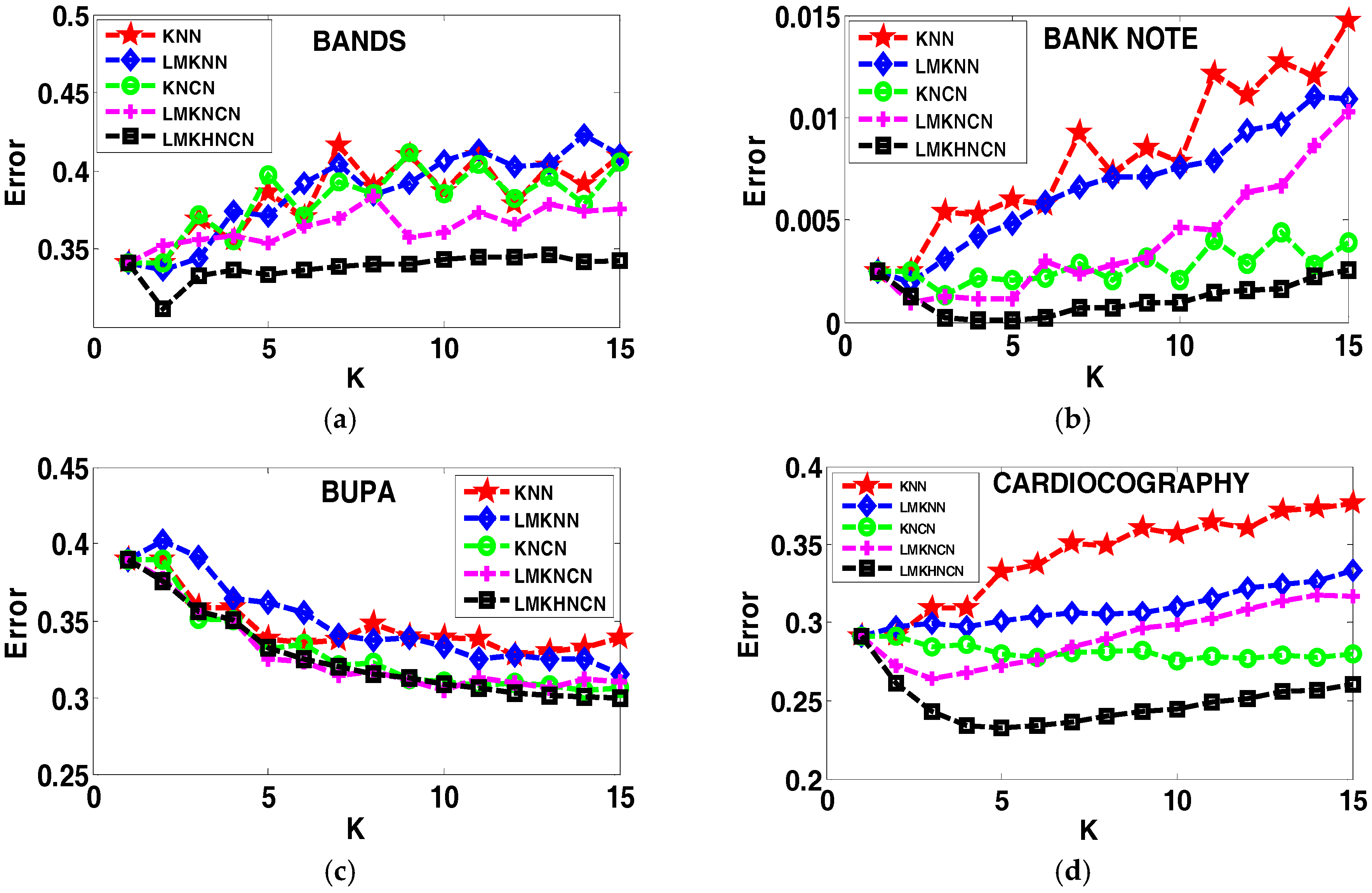
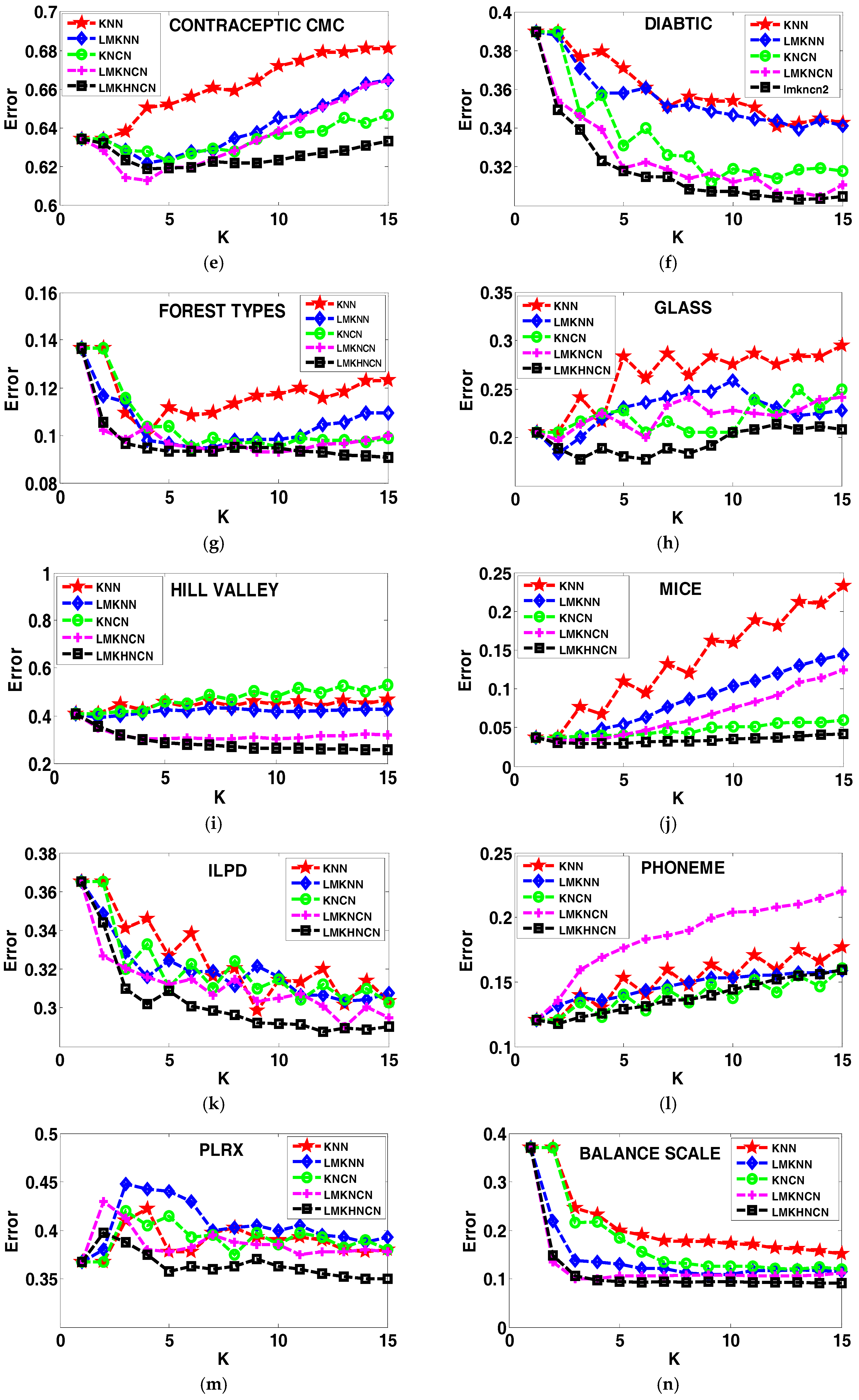
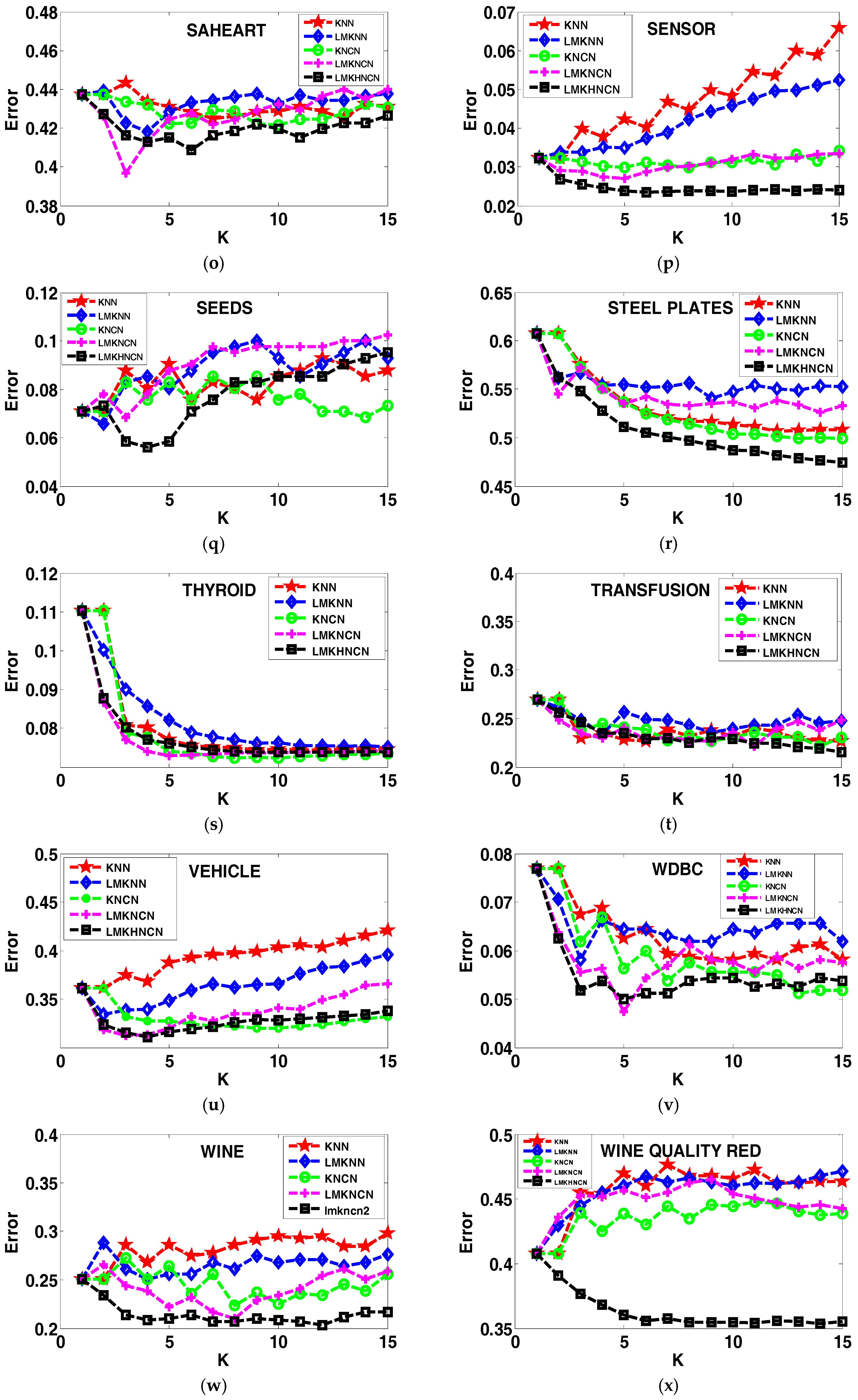
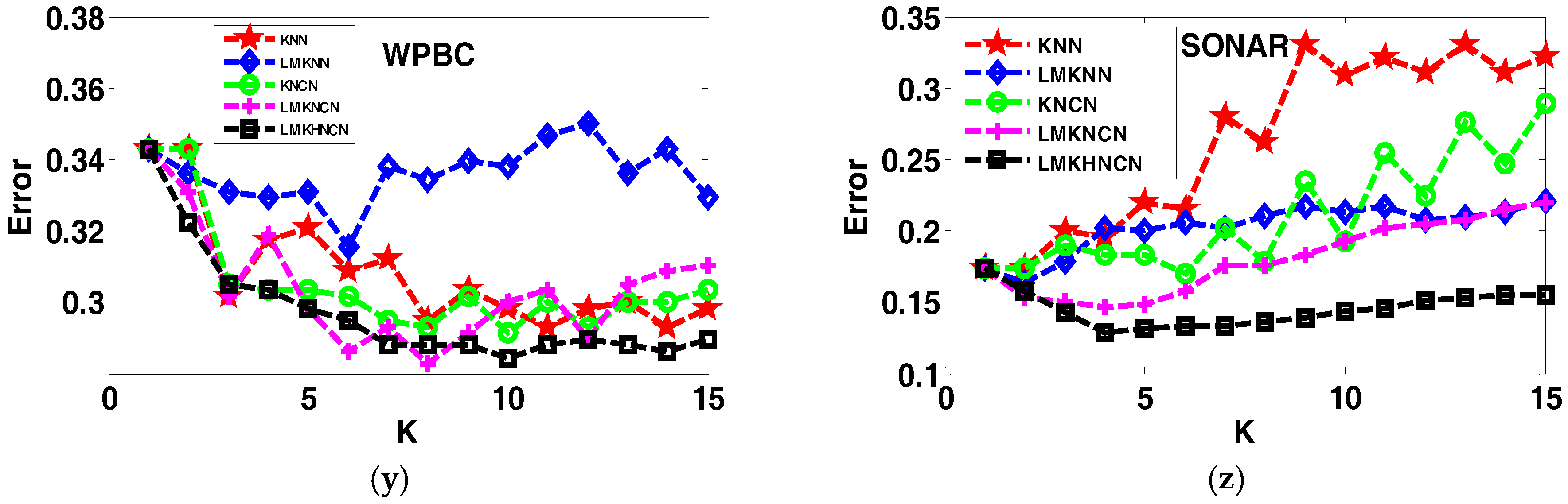
4.5. Results of the Sensitivity to the Neighborhood Size K

To justify the proposed method in terms of sensitivity of the classification performance to the parameter k, experiments have been done on the stated twenty-six real-world datasets in terms of error rates of different classifiers corresponding to neighborhood size k ranging from 1to 15, as shown in Figure 1. From the comparative results, we recognized that the proposed LMKHNCN method has a lower error rate than other classifiers, with different k values for most of the cases. Also, it is detectable that when the value of k is relatively large, the proposed classifier significantly outperforms comparative classifiers. Furthermore, from the graph outcomes, we can observe that the classification error rates of LMKNCN vary with smaller k values of k but become almost stable with larger k values in most cases. But in the case of KNN and LMKNN, it almost continues to increase when values of k increase, which shows that their classification performance is sensitive to neighborhood size k. This strongly indicates that the proposed LMKHNCN method is more robust compared to other methods in most cases, and that its classification performance is less sensitive to neighborhood size k.

4.6. Analyzing the Effect of Distance on Classification Performance

We have analyzed the distances between a local (centroid) mean vector and a given query sample from Balance Scale data set for different values of k particularly in LMKNN, LMKNCN and LMKHNCN classifiers. The query sample taken from class 3 and different distances results are recorded, as shown in

Table 4. The distances between a query sample and the local (centroid)mean vector of each class for values of k, and the classification results on Balance scale data set (1, 2, 3 denote the class labels and symbols ‘√’and ‘×’, respectively, indicate the right and wrong classification. The smallest distances with a nearest local mean vector for each k value among three classes are in bold-faces).

k	Classifier	Class 1	Class 2	Class 3	Classification Result
1	LMKNN	2.247	1.714	1.000	3	√
	LMKNCN	2.247	1.714	1.000	3	√
	LMKHNCN	2.247	1.714	1.000	3	√
2	LMKNN	2.414	1.091	1.523	2	×
	LMKNCN	2.414	1.054	1.423	2	×
	LMKHNCN	2.202	1.032	0.837	3	√
3	LMKNN	2.941	1.742	1.774	2	×
	LMKNCN	2.941	1.125	2.333	2	×
	LMKHNCN	2.854	1.121	1.047	3	√
4	LMKNN	3.173	1.436	1.754	1	×
	LMKNCN	3.112	1.247	0.250	3	√
	LMKHNCN	3.061	1.061	0.000	3	√
5	LMKNN	4.166	1.314	1.846	2	×
	LMKNCN	4.087	1.194	1.283	2	×
	LMKHNCN	4.021	1.020	0.000	3	√

. Classification is done according to the minimum distance between query sample and local (centroid) mean vector. However, from Table 3, it is to be noted that LMKNN and LMKNCN wrongly classified the given query sample when k = 2,3,4,5 and when k = 2,3,5 respectively. As already stated, the query sample does not belong to class 1; thus, the distance difference from class 1 increases as the value of k increases for all classifiers. We have also observed that the local (centroid)mean vector of LMKNN for class 3 becomes more distant from the query sample as k increases, while in LMKHNCN it extends close to the query sample. But in case of LMKHNCN, for k = 1,2,3,4,5, the local (centroid) mean vectors for class 3 are nearer to the query sample than for class 2 with correct classification. Accordingly, the distance results evidently prove the excellence of the proposed LMKHNCN method.

4.7. Analyzing the Computational Complexity

The most important goal for pattern classification is to help attenuate the problem of computation complexities so as to improve the performance of algorithms. In this section, a complexity analysis of online computations in the classification stage for LMKNCN and proposed LMKHNCN classifiers are discussed.

Let $N_{TS}$ denote the number of the training samples, $N_j$ denote the number of training samples in class $c_j$, p the feature dimensionality, M the number of classes, and k the neighborhood size. As mentioned in Section 2.1 for the LMKNN classifier, the classification stage consists of three main steps. The first is to search for the k nearest neighbors in each class based on the Euclidean distance, the multiplications and sum operations are all equal to $O(N_{1}p+N_{2}p+\dots +N_{M}p)$, which can also be abbreviated to $O(N_{TS}p)$. Additionally, the comparisons are $O(N_{1}k+N_{2}k+\dots +N_{M}k)$, which are equal to $O(N_{TS}k)$. The second step is to compute the local mean vector of each class, which requires $O(M_{p}k)$ sum operations. The third and final step assigns the query sample to the class with the smallest distance between its local mean and the given query and is characterized by $O(M_p)$ multiplications and sum operations, whereas the class label is determined with $O\left(M\right)$ comparisons. Thus, the total computational complexity of the LMKNN rule is $O(2N_{TS}p+N_{TS}k+M_{p}k+2M_p+M)$. For the proposed LMKHNCN classifier, its classification stage consists of four steps. The first two steps are almost same as with LMKNCN but using both distance closeness as well as spatial distribution. At the third step, the harmonic mean distance between the query x and each local centroid mean vector is calculated for each class, which requires $O(M_{p}k)$ multiplications and $O(M_{p}k+Mk)$ sum operations, as illustrated in Equation (10). Then, in the final step, the proposed method classifies the query sample to the class with the minimum harmonic mean distance to the given query with $O\left(M\right)$ comparisons. Thus, the total computational complexity of the LMKHNCN rule is $O(2N_{TS}p+N_{TS}k+3M_{p}k+2M_p+Mk+M)$. From the above analysis, it can be seen that the increased computation costs of the proposed method are $O\left(2M_p+Mk\right)>0$. Since the number of classes M and the neighborhood size k are usually much smaller than the value of the training sample size $N_{TS}$, this means that the computational differences are rather small. Therefore, the computational differences between the LMKHNCN classifier and the LMKNN classifier are very small.

5. Conclusions

In this paper, we proposed a new KNN based classifier which allows capturing of classification with local centroid mean vectors by considering the nearness as well as spatial distribution of the k neighbors of each class. It uses the harmonic mean distance as similarity measure, which acknowledges the more reliable local centroid mean vectors that have smaller distances to the query sample. The goal of the proposed method is to overcome the sensitivity of parameter k and reduce the influence of outliers especially in KNCN and LMKNN. To evaluate the performance of the proposed method, extensive experiments on twenty-six real world datasets have been performed in terms of error rate. When compared with KNN, KNCN, LMKNN, and LMKNCN, the proposed method significantly enhances the classification performance, with lower error rates, which demonstrates its robustness to outliers and reduced sensitivity to neighborhood size k. Furthermore, it was shown that when compared with the traditional LMKNN rule, computational differences are very small. In future, we will apply LMKHNCN method to different real-time applications.

References

- Cover, T.; Hart, P. Nearest neighbor pattern classification. IEEE Trans. Inf. Theor. 1967, 13, 21–27. [Google Scholar] [CrossRef] [Green Version]
- Liu, Z.G.; Pan, Q.; Dezert, J. A new belief-based K-nearest neighbor classification method. Pattern Recognit. 2013, 46, 834–844. [Google Scholar] [CrossRef]
- Mitani, Y.; Hamamoto, Y. A local mean-based nonparametric classifier. Pattern Recognit. Lett. 2006, 27, 1151–1159. [Google Scholar] [CrossRef]
- Gou, J.; Yi, Z.; Du, L.; Xiong, T. A local mean-based k-nearest centroid neighbor classifier. Comput. J. 2011, 55, 1058–1071. [Google Scholar] [CrossRef]
- Sánchez, J.S.; Pla, F.; Ferri, F.J. On the use of neighbourhood-based non-parametric classifiers1. Pattern Recognit. Lett. 1997, 18, 1179–1186. [Google Scholar] [CrossRef]
- Samsudin, N.A.; Bradley, A.P. Nearest neighbour group-based classification. Pattern Recognit. 2010, 43, 3458–3467. [Google Scholar] [CrossRef]
- Shanableh, T.; Assaleh, K.; Al-Rousan, M. Spatio-temporal feature-extraction techniques for isolated gesture recognition in Arabic sign language. IEEE Trans. Syst. Man Cybern. Part B 2007, 37, 641–650. [Google Scholar] [CrossRef]
- Xu, J.; Yang, J.; Lai, Z. K-local hyperplane distance nearest neighbor classifier oriented local discriminant analysis. Inf. Sci. 2013, 232, 11–26. [Google Scholar] [CrossRef]
- Maji, P. Fuzzy–rough supervised attribute clustering algorithm and classification of microarray data. IEEE Trans. Syst. Man Cybern. Part B 2011, 41, 222–233. [Google Scholar] [CrossRef] [PubMed]
- Raymer, M.L.; Doom, T.E.; Kuhn, L.A.; Punch, W.F. Knowledge discovery in medical and biological datasets using a hybrid bayes classifier/evolutionary algorithm. IEEE Trans. Syst. Man Cybern. Part B 2003, 33, 802–813. [Google Scholar] [CrossRef] [PubMed]
- Dudczyk, J.; Kawalec, A.; Owczarek, R. An application of iterated function system attractor for specific radar source identification. In Proceedings of the 17th International Conference on Microwaves, Radar and Wireless Communications, Wroclaw, Poland, 19–21 May 2008; pp. 1–4. [Google Scholar]
- Dudczyk, J.; Kawalec, A.; Cyrek, J. Applying the distance and similarity functions to radar signals identification. In Proceedings of the 2008 International Radar Symposium, Wroclaw, Poland, 21–23 May 2008; pp. 1–4. [Google Scholar]
- Dudczyk, J.; Wnuk, M. The utilization of unintentional radiation for identification of the radiation sources. In Proceedings of the 34th European Microwave Conference, Amsterdam, The Netherlands, 12–14 October 2004; pp. 777–780. [Google Scholar]
- Dudczyk, J. A method of feature selection in the aspect of specific identification of radar signals. Bull. Pol. Acad. Sci. Tech. Sci. 2017, 65, 113–119. [Google Scholar] [CrossRef] [Green Version]
- Mensink, T.; Verbeek, J.; Perronnin, F.; Csurka, G. Distance-based image classification: Generalizing to new classes at near-zero cost. IEEE Trans. Pattern Anal. Mach. Intell. 2013, 35, 2624–2637. [Google Scholar] [CrossRef] [PubMed]
- Frigui, H.; Gader, P. Detection and discrimination of land mines in ground-penetrating radar based on edge histogram descriptors and a possibilistic k-nearest neighbor classifier. IEEE Trans. Fuzzy Syst. 2009, 17, 185–199. [Google Scholar] [CrossRef]
- Ma, L.; Crawford, M.M.; Tian, J. Local manifold learning-based k-nearest-neighbor for hyperspectral image classification. IEEE Trans. Geosci. Remote Sens. 2010, 48, 4099–4109. [Google Scholar] [CrossRef]
- Manavalan, B.; Shin, T.H.; Lee, G. PVP-SVM: Sequence-based prediction of phage virion proteins using a support vector machine. Front. Microbiol. 2018. [Google Scholar] [CrossRef] [PubMed]
- Manavalan, B.; Subramaniyam, S.; Shin, T.H.; Kim, M.O. Machine-learning-based prediction of cell-penetrating peptides and their uptake efficiency with improved accuracy. J. Proteome Res. 2018, 17, 2715–2726. [Google Scholar] [CrossRef] [PubMed]
- Manavalan, B.; Shin, T.H.; Lee, G. DHSpred: Support-vector-machine-based human DNase I hypersensitive sites prediction using the optimal features selected by random forest. Oncotarget 2018, 9, 1944–1956. [Google Scholar] [CrossRef] [PubMed]
- Manavalan, B.; Shin, T.H.; Kim, M.O.; Lee, G. AIPpred: Sequence-based prediction of anti-inflammatory peptides using random forest. Front. Pharmacol. 2018, 9, 276. [Google Scholar] [CrossRef] [PubMed]
- Fukunaga, K. Introduction to Statistical Pattern Recognition; Elsevier: Amsterdam, The Netherlands, 2013. [Google Scholar]
- Bhattacharya, G.; Ghosh, K.; Chowdhury, A.S. A probabilistic framework for dynamic k estimation in kNN classifiers with certainty factor. In Proceedings of the 2015 8th International Conference on Advances in Pattern Recognition, Kolkata, India, 4–7 January 2015. [Google Scholar]
- Chai, J.; Liu, H.; Chen, B.; Bao, Z. Large margin nearest local mean classifier. Signal Process. 2010, 90, 236–248. [Google Scholar] [CrossRef]
- Yang, J.; Zhang, L.; Yang, J.Y.; Zhang, D. From classifiers to discriminators: A nearest neighbor rule induced discriminant analysis. Pattern Recognit. 2011, 44, 1387–1402. [Google Scholar] [CrossRef]
- Zeng, Y.; Yang, Y.; Zhao, L. Pseudo nearest neighbor rule for pattern classification. Expert Syst. Appl. 2009, 36, 3587–3595. [Google Scholar] [CrossRef]
- Gou, J.; Zhan, Y.; Rao, Y.; Shen, X.; Wang, X.; He, W. Improved pseudo nearest neighbor classification. Knowl. Based Syst. 2014, 70, 361–375. [Google Scholar] [CrossRef]
- Xu, Y.; Zhu, Q.; Fan, Z.; Qiu, M.; Chen, Y.; Liu, H. Coarse to fine K nearest neighbor classifier. Pattern Recognit. Lett. 2013, 34, 980–986. [Google Scholar] [CrossRef]
- Chen, L.; Guo, G. Nearest neighbor classification of categorical data by attributes weighting. Expert Syst. Appl. 2015, 42, 3142–3149. [Google Scholar] [CrossRef]
- Lin, Y.; Li, J.; Lin, M.; Chen, J. A new nearest neighbor classifier via fusing neighborhood information. Neurocomputing 2014, 143, 164–169. [Google Scholar] [CrossRef]
- Chaudhuri, B.B. A new definition of neighborhood of a point in multi-dimensional space. Pattern Recognit. Lett. 1996, 17, 11–17. [Google Scholar] [CrossRef]
- Grabowski, S. Limiting the set of neighbors for the k-NCN decision rule: Greater speed with preserved classification accuracy. In Proceedings of the International Conference Modern Problems of Radio Engineering, Telecommunications and Computer Science, Lviv-Slavsko, Ukraine, 24–28 Feburary 2004. [Google Scholar]
- Sánchez, J.S.; Pla, F.; Ferri, F.J. Improving the k-NCN classification rule through heuristic modifications. Pattern Recognit. Lett. 1998, 19, 1165–1170. [Google Scholar] [CrossRef] [Green Version]
- Bailey, T.; Jain, A.K. A note on distance-weighted k-nearest neighbor rules. IEEE Trans. Syst. Man Cybern. 1978, 311–313. [Google Scholar] [CrossRef]
- Yu, J.; Tian, Q.; Amores, J.; Sebe, N. Toward robust distance metric analysis for similarity estimation. In Proceedings of the 2006 IEEE Computer Society Conference on Computer Vision and Pattern Recognition (CVPR’06), New York, NY, USA, 17–22 June 2006; pp. 316–322. [Google Scholar]
- Gou, J.; Du, L.; Zhang, Y.; Xiong, T. A new distance-weighted k-nearest neighbor classifier. J. Inf. Comput. Sci. 2012, 9, 1429–1436. [Google Scholar]
- Wang, J.; Neskovic, P.; Cooper, L.N. Improving nearest neighbor rule with a simple adaptive distance measure. Pattern Recognit. Lett. 2007, 28, 207–213. [Google Scholar] [CrossRef]
- Pan, Z.; Wang, Y.; Ku, W. A new k-harmonic nearest neighbor classifier based on the multi-local means. Expert Syst. Appl. 2017, 67, 115–125. [Google Scholar] [CrossRef]
- Manavalan, B.; Shin, T.H.; Kim, M.O.; Lee, G. PIP-el: A new ensemble learning method for improved proinflammatory peptide predictions. Front. Immunol. 2018, 9, 1783. [Google Scholar] [CrossRef] [PubMed]
- Alcalá-Fdez, J.; Fernández, A.; Luengo, J.; Derrac, J.; Garcí, S.; Sánchez, L.; Herrera, F. Keel data-mining software tool: Data set repository, integration of algorithms and experimental analysis framework. J. Mult.-Valued Log. Soft Comput. 2011, 17, 255–287. [Google Scholar]
- Bache, K.; Lichman, M. Uci machine learning repository [http://archive. ics. uci. edu/ml]. irvine, ca: University of california, school of information and computer science. begleiter, h. neurodynamics laboratory. state university of new york health center at brooklyn. ingber, l.(1997). statistical mechanics of neocortical interactions: Canonical momenta indicatros of electroencephalography. Phys. Rev. E 2013, 55, 4578–4593. [Google Scholar]
Figure 1.
The error rates of each classifier corresponding to value of neighborhood size k on twenty-six real world datasets.