MODC: A Pareto-Optimal Optimization Approach for Network Traffic Classification Based on the Divide and Conquer Strategy


Informatics Center, Federal University of Pernambuco, UFPE, Recife-PE 50740-560, Brazil
*
Author to whom correspondence should be addressed.
Information 2018, 9(9), 233; https://0-doi-org.brum.beds.ac.uk/10.3390/info9090233
Submission received: 13 August 2018
/
Revised: 10 September 2018
/
Accepted: 11 September 2018
/
Published: 13 September 2018
(This article belongs to the Section Information and Communications Technology)
Abstract
:Network traffic classification aims to identify categories of traffic or applications of network packets or flows. It is an area that continues to gain attention by researchers due to the necessity of understanding the composition of network traffics, which changes over time, to ensure the network Quality of Service (QoS). Among the different methods of network traffic classification, the payload-based one (DPI) is the most accurate, but presents some drawbacks, such as the inability of classifying encrypted data, the concerns regarding the users’ privacy, the high computational costs, and ambiguity when multiple signatures might match. For that reason, machine learning methods have been proposed to overcome these issues. This work proposes a Multi-Objective Divide and Conquer (MODC) model for network traffic classification, by combining, into a hybrid model, supervised and unsupervised machine learning algorithms, based on the divide and conquer strategy. Additionally, it is a flexible model since it allows network administrators to choose between a set of parameters (pareto-optimal solutions), led by a multi-objective optimization process, by prioritizing flow or byte accuracies. Our method achieved 94.14% of average flow accuracy for the analyzed dataset, outperforming the six DPI-based tools investigated, including two commercial ones, and other machine learning-based methods.
1. Introduction
Network traffic classification aims to identify categories of traffic or applications of network packets or flows. It is an area that continues to gain attention by researchers [1,2,3,4,5,6,7,8,9,10,11,12,13,14,15,16,17]. Due to the growth of the Internet, both in the number of applications and traffic volume, it is important to understand the composition of such data, especially by Internet Service Providers (ISPs) to manage bandwidth resources, with focus on the Quality of Service (QoS) and security.
The “Internet of Things” (IoT) is evolving and might be connecting billions of devices by 2020 [18] and more than $11 trillion by 2025 [19]. Hence, along with the smart cities, issues of cyber security might become greater than ever [7], with organizations possibly not knowing exactly what IoT devices are generating traffic within their networks [20] and which kind of traffic. It is expected that traditional security tools would not handle the processing of such a huge amount of data (i.e., “big data”) and services [7]. This encourages the use of machine learning for network traffic classification and intrusion detection, which can aid in the identification of hidden and unexpected patterns, also for big data (e.g., deep learning [21,22,23,24]), and can also be used to learn and understand the processes that generate the data [25].
There are many methods for classifying network traffic. The most common methods are the classification by using known transport layer ports (port-based methodology) and Deep Packet Inspection (DPI) [14,26,27]. The port-based method analyzes the port numbers from the transport layer and is utilized to classify applications (e.g., Skype, BitTorrent, Edonkey) or application protocols (e.g., HTTP, FTP, DNS, SSH). This method proved to be ineffective since random ports can be used by individual applications. A more effective method is using a DPI technique, which eliminates the problem of random ports. The technique starts by reading payloads from packets and performs scans with the objective of extracting signatures from network traffic data. These signatures can then be used to identify network traffic types. The DPI-based classification method for network traffic is usually considered the most accurate. This is the reason why many commercial solutions rely on it [14]. However, this approach breaks when dealing with encrypted traffic data and when multiple signatures might match. Additionally, the high computational cost makes payload-based methods face performance issues in real world networks [28,29], aside from the concerns about users’ privacy, since DPI relies on packet payloads inspection.
As a result, machine learning has been used for network traffic classification [1,2,4,5,6,7,8,10,11,12,13,17,30,31,32] due to its good generalization capability and the ability to tackle such DPI issues (i.e., encrypted data, performance issues and users’ privacy concerns). This area of research is still in evidence stages [2,3,4,6,25,33] and has shown to be accurate when dealing with applications and application protocols classification.
Although many works have been proposed, the majority of them have not paid enough attention to certain issues, mainly related to experimental procedures. Private datasets are frequently used in the experiments, which prevent researchers from reproducing the results, making it difficult to benchmark network traffic classifiers. Additionally, there is a gap regarding the classification based on byte accuracy. Most studies focus on packet or flow classification accuracies, but usually ignore byte classification accuracy.
Flows are commonly classified as elephant (flows with large byte volume) or mice (flows with small byte volume). Both types are important in network traffic classification, since elephant flows can impact a low bandwidth network and mice flows can contain unwanted traffic data such as malicious software and network policy violations data (e.g., chatting, data uploading with cloud-based software or FTP, and piracy issues). There have been few works [10,34] that analyze the byte accuracy performance measure. Nevertheless, they focus mainly on the flow or packet classification accuracy, presenting byte accuracy results for analysis purposes, but with no intention of simultaneously optimizing both accuracies. Commercial and free classification tools [14] also share a single objective: to reach high rates of traffic classification accuracy. For networks with low bandwidth, very common in less developed countries, for example, it is crucial to correctly classify elephant flows due to the lack of network resources, and that is the reason why the byte accuracy measure should also be the focus. Consequently, there is a need for a classifier that could be flexible enough to let network administrators adjust it according to their needs.
Therefore, this work proposes a hybrid model, composed of machine learning algorithms, which supports this flexibility by optimizing such model with the use of the Multi-Objective Genetic Algorithm (MOGA). Additionally, to cope with the dataset and experimental issues, as mentioned earlier, this work pretends to perform the experiments with a public dataset, containing a large set of applications and application protocols, with the results being compared to six commonly used network traffic classifiers (DPI), including commercial ones. Additionally, a benchmark against other machine learning-based methods is performed. This work can thus allow researchers to compare their methods to the hybrid model being proposed in this work, since comparisons between network traffic classifiers are known for being a difficult task in this area of research [35].
In a nutshell, the proposed hybrid model is composed of supervised and unsupervised machine learning algorithms, in addition to a feature selection process, and is based on the divide and conquer strategy [36]. The dividing process is led by an unsupervised algorithm, the Growing Hierarchical Self-Organizing Map (GHSOM) [37], and focuses on the division of a huge and complex problem into smaller and simpler tasks, that is, into clusters. The conquer process then attacks the less complex tasks (smaller datasets or clusters) using a supervised learning algorithm, the Extreme Learning Machine (ELM) [38]. This strategy proved to enhance the learning process [36] and has never yet been tested in network traffic classification. Additionally, the MOGA algorithm is utilized to optimize all the process. To the best of our knowledge, there have been no contributions that investigate the use of a divide and conquer strategy for network traffic classification, along with the flexibility of allowing network administrators to choose the best parameters for their networks, by prioritizing flow or byte classification accuracy. This can be performed with the use of multi-objective optimization, by selecting between pareto-optimal solutions. Besides that, this work is compared against commonly used network traffic classifiers and machine learning algorithms, the results of which could benefit the benchmarking of different methodologies.
The remainder of the paper is organized as follows. In Section 2, we review the literature on network traffic classification with the aid of machine learning. Section 3 presents the proposed method, and Section 4 shows the experimental settings and results. Finally, Section 5 concludes the paper with future research directions.
2. Literature Review
To overcome the drawbacks of DPI tools, machine learning methods have been proposed to deal with such a complex task, usually by using unsupervised and supervised learning algorithms. Classification algorithms (i.e., supervised) identify category labels of instances which, in most cases, are described by a set of features. Models are generated by training such labeled datasets, usually in a supervised learning process, and infer the class labels for the instances (usually packets or flows) of new network traffic data. The use of such techniques has shown to be highly accurate, even on encrypted traffic [11,39,40,41]. Some works make use of unsupervised learning [42,43,44], mostly for unknown traffic labeling, where instances are grouped by similarity in clusters. In unsupervised learning, there are no explicit target outputs for each input, that is, the dataset used in the training process is unlabeled.
Few studies focus on the use of semi-supervised algorithms. These are commonly used when the cost of labeling instances for the learning process is too high or when the minority of instances in a dataset are labeled, and the remaining are not, which can be easily collected in computer networks. The classifiers proposed by [45,46] were shown to be accurate, presenting results above 90% of flow accuracy by using semi-supervised Support Vector Machine (SVM) and k-means based algorithms, respectively.
Besides the use of supervised and unsupervised learning algorithms, some studies make use of optimization algorithms in order to enhance the quality of their methods [12,16]. Optimization algorithms are usually used to find the best set of parameters aiming to enhance the results, either by minimizing or maximizing a function (e.g., to maximize the flow accuracy metric in network classification problems, where the function is the classifier algorithm (model) itself). Multi-objective optimization has already been used in network traffic classification, but only for feature selection optimization [47] and network anomaly detection [48]. In [49], the optimization occurred during the feature selection and clustering processes only, with no concern with the enhancement, simultaneously, of two important metrics for network administrators, the byte and flow classification accuracies. We propose to address this limitation by developing a flexible hybrid model so that network administrators can choose what needs to be classified, that is, the flow or byte accuracy, according to their network environment needs (there is a trade-off when selecting the best parameter between the pareto-optimal solutions, as will be explained in Section 3).
Our brief literature review demonstrates that different methodologies have been proposed to deal with the difficult task of network traffic classification, including various types of machine learning techniques. Indeed, many works have been proposed, but the majority of them has not paid sufficient attention to the following items:
- Reproducibility is not possible when the dataset used in the experiments is private and, therefore, hinders the benchmarking against different network traffic classifiers.
- The correct labeling (i.e., ground-truth or GT) of flow instances is necessary to build good classifiers.
- Port and IP information should be discarded from network datasets since applications can make use of random ports or the traffic can be encapsulated, and IP information in packets can be obfuscated by proxies.
- Some network administrators would be more concerned to correctly classify flows which require more bandwidth resources from a network; that is, the accuracy of bytes would be more important than the accuracy of flows.
This paper distinguishes itself from others by paying attention to all the issues described above, mainly by proposing a flexible hybrid model, with the aid of a multi-objective optimizer, to make it possible for network administrators to select the best set of parameters according to their needs (i.e., flow or byte accuracy). Additionally, the proposed model is based on the divide and conquer strategy, by combining supervised and unsupervised learning algorithms, which enhances the overall classification accuracy and, to the best of our knowledge, has never yet been attempted on network traffic classification.
3. The Proposed Method
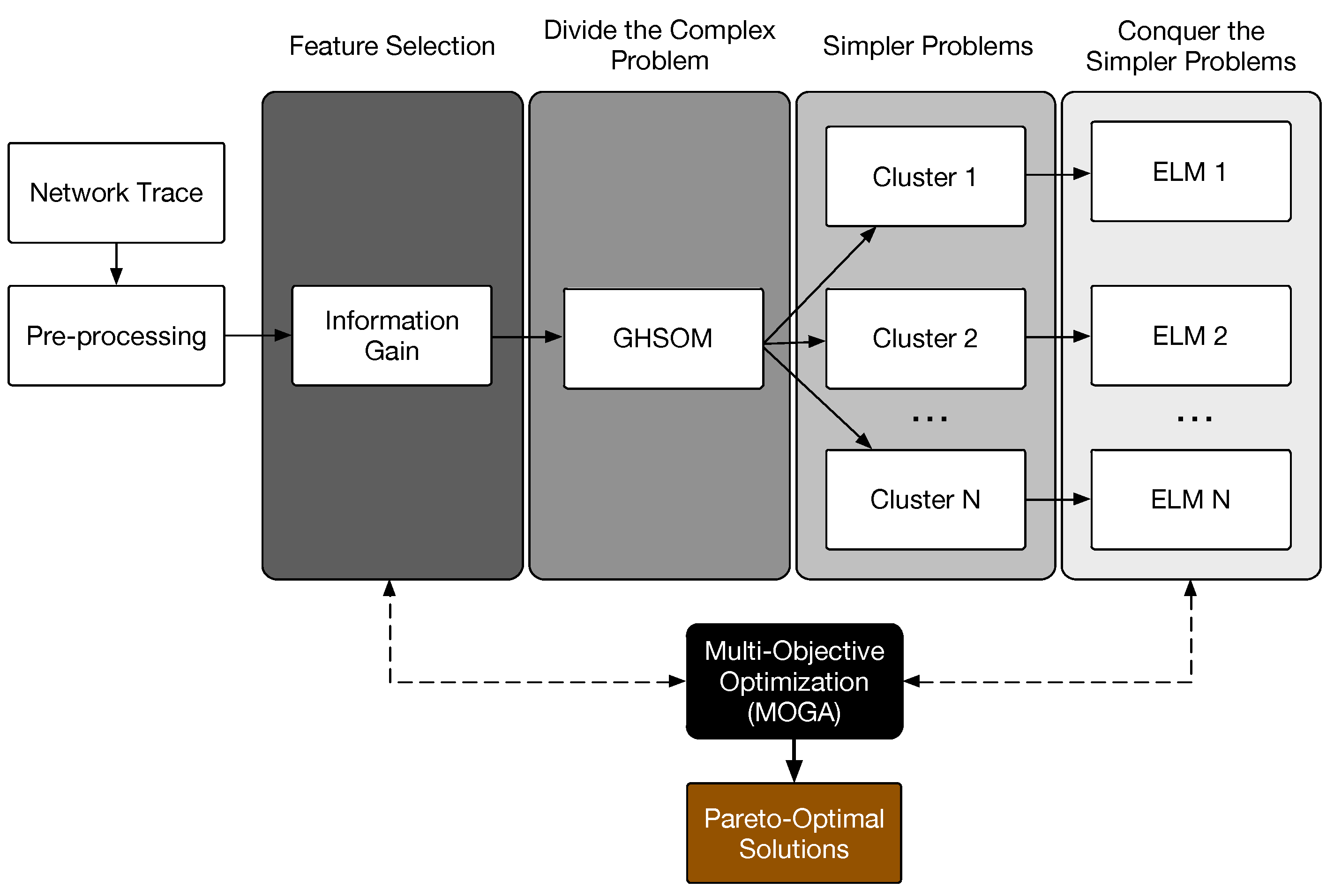
The authors in [36] claim that if a model is trained to perform different subtasks on different occasions, there will generally be strong interference effects that lead to poor generalization and slow learning. On the other hand, the authors also claim that, if a training dataset can be naturally divided into subsets, representing distinct subtasks, interference can be reduced by using different expert models for each subtask. This system also has a gating model that decides which of the experts should be selected for each subtask [36]. In this strategy, known as “divide and conquer”, a complex problem can be divided into simpler subproblems and attacked by individual expert models. Inspired by this strategy, we propose a hybrid model for network traffic classification, named the Multi-Objective Divide and Conquer (MODC) model, where the problem is split into subproblems with the aid of an unsupervised learning model and attacked by individual supervised learning models, where the gating model is the unsupervised learning model itself. As mentioned before, this strategy has never been tested on network traffic classification. Additionally, this hybrid model is optimized by a multi-objective algorithm, turning the model into a flexible solution for network administrators, by prioritizing the accuracy in bytes, flows, or a more balanced selection. The proposed method can be visualized in Figure 1, in which the training process, responsible for generating the complete model (i.e., the network traffic classifier), will be detailed in the following sections.
3.1. Feature Selection
The complete model is created by training the divide and conquer phases, as seen in Figure 1. Nonetheless, before the training phases, selecting a subset of features from the network trace (dataset), instead of using all the available features, can enhance the final model quality. This can be performed by using feature selection algorithms. The network trace and pre-processing boxes in Figure 1 will be further explained in Section 4.
The feature selection consists of choosing one feature (attribute) subset among a complete feature set that maximizes the model quality by filtering unnecessary features. In our methodology, we have used the Information Gain [50] algorithm for being the best one when compared to others in our previous work [41]. The Information Gain is commonly used in decision tree algorithms, but it can also be used for the feature selection purpose. The higher the score obtained by a particular feature, the better it can contribute to enhancing the model quality by producing more accurate classification results.
For the classification task, the Information Gain (IG) measures how common a feature is in a class when compared to all other classes in a particular dataset, by analyzing the presence or absence of a term t. The IG determines how much information a particular attribute, or feature, contributes to the training and classification process. Understandably, features with high information gain are preferred to be used during the training process. A term is a word (category) that might be repeated throughout the dataset, in different attributes. For continuous-valued attributes, it is necessary to transform the dataset into categories, which, in this work, the methodology proposed by [51] was applied to. Let be a set of classes in a training dataset. The information gain of a term t is defined by Equation (1). This includes the a priori probability () of a term t, besides the a posteriori probability of a class given the term t, that is, , and the a priori probability of a class in the training dataset. To obtain the information gain score from a specific feature (attribute), it is necessary to calculate the right-hand side of the sum of Equation (1) for each term t in that feature, sum the obtained values, and then sum the result with the left-hand side of the summation in Equation (1).
3.2. Divide
The dividing phase consists of splitting a complex problem into smaller and simpler ones. The task of generating a classifier model trained with a dataset containing more similar instances (i.e., sharing the same or approximate statistical distribution), by dividing the complete dataset into clusters and then conquering each partition by training an individual supervised learning model for each cluster, has shown to be more efficient than training a single expert (classifier) for the full dataset [36]. Both the divide and conquer phases can be visualized in Figure 1.
The dividing process starts after the feature selection phase and utilizes the Growing Hierarchical Self-Organizing Map (GHSOM) algorithm [37] as the clustering technique. The GHSOM is an unsupervised learning algorithm and is based on the Self-Organizing Map (SOM) algorithm [52]. It has the capability of dynamically modeling the dataset into clusters, without the need of specifying a predefined number of clusters (grid size), in contrast to the SOM algorithm, which requires the grid size input. Thus, for the GHSOM, no prior information of the problem should be known. Additionally, the modeling is refined by a hierarchical growing process, where individual clusters can be extended to new self-organizing maps. This way, the network trace should be split into n clusters, in which n is automatically determined by the GHSOM, where each cluster represents instances more similar to each other, that is, a subtask or a dataset partition.
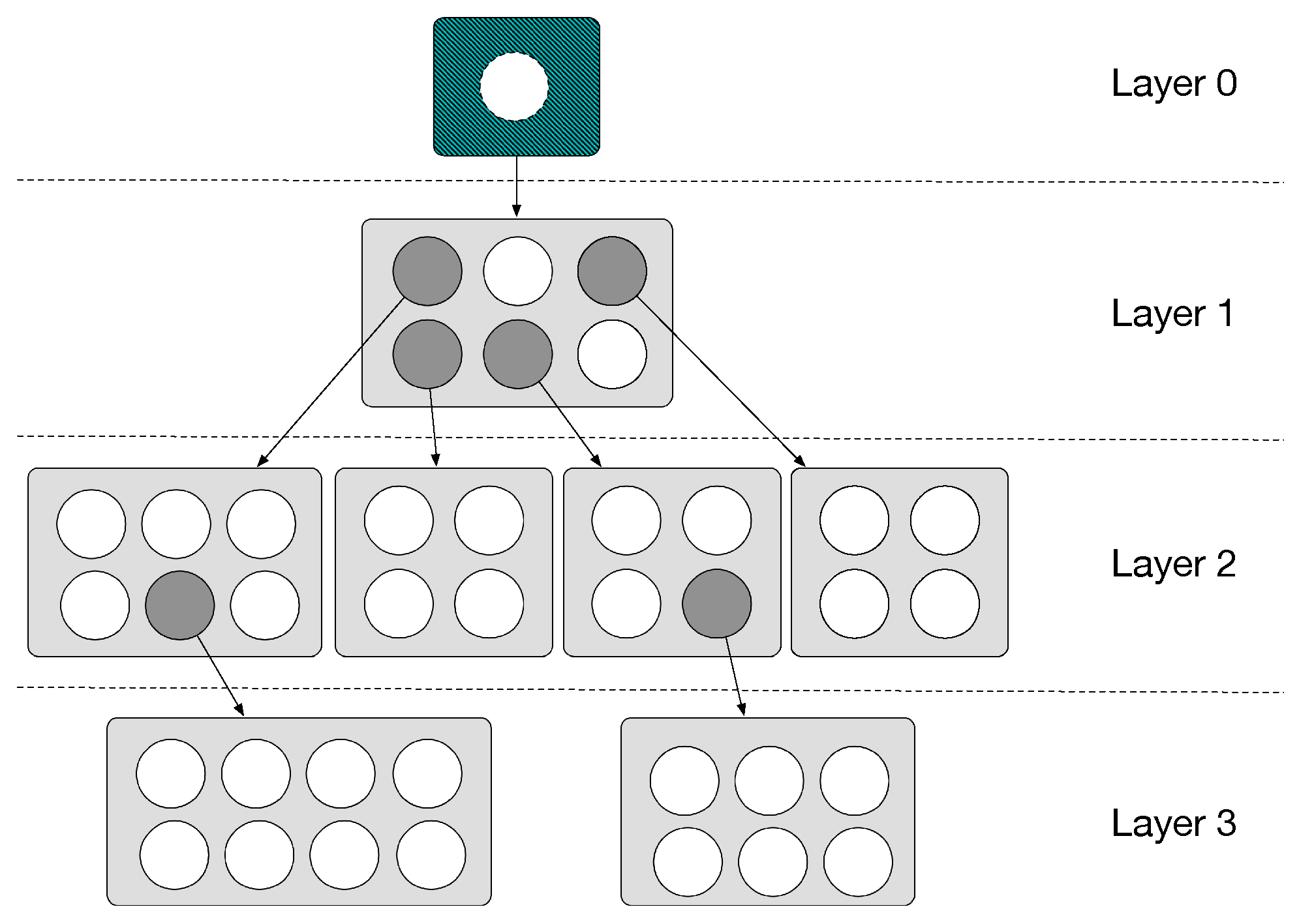
As already mentioned, besides grouping instances by similarity (based on the input space), into clusters, the GHSOM is also capable of creating clusters in a hierarchical way according to the data distribution, by expanding nodes into new layers, as can be visualized in Figure 2. For example, at Layer 0, the complete dataset is available and is divided into clusters at Layer 1. Nodes can then be expanded into new SOM maps (e.g., maps at Layer 2) or can grow in a horizontal way, that is, the size of each map adapts itself based on the input space data. The maps continue to grow, horizontally (i.e., in breadth) and hierarchically (i.e., in depth), building a data structure with many layers consisting of independent Self-Organizing Maps (SOMs).
3.3. Conquer
The conquering phase is responsible for creating experts (i.e., classifiers) for each subtask, that is, for each cluster created during the dividing phase. Each created cluster is a partition of the complete dataset, grouped as simpler problems that can be better attacked by experts, according to [36]. The output data that was once discarded, during the unsupervised learning phase (i.e., the dividing phase), is now used to train the experts by a supervised learning algorithm. In this work, the Extreme Learning Machine (ELM) [38] algorithm was selected to create an expert (model) for each cluster, as can be seen in Figure 1, due to its good generalization performance, fast learning rate, and robustness. According to [38], ELM avoids problems such as local minima, overfitting, and improper learning rate, besides the fast learning capability [38].
Usually, a single parameter is needed for training an ELM model, that is, the number of neurons. This helps reducing the dimensional feature space for the optimization process, as will be explained in Section 3.4. Nevertheless, the ELM also offers the possibility of changing an additional parameter, the activation function, which in this work we propose to optimize (see Section 3.4). The overall optimization time can be reduced with this fast learning algorithm, also due to the low number of parameters to be optimized.
3.4. Multi-Objective Optimization
In this paper, we propose to optimize the hybrid model by a multi-objective algorithm, turning the model into a flexible solution for network administrators, by allowing them to prioritize accuracy in either bytes, flows, or a more balanced selection. Therefore, we have multiple objectives, that is, Z objective functions to be optimized. Considering as the set of all feasible solutions for the optimization problem, and as being a possible solution, the multi-objective process aims to find the best solution that minimizes or maximizes Z objective functions . Therefore, for a maximization problem, for example, a solution should be found according to Equation (2).
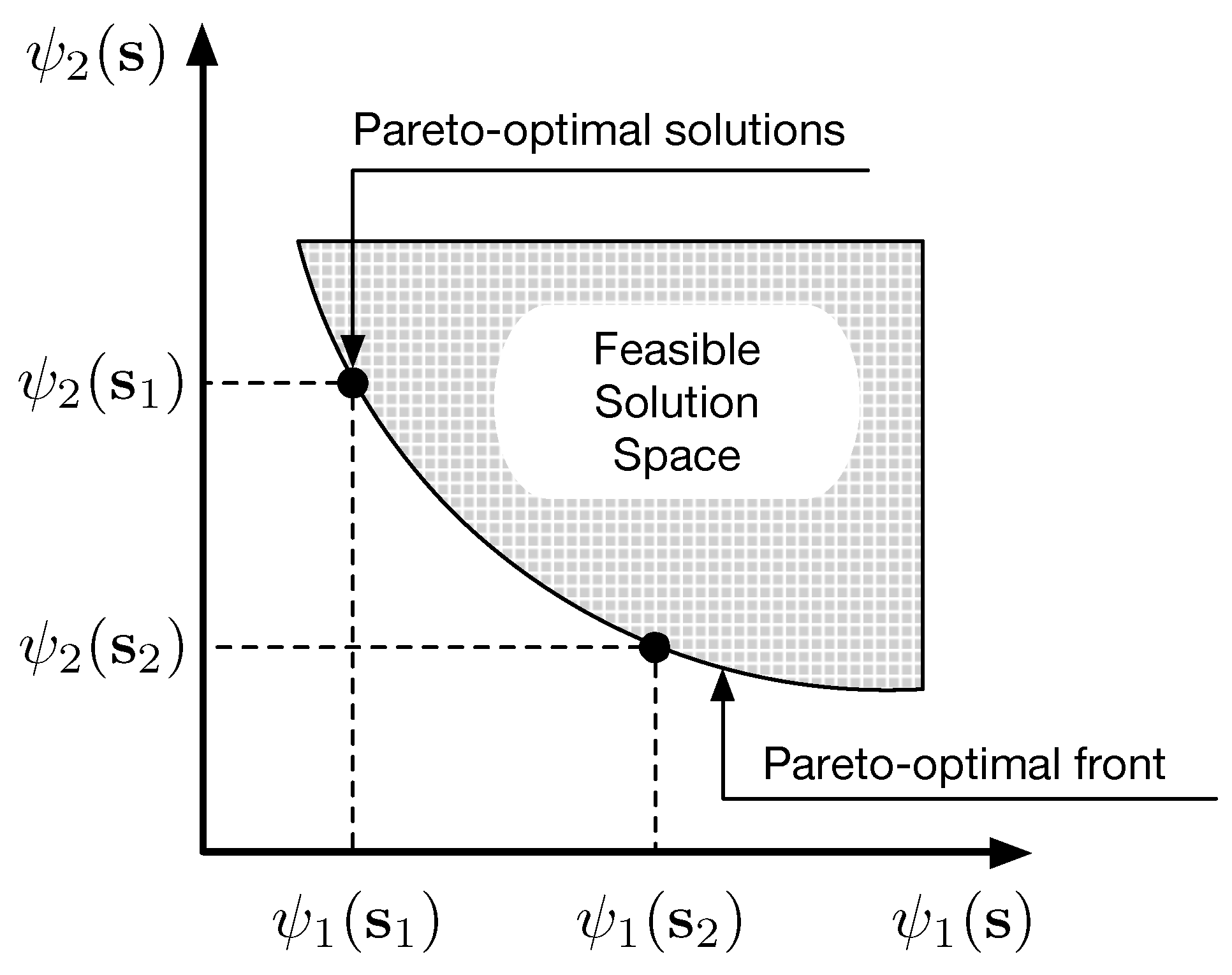
In this work, we use the Multi-Objective Genetic Algorithm (MOGA) [53], based on Genetic Algorithms (GAs) [54], to optimize, simultaneously, objective functions, that is, the global flow accuracy and the global byte accuracy, which will be further detailed in Section 4. The multi-objective optimization is performed by searching for the best set of parameters for the ELM and feature selection phases. The MOGA performs computer-based tasks that are based on the natural selection principle (e.g., mutation, selection, and crossover, among other procedures). The MOGA output is a set of pareto-optimal solutions, as can be seen in Figure 1. These are obtained from a set of feasible solutions, as illustrated in Figure 3 by the shaded area. The best optimal solutions (pareto-optimal solutions) are presented in the pareto-optimal front, or just the pareto front.
A trade-off is considered when maximizing multiple objective functions. In Figure 3, and are pareto-optimal solutions, and and are two objective functions. It is the task of an expert to decide between and , that is, considering a minimization problem, if is selected, then better rates of are obtained, when compared to . If another pareto-optimal solution is found, between and , and the user selects it, then one decides to have a more balanced solution. This way, the proposed method is capable of allowing users to adjust the classifier, in a flexible manner, by prioritizing byte, flow, or a balanced accuracy option between them. The choice could depend on the policies adopted by network administrators.
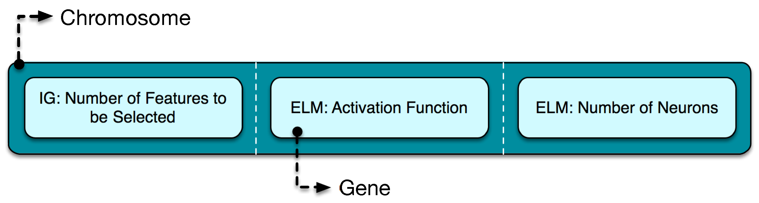
To simultaneously enhance both byte and flow accuracies, it is necessary to find the best set of parameters required for the machine learning algorithms. To achieve this, we chose to optimize both feature selection and conquering phases only. The dividing phase was not optimized to shorten the MOGA dimensional feature space (i.e., the search space). The chromosome used for the multi-optimization process can be visualized in Figure 4, composed of three genes, such as the two ELM parameters (i.e., the activation function and the hidden layer size (number of neurons)), and the number of features to be selected from a set of ranked features previously calculated by the Information Gain algorithm. The Information Gain algorithm (see Figure 1) is performed once, and a list of features with their respective values is presented. Multiple training executions (MOGA’s individuals and generations) are then performed to train the divide and conquer models, searching for the best pareto-optimal solutions and tested against a validation dataset, as will be further detailed in Section 4.1.3. For each execution, a different set of features previously calculated is selected (e.g., if number 10 is selected by the MOGA, for the feature selection gene, then the 10 highest valued features (based on the Information Gain score) are selected for the divide and conquer training processes). More details about the chromosome, including the MOGA parameters, and the lower and the upper bounds definition for each gene, can be seen in Section 4.
The chromosome, presented in Figure 4, has as input integer values only. This way, the mutation and crossover procedures from [55] were used, in order to deal with this mixed-integer multi-objective problem. The operators that must be changed are crossover and mutation ones [55]:
- Discrete crossover operator: If a discrete variable takes its values in a set , given two parents and such as and , a random number u is taken in and the indicesare generated, r being the rounding-off operator. This way, two children and with discrete variable and are produced, both and being in the range .
- Discrete mutation operator: A discrete variable is mutated replacing it by a randomly chosen element of set.
As already mentioned, the lower and the upper bounds definition for each gene will be discussed in Section 4. In a multi-objective approach, there is not a single optimal solution, but multiple optimal non-dominated solutions or pareto-optimal solutions, due to the trade-off that is considered when selecting the chromosomes within the pareto-optimal front (see Figure 3). This decision is up to the network administrator, as will be detailed in Section 4.2.2.
The MOGA algorithm was chosen for the multi-objective optimization process due to some of its benefits: (1) it is able to find, with a high probability, the best solution for an optimization problem, (2) it is a straightforward algorithm and relatively easy to implement, (3) it attempts to search the whole pareto front instead of one single pareto-optimal solution in each run, (4) it does not require any domain knowledge about the problem to be solved, and (5) it is not necessary to make any assumption about the pareto curve [56]. Nevertheless, the main drawback of MOGA is the lack of stability, due to its stochastic mechanism. This, however, could be tackled, for example, with game-theoretic approaches [57,58], including a hybrid approach with evolutionary algorithms [56]. In order to enhance our optimization process (e.g., stability [56] and techniques aiming at big data [59]), in the future we would like to perform experiments with other multi-objective optimization approaches [60,61,62,63].
3.5. Classification
The previous sections have detailed the proposed method, including a brief explanation of the machine learning algorithms used in this work. After training the algorithms, by following the experimental procedures detailed in Section 4, the MODC model is finally created. Actually, this model is composed of various models, that is, the GHSOM model and an ELM model for each GHSOM cluster, as seen in Figure 1. Once that training process is finished, the MODC model is prepared for the test phase, where novel and unknown instances are presented to the model to be classified as an application (e.g., Skype, BitTorrent, and Edonkey) or application protocol (e.g., HTTP, DNS, and FTP).
When in testing phase, the classifier captures the flows (e.g., pcap file) and transforms them into features during the pre-processing phase (see Section 4.1.2). A set of features is then generated, as detailed in Appendix A. During the training phase, a subset of features was chosen depending on the selected pareto-optimal solution. This subset is then passed as input to the GHSOM, which assigns clusters for each flow. Finally, the same subset of features is used as an input for an ELM model trained for the assigned cluster, which outputs an application or application protocol. Some of these flows are elephant flows, and the probability of correctly classifying these kind of flows is up to the network administrator, that must select a pareto-optimal solution (a simplified scenario is exemplified in Section 4.2.2). In Section 4, the test dataset labels are stored to evaluate the model’s classification performance. If the results are accurate, then the model is prepared to perform future classifications.
4. Experiments
This section describes the experimental settings, necessary for reproducibility, along with the experimental results, analysis, and comparisons.
4.1. Experimental Settings
The experimental settings section includes the dataset description, the pre-processing phase, the cross-validation methodology, the training parameters for reproducibility purpose, and the performance measures to evaluate the experiments.
4.1.1. Dataset
Public and private network traffic traces (datasets) have been used in the network traffic classification area of research. Private datasets hinder the reproducibility, making it infeasible for researchers to reproduce the results or even compare them against other methodologies. Additionally, most public datasets are not correctly labeled, i.e., without using a Ground-Truth (GT) process. The work in [64] pretends to be a first step towards the impartial validation of some DPI-based network traffic classifiers. The dataset is publicly available, the instances are correctly labeled by a reliable GT process, and the metrics and categorizations are well defined. In this work, the dataset is named CATALUNYA2013 [65], since it was assembled by researchers at the Universitat Politécnica de Catalunya. It was captured between 25 February 2013 and 1 May 2013 (66 days).
The authors in [64] generated the dataset by collecting flows from three operating systems (OS), based on the w3schools statistics (https://www.w3schools.com/browsers/browsers_os.asp) (most used OSs in January 2013): Windows XP, Windows 7, and Linux. Apple and mobile devices were not treated by the authors. The dataset was accurately labeled by the Volunteer-Based System (VBS), developed at Aalborg University [66]. It is a reliable labeling process since the flow is identified mainly by the operation system’s application process that generated the flow.
The dataset has 1,262,022 flows, but the authors were able to establish the GT for 535,438 flows only, since 520,993 flows were labeled by the application name tag and 14,445 flows could be identified based on the HTTP content-type header field. The remaining flows could not be identified since they presented a lifetime of less than 1 s, making VBS incapable of reliably labeling the application process [64]. Thus, only the reliable flows were used to train the MODC model and compare it against the DPI-based tools. The remaining flows were discarded. More details on the dataset can be found in [64,67].
The dataset flow distribution is described in Table 1. The flows are divided into 10 applications (e.g., Edonkey and BitTorrent) and application protocol (e.g., HTTP, FTP, and SSH) classes, along with an unknown class, which is labeled as unclassified. The RTMP traffic corresponds to Flash content that was generated by a web browser or a plugin.
4.1.2. Pre-Processing
The pre-processing is an important task in machine learning, aiming to prepare the data before training. The CATALUNYA2013 dataset was pre-processed, firstly transformed into flows by using the start and end timestamps defined in a log file, as described in [65]. This transformation and statistics generated from these flows were performed by the tools argus3 (http://qosient.com/argus/), yaf (https://tools.netsa.cert.org/yaf/docs.html) and ra (http://qosient.com/argus/ra.core.examples.shtml). Tools such as tstat (http://tstat.polito.it/index.shtml) could not be used, since some flows defined in the log file did not start with a formal TCP handshake. A total of 43 statistics attributes were extracted from the flows. The reader can refer to Appendix A for some brief descriptions. Attributes such as source and destination ports and IP addresses were discarded, since applications can encapsulate traffic into traditional protocols or make use of proxies. More information regarding such features can be obtained from the ra manual (http://qosient.com/argus/man/man1/ra.1.pdf).
The dataset values were then scaled within the range [0,1], with the objective of improving the performance and effectiveness of machine learning algorithms. The scaling process was performed with Equation (4), where is the scaled vector and is the data vector to be scaled. Furthermore, due to the imbalanced characteristic of the dataset, the process of random oversampling [68] was performed. The undersampling process could also be used, but it was avoided so that no important information would be lost. It is important to notice that this procedure was performed after the dividing process, for each individual partition, as will be presented in Section 4.1.3.
4.1.3. K-Fold Cross-Validation
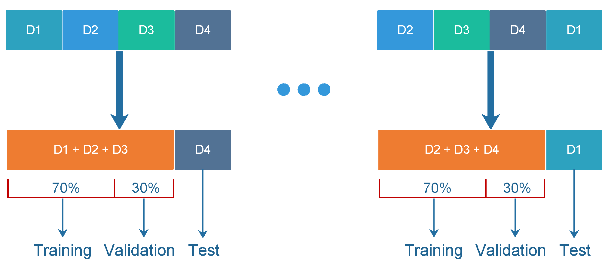
To evaluate the method, a k-fold cross-validation approach was performed with four folds (fourfold cross-validation), where each fold is an out-of-sample dataset at a time for testing purpose. In this paper, we named the folds as D1, D2, D3, and D4. The division of the four folds was performed randomly and in a stratified manner. During the testing phase, the final results are obtained by summing all confusion matrices from each testing fold and calculating the performance measures (Section 4.1.5) from this summed confusion matrix. This way, the complete dataset could be validated. This procedure was necessary since the DPI-based tools in [64] were tested against the full dataset (no prior training was necessary for these tools).
During the training process, by using the fourfold cross-validation procedure, for each training dataset (i.e., three folds), 70% of the dataset, stratified, was selected randomly for training, and 30% was for validation, as can be seen in Figure 5. This way, the MOGA could optimize the parameters by testing such a validation dataset. The training, validation, and testing phases were repeated four times, as seen in Figure 5. Each partition was tested separately. Finally, as already mentioned, the complete dataset was fully tested, and the results could be compared with DPI-based tools, as well as with some machine learning-based methods.
4.1.4. Training Parameters
When the dataset is correctly treated for the training, validation, testing, and optimization phases, the next step is to prepare for the training process. The machine learning algorithms used in our methodology require setting some training parameters. It is important to notice that the training and optimization processes should occur four times, by following the k-fold cross-validation method presented in Section 4.1.3.
Since the Information Gain algorithm ranks the features by relevance order, that is, by quality order, it is yet necessary to choose a subset from the highest ranked features and, for that reason, the MOGA was applied to the feature selection process to choose the subset from a total of 43 features (see Section 4.1.2). The MOGA will determine the best subset from a set of pareto-optimal solutions obtained during the training, by testing each solution against the validation dataset presented in Section 4.1.3.
The optimization, along with all the experimental phases, were conducted by MATLAB working in a distributed manner. A total of 9 CPU cores were used, distributed among three machines, each with 30GB of RAM memory and with a single core responsible for testing one GA individual within a population. Our fitness function, with chromosome previously presented in Figure 4, has as input integer values only. This way, the mutation and crossover procedures from [55] were used. During the experiments, it was observed that, after the 20th generation, no considerable changes in results were detected. Therefore, a stall generation limit was set to 30 and a maximum generation set to 50. The pareto fraction was set to 0.35 (MATLAB defaults); that is, only 35% of the individuals from the pareto front of the current population are selected. The population size was set to 18 due to RAM memory limitation, since each chromosome utilized almost 10 GB of RAM because of the dataset number of instances and dimension size. Thus, each core occupied almost 10 GB of the machine’s memory resource. As already discussed, in a nutshell, the chromosome was composed of the ELM activation function, the ELM number of neurons, and the number of features to be selected from a set of ranked features, previously pre-selected by the Information Gain algorithm.
With regard to the GHSOM algorithm, all parameters were set to their default values according to the GHSOM Matlab ToolBox (http://www.ofai.at/~elias.pampalk/ghsom/download.html), that is, Gaussian for the neighborhood function, (depth) and (breadth). For the ELM, we aim to optimize the activation function and the number of neurons. The functions Sigmoidal, Sine, Hardlim, Triangular Basis, and Radial Basis were considered. For the number of neurons, a range of [10, 400] was set as lower and upper boundaries.
4.1.5. Performance Measures
This work was evaluated using the performance measures described in Table 2. The flow and byte accuracies were named Global Flow Accuracy and Global Byte Accuracy, respectively, since they should be calculated globally, regardless of the class. These are the measures to be optimized in this work. The per-class flow and byte accuracies were treated by the Recall measure, with each class being represented by , where M is the total number of classes. The measures the classifier’s fidelity for each class i. is the total number of correctly classified flows, globally, and represents the flows that were correctly classified for each class i. Finally, n is the total number of flows, globally, and is the total number of flows presented in class i.
The work in [64] considers the , , and in their experiments only. This paper introduces more performance measures in order to fully investigate the MODC model quality.
4.2. Experimental Results
In this section, the experimental results will be presented and analyzed, including some comparisons to validate the model.
4.2.1. Analysis of the Divide and Conquer Strategy
Before presenting the MODC results, we should investigate the results for the divide and conquer strategy only, without the optimization process, to verify whether this can actually enhance the quality of a classification model. We compare two different models. The first is a single expert model (SEM), where an ELM model is trained. The second is a divide and conquer model (DCM), as seen in Section 3, but without the optimization process.
Both models were trained with the dataset presented in Section 4.1.1, but without the k-fold cross-validation, to simplify the comparison. The dataset was then randomized and divided: 70% for training and 30% for testing (stratified). A total of 16 training and testing procedures was performed for both methods, by varying the number of ELM neurons and the number of features to be selected by the Information Gain, assuming the values {200, 400, 600, and 800} and {10, 20, 30, and 40}, respectively.
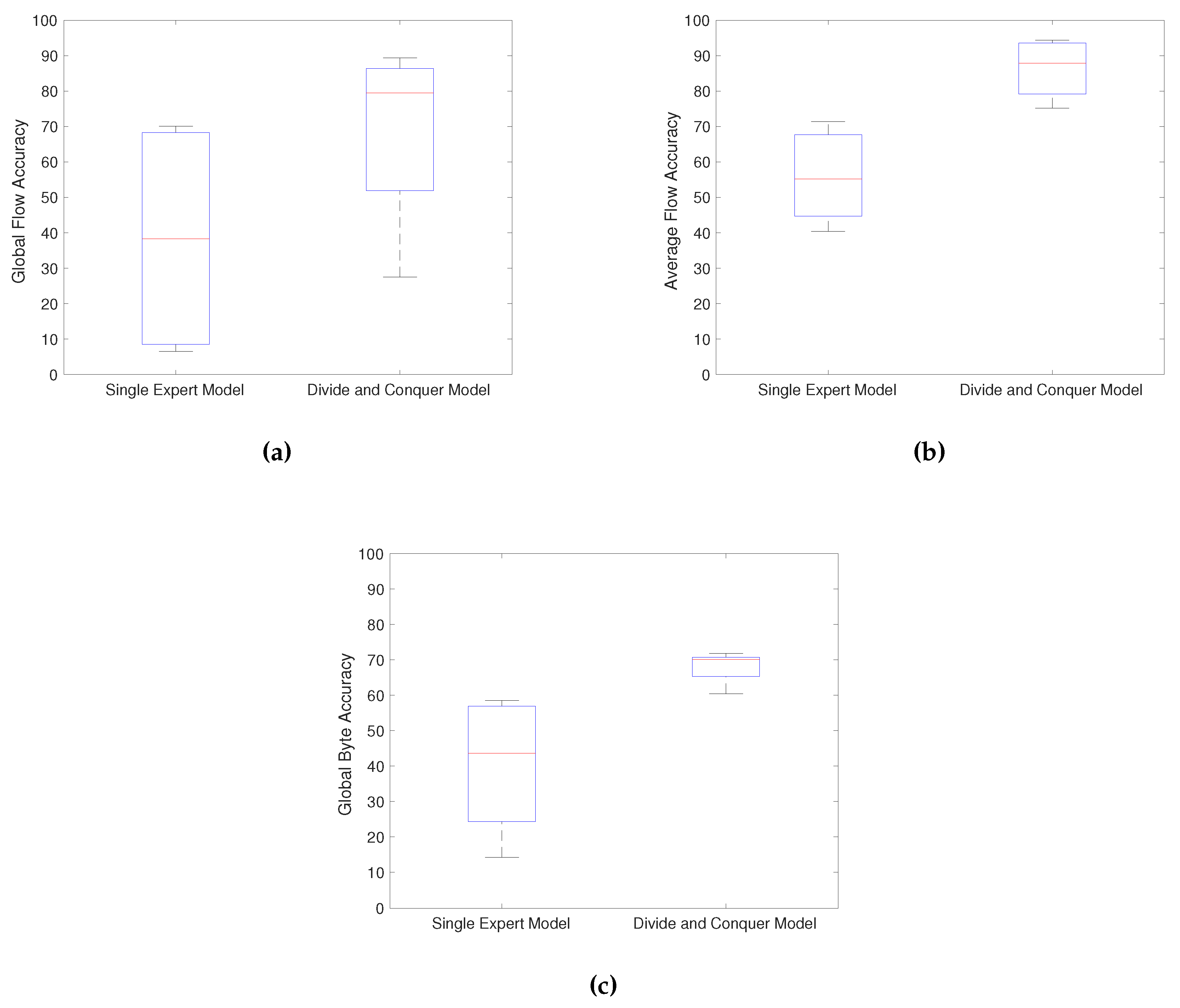
The results for , , and can be seen in Figure 6a, Figure 6b, and Figure 6c, respectively. Observe that the median values are superior in the divide and conquer model. Besides that, for and , the DCM’s minimal values were superior to the SEM’s maximal values. Based on the boxplots results, we conclude that the divide and conquer strategy is superior to a single expert model. The results can be further enhanced by optimizing these assumed parameters, focusing on the and measures, with the aid of the MOGA. This also enables network administrators to select the best settings according to their needs, by prioritizing flow or byte accuracies.
4.2.2. Analysis of the Pareto-Optimal Solutions
After the training and optimization processes, the best set of parameters are found, and four dataset partitions should be tested, according to the k-fold cross-validation process presented in Section 4.1.3. This can also be visualized in Figure 5. In other words, the datasets D1, D2, D3, and D4 were tested with the best set of parameters, that is, the best pareto-optimal solutions obtained by the MOGA optimization during four training processes.
It is important to emphasize that the pareto-optimal solutions obtained by the training and optimization of the model with the dataset D1 + D2 + D3 should be different from what is obtained by doing the same process for the dataset D2 + D3 + D4. Therefore, by following this procedure, the testing results for datasets D1, D2, D3, and D4 can be visualized in Table 3 and Table 4, for the best pareto-optimal solution for the measures and , respectively. Additionally, the best parameters found by the MOGA for the ELM number of neurons (# Neurons), ELM activation function (Act. Func.), and the number of features to be used from the Information Gain ranking (# Features) are shown. The intermediate pareto-optimal solutions were discarded, since we aim to analyze the best solutions for each metric only, but it could be available for the network administrators to select a more balanced solution between flow and byte accuracies.
In Table 3, the column D1 shows the parameters obtained from the pareto-optimal solution with the highest found during optimization of the training dataset (i.e., D2 + D3 + D4) and the performance results when the generated model was tested against the D1 (out-of-sample) dataset. The same process occurs with the remaining columns, with each column dataset being the out-of-sample at a given time. Note that a high number of features was selected, indicating that almost all features were necessary to reach higher values of . It can also be observed that the presented results below 80%.
The best pareto-optimal solutions were also selected. The results can be visualized in Table 4. It can be observed that, when compared to Table 3, the number of features has decreased, together with the and , and the performance has improved due to the selected solutions, prioritizing the byte accuracy. The results differ depending on the pareto-optimal solution to be selected, which should be the task of network administrators, according to their needs, turning this into a flexible (adjustable) hybrid model.
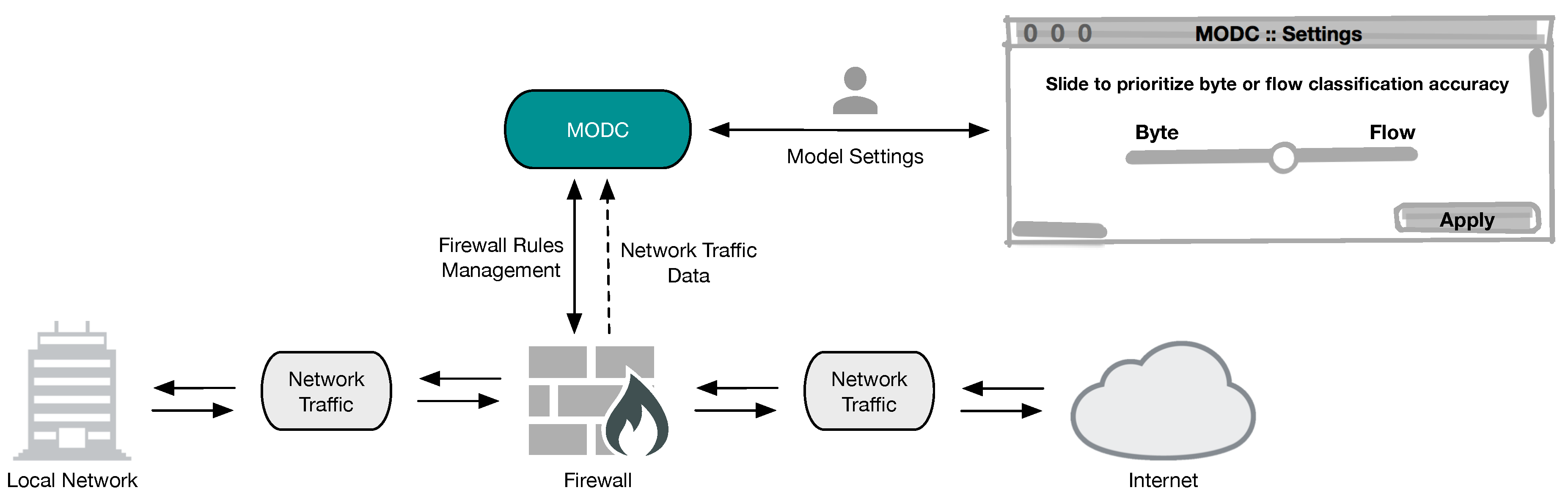
Based on the statistics presented by the MODC, generated from a given network traffic data, firewall rules can be created (manually or automatically) to block unwanted network traffic, as exemplified in Figure 7. The pareto-optimal selection process can be simplified for the network administrator with the use, for example, of a settings window, with the pareto-optimal solutions being selected through a slider controller, as seen in Figure 7, depending on the network necessity. After the selection and confirmation, the stored model, previously trained with the optimal parameters, is then selected to classify real time network traffic. This decision can impact the Quality of Service (QoS) of a network, by sending a firewall instruction to prioritize the blocking of unwanted elephant flows (e.g., on low bandwidth networks), unwanted general flows (e.g., network policy violations data) or a more balanced decision.
4.2.3. Execution Time
The execution time (in seconds) for the training, optimization, and classification phases can be visualized in Table 5. The GHSOM and ELM training were performed several times, and the results for the mean and standard error of the mean (95% confidence interval) are presented. Note that the GHSOM is about 7–9 times slower than the ELM training runtime. This impacted the MOGA optimization runtime, which, according to the results, took almost one and a half days to execute for each of the four partitions. Nevertheless, the classification runtime reached fast performance, with a mean of 133.859 instances (for each partition) being classified in less than 17 s; that is, the trained model (classifier) classified about 8.070 flows per second. This can be enhanced by using a lighter and compiled version of the model (e.g., C++), instead of using interpreted MATLAB library calls.
4.2.4. Comparison between the MODC Model and DPI-Based Tools
The proposed method (MODC) was also compared to six popular DPI-based tools, including two commercial ones (PACE (https://www.ipoque.com/products/dpi-engine-rsrpace-2) and NBAR (http://www.cisco.com/c/en/us/products/ios-nx-os-software/network-based-application-recognition-nbar/index.html) and four free tools (OpenDPI (http://code.google.com/p/opendpi/), l7-filter (http://l7-filter.sourceforge.net), NDPI (http://www.ntop.org/products/deep-packet-inspection/ndpi/), and Libprotoident (https://research.wand.net.nz/software/libprotoident.php)). The results from these tools were obtained from [64], where the “App.” corresponds to the application or application protocol and “Clas.” column corresponds to the classifier. The authors conducted the analysis by investigating three metrics only, the Recall in Flows (), and , in order to evaluate the DPI-based tools’ performance. The comparison of our method to these tools can be visualized in Table 6. The Correct (Cor.) column in [64] corresponds to the Recall in this paper. The remaining columns are the Wrong (Wro.), when the flow is incorrectly classified as another application and Unclassified (Unc.), when the flow is classified as unknown. It is important to notice that we aim to compare the results for flow accuracy only, since the authors in [64] did not analyze the byte accuracy.
From Table 6, it can be observed that, for 8 out of 10 applications, the proposed method (MODC) results exceeded 92% of accuracy, presenting good performance when compared to other DPI-based tools. The FTP and RTMP results were average due to their small number of flows in the dataset (see Table 1). This implicates directly in the model training, decreasing the classification performance.
In order to select the best classifier, the authors in [64] utilize the as the determinant measure. Note that, in Table 7, the MODC presented the best value for , outperforming all DPI-based tools. On the other hand, our proposed method was the third best classifier when evaluating the , but with results not far from the best classifier, the PACE (commercial). Nevertheless, as mentioned before, the MODC model has other advantages when compared to DPI-based tools, such as the capability of classifying encrypted data, better classification speed performance, and no violation of users’ data privacy, since no payload is required. Additionally, in Table 7, observe that other tools obtained poor performance results for and .
4.2.5. A Deeper Analysis
The previous sections have shown that the divide and conquer strategy can enhance the model quality, by dividing a complex problem into simpler problems and creating experts for each subproblem. A multi-objective optimization was thus performed to optimize both flow and byte accuracies. The comparisons, regarding average flow accuracy, have shown that our proposed method is superior to the DPI-based tools analyzed, including the commercial ones, for the dataset being tested.
As already discussed, the authors in [64] conducted the experiments with three performance measures only: Recall in Flows (), , and . These measures are important in order to analyze a classifier’s quality, but they are incomplete when analyzed alone. In this section, we also investigate the MODC performance when analyzed with four other measures: Precision, Average Precision Accuracy (), Global Byte Accuracy (), and Recall in Bytes (). The precision is an important metric to be analyzed along with the recall, for each particular class. Good rates of recall do not necessarily indicate that the classifier is precise, due to the likely presence of false positives.
Additionally, in this section, inspired by the divide and conquer strategy, we consider dividing the dataset into two parts, splitting it by transport layer protocol. The dataset was divided into UDP and TCP datasets, to verify whether the results could be improved. This way, a variant of the MODC is proposed, the Multiple MODC (M-MODC), where an MODC model is created for each dataset partition, that is, an MODC for the UDP dataset and another one for the TCP dataset. To simplify the analysis and comparisons, the MODC model, applied to the full dataset (without the transport layer protocol splitting), will be named S-MODC (Single MODC). Another reason for the dividing was that some features were generated exclusively for TCP, making the UDP instances filled up with null feature values and interfering during the learning process.
The results for the S-MODC can be visualized in Table 8. Note that the RF values are the same as those of the Correct column in Table 6. Although the results for the show accurate results, few can be observed in precision and . Nevertheless, note that poor results of precision were observed in classes with few instances in the dataset and that poor results of were observed on Edonkey and BitTorrent classes, that is, mainly UDP traffic. The precision rates could be enhanced by adding more instances to those with few examples. The transport layer issue was tackled by creating two distinct S-MODC models, the M-MODC, that is, by creating an S-MODC model for UDP and another for TCP traffic.
The results for the M-MODC can be visualized in Table 9. Observe that, in this case, the results for precision continue to present some poor values due to the lack of instances, but show an increase in performance regarding the . In order to compare both methods, a summary of the results can be visualized in Table 10. The results for both methods did not present considerable differences, with exception to the , which showed to be far superior in the M-MODC method. It is important to notice that, regarding this comparison, the best flow pareto-optimal solution was selected for analysis. When compared to the DPI-based tools, the M-MODC is the second best classifier ( measure), behind the commercial PACE only. Nevertheless, as already discussed, our method brings many advantages when compared to the DPI-based method.
4.2.6. Comparison with Other Machine Learning Methods
We also benchmarked the S-MODC and M-MODC against some machine learning methods, such as the ELM, this time performed using the k-fold cross validation, Naïve Bayes, k-Nearest Neighbors (kNN), C4.5, and Softmax Layer. All the experiments were conducted using the k-fold cross validation as described in Section 4.1.3. This way, the same test dataset was utilized for all the methods.
The same pre-processed dataset, as described in this paper, was used to train the models. The algorithms were obtained from the official MATLAB toolboxes, with the exception of ELM (http://www.ntu.edu.sg/home/egbhuang/elm_codes.html). It was not the purpose of this paper to exhaustively train such models with multiple parameters, or even to propose hybrid methods with most of them (e.g., by using optimizers), then, for that reason, the default parameters for each algorithm, defined at the official toolboxes’ web pages for the Naïve Bayes (https://www.mathworks.com/help/stats/fitcnb.html), kNN (https://www.mathworks.com/help/stats/fitcknn.html), C4.5 (https://www.mathworks.com/help/stats/fitctree.html), and Softmax Layer (https://www.mathworks.com/help/nnet/ref/trainsoftmaxlayer.html), were used in the experiments. For the ELM, we used 400 neurons to train the model and the sigmoidal function.
The benchmark results are shown in Table 11. Observe that both of our methods outperformed all the analyzed methods, with the exception of the , that presented slightly better results with the C4.5 algorithm. Nonetheless, the other methods obtained poor performance of , due to the fact that our methods are able to optimize, simultaneously, both the and the performance measures.
5. Conclusions
This work proposed a Multi-Objective Divide and Conquer (MODC) model by combining supervised and unsupervised machine learning techniques, such as the Growing Hierarchical Self-Organizing Maps (GHSOM), the Extreme Learning Machine (ELM), the Multi-objective Genetic Algorithm (MOGA), and the Information Gain for feature selection, into a flexible hybrid model, to deal with the problem of network traffic classification. It is based on the divide and conquer strategy proposed by [36]. This approach proved to enhance the learning process.
The dividing process is led by an unsupervised algorithm, the Growing Hierarchical Self-Organizing Map (GHSOM), and focuses on the division of a large and complex problem into smaller and simpler problems (tasks), being represented by clusters. The conquer process then attacks the less complex tasks (smaller datasets or clusters) by a supervised learning algorithm, the Extreme Learning Machine (ELM). Some processes are then optimized by the MOGA algorithm. To the best of our knowledge, there are no contributions that investigate the use of a divide and conquer strategy for network traffic classification, along with the flexibility of allowing network administrators to choose the best parameters for their networks, by prioritizing flow or byte classification accuracy. This can be performed with the use of multi-objective optimization, by selecting between pareto-optimal solutions. Additionally, this work is compared against commonly used network traffic classifiers (DPI-based tools) and some machine learning algorithms, whose results could benefit the benchmarking against different methodologies.
The MODC presented promising results in the experiments, with an average flow accuracy of 94.14%, exceeding the performance of all DPI-based tools analyzed, including the commercial tools, and outperforming five machine learning-based methods. Additionally, a variant of the MODC was proposed, the Multiple MODC (M-MODC), to deal with the lack of feature values in the UDP transport layer protocol. The M-MODC performance showed to be superior to the Single MODC (S-MODC) concerning the global byte accuracy, presenting results of, approximately, 90%. Although promising results were obtained in both byte and flow accuracies, the average precision accuracy reached an average performance of 70.11% for the M-MODC method due to the lack of instances for particular classes in the analyzed dataset, that is, due to the imbalanced dataset. Nevertheless, this can be enhanced by collecting more instances of those classes with few examples.
For future research, online machine learning techniques could be used to improve the results and should be investigated, since network traffic’s behavior frequently changes over time. These techniques allow one to train a model as soon as new instances are presented to the system, incrementally. Additionally, semi-supervised algorithms could be utilized, since they allow us the use of a few labeled instances plus many unlabeled instances (easily collected), which benefits the training of imbalanced datasets. Studies can also be performed on networks with high throughput (e.g., networks with throughput of 10 Gbps or higher) with the aid of big data techniques, cloud computing with multiple computing nodes, and deep learning.
Author Contributions
Z.N. conceived and wrote this paper; D.S. reviewed this paper and provided ideas and suggestions.
Acknowledgments
The authors would like to thank the Broadband Communications Research Group at Universitat Politècnica de Catalunya for providing the dataset.
Conflicts of Interest
The authors declare no conflict of interest.
Appendix A. Extracted Features
| Feature | Description |
| Proto | Transaction protocol |
| sTtl | Src dst TTL value |
| dTtl | Dst src TTL value |
| TotPkts | Total transaction packet count |
| SrcPkts | Src dst packet count |
| DstPkts | Dst src packet count |
| TotBytes | Total transaction bytes |
| SrcBytes | Src dst transaction bytes |
| DstBytes | Dst src transaction bytes |
| TotAppBytes | Total application bytes |
| SAppBytes | Src dst application bytes |
| DAppBytes | Dst src application bytes |
| Load | Bits per second |
| SrcLoad | Source bits per second |
| DstLoad | Destination bits per second |
| Loss | Pkts retransmitted or dropped |
| SrcLoss | Source pkts retransmitted or dropped |
| DstLoss | Destination pkts retransmitted or dropped |
| pLoss | Percent pkts retransmitted or dropped |
| SrcGap | Source bytes missing in the data stream |
| DstGap | Destination bytes missing in the data stream |
| Rate | Pkts per second |
| SrcRate | Source pkts per second |
| DstRate | Destination pkts per second |
| SIntPkt | Source interpacket arrival time (mSec) |
| SIntPktAct | Source active interpacket arrival time (mSec) |
| SIntPktIdl | Source idle interpacket arrival time (mSec) |
| DIntPkt | Destination interpacket arrival time (mSec) |
| DIntPktAct | Destination active interpacket arrival time (mSec) |
| DIntPktIdl | Destination idle interpacket arrival time (mSec) |
| TcpRtt | TCP connection setup round-trip time, the sum of “synack” and “ackdat” |
| SynAck | TCP conn. setup time, the time between the SYN and the SYN_ACK packets |
| AckDat | TCP conn. setup time, the time between the SYN_ACK and the ACK packets |
| sMaxPktSz | Maximum packet size for traffic transmitted by the src |
| dMaxPktSz | Maximum packet size for traffic transmitted by the dst |
| sMinPktSz | Minimum packet size for traffic transmitted by the src |
| dMinPktSz | Minimum packet size for traffic transmitted by the dst |
| Dur | Record total duration |
| RunTime | Total active flow run time |
| Mean | Average duration of aggregated records |
| Sum | Total accumulated durations of aggregated records |
| Min | Minimum duration of aggregated records |
| Max | Maximum duration of aggregated records |
References
- Wang, Y.; Ke, W.; Tao, X. A feature selection method for large-scale network traffic classification based on Spark. Information 2016, 7, 6. [Google Scholar] [CrossRef]
- Ertam, F.; Avcı, E. A new approach for internet traffic classification: GA-WK-ELM. Measurement 2017, 95, 135–142. [Google Scholar] [CrossRef]
- Schmidt, B.; Al-Fuqaha, A.; Gupta, A.; Kountanis, D. Optimizing an artificial immune system algorithm in support of flow-Based internet traffic classification. Appl. Soft Comput. 2017, 54, 1–22. [Google Scholar] [CrossRef]
- Shi, H.; Li, H.; Zhang, D.; Cheng, C.; Wu, W. Efficient and robust feature extraction and selection for traffic classification. Comput. Netw. 2017, 119, 1–16. [Google Scholar] [CrossRef]
- Peng, L.; Zhang, H.; Chen, Y.; Yang, B. Imbalanced traffic identification using an imbalanced data gravitation-based classification model. Compet. Comm. 2017, 102, 177–189. [Google Scholar] [CrossRef]
- Gómez, S.E.; Martínez, B.C.; Sánchez-Esguevillas, A.J.; Hernández Callejo, L. Ensemble network traffic classification: Algorithm comparison and novel ensemble scheme proposal. Comput. Netw. 2017, 127, 68–80. [Google Scholar] [CrossRef]
- Ijaz, S.; Hashmi, F.A.; Asghar, S.; Alam, M. Vector Based Genetic Algorithm to optimize predictive analysis in network security. Appl. Intell. 2017, 48, 1086–1096. [Google Scholar] [CrossRef]
- Benmessahel, I.; Xie, K.; Chellal, M. A new evolutionary neural networks based on intrusion detection systems using multiverse optimization. Appl. Intell. 2017, 48, 2315–2327. [Google Scholar] [CrossRef]
- Hajjar, A.; Khalife, J.; Díaz-Verdejo, J. Network traffic application identification based on message size analysis. J. Netw. Comput. Appl. 2015, 58, 130–143. [Google Scholar] [CrossRef]
- Peng, L.; Yang, B.; Chen, Y. Effective packet number for early stage internet traffic identification. Neurocomputing 2015, 156, 252–267. [Google Scholar] [CrossRef]
- Divakaran, D.M.; Su, L.; Liau, Y.S.; Vrizlynn, V.L. SLIC: Self-Learning Intelligent Classifier for network traffic. Comput. Netw. 2015, 91, 283–297. [Google Scholar] [CrossRef]
- Alshammari, R.; Nur Zincir-Heywood, A. Identification of VoIP encrypted traffic using a machine learning approach. J. King Saud Univ. Comput. Inf. Sci. 2015, 27, 77–92. [Google Scholar] [CrossRef]
- Megyesi, P.; Szabó, G.; Molnár, S. User behavior based traffic emulator: A framework for generating test data for DPI tools. Comput. Netw. 2015, 92, 41–54. [Google Scholar] [CrossRef]
- Bujlow, T.; Carela-Español, V.; Barlet-Ros, P. Independent comparison of popular DPI tools for traffic classification. Comput. Netw. 2015, 76, 75–89. [Google Scholar] [CrossRef] [Green Version]
- Singh, R.; Kumar, H.; Singla, R.K. An intrusion detection system using network traffic profiling and online sequential extreme learning machine. Expert Syst. Appl. 2015, 42, 8609–8624. [Google Scholar] [CrossRef]
- Rizzi, A.; Iacovazzi, A.; Baiocchi, A.; Colabrese, S. A low complexity real-time Internet traffic flows neuro-fuzzy classifier. Comput. Netw. 2015, 91, 752–771. [Google Scholar] [CrossRef]
- Namdev, N.; Agrawal, S.; Silkari, S. Recent Advancement in Machine Learning Based Internet Traffic Classification. Procedia Comput. Sci. 2015, 60, 784–791. [Google Scholar] [CrossRef]
- Biswas, A.R.; Giaffreda, R. IoT and Cloud Convergence: Opportunities and Challenges. In Proceedings of the 2014 IEEE World Forum on Internet of Things (WF-IoT), Seoul, Korea, 6–8 March 2014. [Google Scholar]
- Tsiropoulou, E.E.; Paruchuri, S.T.; Baras, J.S. Interest, energy and physical-aware coalition formation and resource allocation in smart IoT applications. In Proceedings of the 2017 51st Annual Conference on Information Sciences and Systems (CISS), Baltimore, MD, USA, 22–24 March 2017. [Google Scholar]
- Meidan, Y.; Bohadana, M.; Shabtai, A.; Guarnizo, J.D.; Ochoa, M.; Ole Tippenhauer, N.; Elovici, Y. ProfilIoT: A Machine Learning Approach for IoT Device Identification Based on Network Traffic Analysis. In Proceedings of the Symposium on Applied Computing (ACM), Marrakech, Morocco, 3–7 April 2017. [Google Scholar]
- Diro, A.A.; Chilamkurti, N. Distributed attack detection scheme using deep learning approach for Internet of Things. Future Gener. Comput. Syst. 2018, 82, 761–768. [Google Scholar] [CrossRef]
- Kim, J.Y.; Bu, S.J.; Cho, S.B. Zero-day malware detection using transferred generative adversarial networks based on deep autoencoders. Informing Sci. 2018, 460–461, 83–102. [Google Scholar] [CrossRef]
- Kozik, R. Distributing extreme learning machines with Apache Spark for NetFlow-based malware activity detection. Pattern Recogn. Lett. 2018, 101, 14–20. [Google Scholar] [CrossRef]
- Zhang, Q.; Yang, L.T.; Chen, Z.; Li, P. A survey on deep learning for big data. Inf. Fusion 2018, 42, 146–157. [Google Scholar] [CrossRef]
- Boutaba, R.; Salahuddin, M.A.; Limam, N.; Ayoubi, S.; Shahriar, N.; Estrada-solano, F.; Caicedo, O.M. A comprehensive survey on machine learning for networking: Evolution, applications and research opportunities. J. Internet Serv. Appl. 2018, 9, 16. [Google Scholar] [CrossRef]
- Antonello, R.; Fernandes, S.; Kamienski, C.; Sadok, D.; Kelner, J.; Gódor, I.; Szabó, G.; Westholm, T. Deep packet inspection tools and techniques in commodity platforms: Challenges and trends. J. Netw. Comput. Appl. 2012, 35, 1863–1878. [Google Scholar] [CrossRef]
- La Mantia, G.; Rossi, D.; Finamore, A.; Mellia, M.; Meo, M. Stochastic Packet Inspection for TCP Traffic. In Proceedings of the 2010 IEEE International Conference on Communications, Cape Town, South Africa, 23–27 May 2010; pp. 1–6. [Google Scholar]
- Sun, G.; Dong, H.; Li, D.; Xiao, F. NTCA: A high-performance network traffic classification architecture. Int. J. Future Gener. Commun. Netw. 2013, 6, 11–20. [Google Scholar] [CrossRef]
- Fernandes, S.; Antonello, R.; Lacerda, T.; Santos, A.; Sadok, D.; Westholm, T. Slimming Down Deep Packet Inspection Systems. In Proceedings of the IEEE INFOCOM Workshops 2009, Rio de Janeiro, Brazil, 19–25 April 2009; pp. 1–6. [Google Scholar]
- Callado, A.; Kelner, J.; Sadok, D.; Alberto Kamienski, C.; Fernandes, S. Better network traffic identification through the independent combination of techniques. J. Netw. Comput. Appl. 2010, 33, 433–446. [Google Scholar] [CrossRef]
- Khalife, J.; Hajjar, A.; Díaz-Verdejo, J.E. A multilevel taxonomy and requirements for an optimal traffic-classification model. Int. J. Netw. Manag. 2014, 24, 101–120. [Google Scholar] [CrossRef]
- Nascimento, Z.; Sadok, D.; Fernandes, S. Comparative study of a Hybrid Model for network traffic identification and its optimization using Firefly Algorithm. In Proceedings of the 2013 IEEE Symposium on Computers and Communications (ISCC), Split, Croatia, 7–10 July 2013; pp. 000862–000867. [Google Scholar]
- Shi, H.; Li, H.; Zhang, D.; Cheng, C.; Cao, X. An efficient feature generation approach based on deep learning and feature selection techniques for traffic classification. Comput. Netw. 2018, 132, 81–98. [Google Scholar] [CrossRef]
- Liu, Z.; Wang, R.; Tao, M.; Cai, X. A class-oriented feature selection approach for multi-class imbalanced network traffic datasets based on local and global metrics fusion. Neurocomputing 2015, 168, 365–381. [Google Scholar] [CrossRef]
- Dainotti, A.; Pescape, A.; Claffy, K. Issues and future directions in traffic classification. IEEE Netw. 2012, 26, 35–40. [Google Scholar] [CrossRef] [Green Version]
- Jacobs, R.A.; Jordan, M.I.; Nowlan, S.J.; Hinton, G.E. Adaptive Mixtures of Local Experts. Neural. Comput. 1991, 3, 79–87. [Google Scholar] [CrossRef]
- Rauber, A.; Merkl, D.; Dittenbach, M. The growing hierarchical self-organizing map: Exploratory analysis of high-dimensional data. IEEE Trans. Neural Netw. 2002, 13, 1331–1341. [Google Scholar] [CrossRef] [PubMed]
- Huang, G.B.; Zhu, Q.Y.; Siew, C.K. Extreme learning machine: Theory and applications. Neurocomputing 2006, 70, 489–501. [Google Scholar] [CrossRef] [Green Version]
- Wang, R.Y.; Liu, Z.; Zhang, L. Method of data cleaning for network traffic classification. J. China Univ. Posts Telecommun. 2014, 21, 35–45. [Google Scholar] [CrossRef]
- Nascimento, Z.; Sadok, D.; Fernandes, S. A Hybrid Model for Network Traffic Identification Based on Association Rules and Self-Organizing Maps (SOM). In Proceedings of the Ninth International Conference on Networking and Services, ICNS 2013, Lisbon, Portugal, 24–29 March 2013; pp. 213–219. [Google Scholar]
- Nascimento, Z.; Sadok, D.; Fernandes, S.; Kelner, J. Multi-objective optimization of a hybrid model for network traffic classification by combining machine learning techniques. In Proceedings of the 2014 International Joint Conference on Neural Networks (IJCNN), Beijing, China, 6–11 July 2014; pp. 2116–2122. [Google Scholar]
- Zhang, J.; Xiang, Y.; Zhou, W.; Wang, Y. Unsupervised traffic classification using flow statistical properties and {IP} packet payload. J. Comput. Syst. Sci. 2013, 79, 573–585. [Google Scholar] [CrossRef]
- Huang, S.Y.; Huang, Y.N. Network traffic anomaly detection based on growing hierarchical SOM. In Proceedings of the 2013 43rd Annual IEEE/IFIP International Conference on Dependable Systems and Networks (DSN), Budapest, Hungary, 24–27 June 2013; pp. 1–2. [Google Scholar]
- Liu, Y.; Li, W.; Li, Y.C. Network Traffic Classification Using K-means Clustering. In Proceedings of the Second International Multi-Symposiums on Computer and Computational Sciences (IMSCCS 2007), Iowa City, IA, USA, 13–15 August 2007; pp. 360–365. [Google Scholar]
- Li, D.; Hu, G.; Wang, Y.; Pan, Z. Network traffic classification via non-convex multi-task feature learning. Neurocomputing 2015, 152, 322–332. [Google Scholar] [CrossRef]
- Lin, G.Z.; Xin, Y.; Niu, X.X.; Jiang, H.B. Network traffic classification based on semi-supervised clustering. J. China Univ. Posts Telecommun. 2010, 17, 84–88. [Google Scholar] [CrossRef]
- De La Hoz, E.; De La Hoz, E.; Ortiz, A.; Ortega, J.; Martínez-Álvarez, A. Feature selection by multi-objective optimisation: Application to network anomaly detection by hierarchical self-organising maps. Knowl. Based Syst. 2014, 71, 322–338. [Google Scholar] [CrossRef]
- Ostaszewski, M.; Bouvry, P.; Seredynski, F. Multiobjective classification with moGEP: An application in the network traffic domain. In Proceedings of the 11th Annual Conference on Genetic and Evolutionary Computation, Montreal, QC, Canada, 8–12 July 2009; pp. 635–642. [Google Scholar]
- Bacquet, C.; Zincir-Heywood, A.N.; Heywood, M.I. Genetic optimization and hierarchical clustering applied to encrypted traffic identification. In Proceedings of the 2011 IEEE Symposium on Computational Intelligence in Cyber Security (CICS), Paris, France, 11–15 April 2011; pp. 194–201. [Google Scholar]
- Mitchell, T.M. Machine Learning; McGraw-Hill, Inc.: New York, NY, USA, 1997. [Google Scholar]
- Fayyad, U.M.; Irani, K.B. Multi-Interval Discretization of Continuous-Valued Attributes for Classification Learning. In Proceedings of the 13th International Joint Conference on Uncertainly in Artificial Intelligence (IJCAI93), Chambery, France, 28 August–3 September 1993; pp. 1022–1029. [Google Scholar]
- Kohonen, T. The Self-Organizing Map. Proc. IEEE 1990, 78, 1464–1480. [Google Scholar] [CrossRef]
- Konak, A.; Coit, D.W.; Smith, A.E. Multi-objective optimization using genetic algorithms: A tutorial. Reliab. Eng. Syst. Saf. 2006, 91, 992–1007. [Google Scholar] [CrossRef]
- Holland, J.H. Adaptation in Natural and Artificial Systems: An Introductory Analysis with Applications to Biology, Control, and Artificial Intelligence; MIT Press: Michigan, MI, USA, 1975; p. 183. [Google Scholar]
- Le Besnerais, J.; Lanfranchi, V.; Hecquet, M.; Brochet, P. Multiobjective Optimization of Induction Machines Including Mixed Variables and Noise Minimization. IEEE Trans. Magn. 2008, 44, 1102–1105. [Google Scholar] [CrossRef]
- Ren Cheng, Y. Evolutionary Game Theoretic Multi-Objective Optimization Algorithms and Their Applications. Ph.D. Thesis, University of Massachusetts Boston, Boston, MA, USA, May 2017. [Google Scholar]
- Tsiropoulou, E.E.; Katsinis, G.K.; Papavassiliou, S. Distributed uplink power control in multiservice wireless networks via a game theoretic approach with convex pricing. IEEE Trans. Parallel Distrib. Syst. 2012, 23, 61–68. [Google Scholar] [CrossRef]
- Saraydar, C.U.; Mandayam, N.B.; Goodman, D.J. Efficient power control via pricing in wireless data networks. IEEE Trans. Commun. 2002, 50, 291–303. [Google Scholar] [CrossRef] [Green Version]
- Wang, H.; Wang, W.; Cui, L.; Sun, H.; Zhao, J.; Wang, Y.; Xue, Y. A hybrid multi-objective firefly algorithm for big data optimization. Appl. Soft Comput. J. 2018, 69, 806–815. [Google Scholar] [CrossRef]
- Gunantara, N. A review of multi-objective optimization: Methods and its applications. Cogent Eng. 2018, 1–16, (Paper accepted). [Google Scholar] [CrossRef]
- Cui, Y.; Geng, Z.; Zhu, Q.; Han, Y. Review: Multi-objective optimization methods and application in energy saving. Energy 2017, 125, 681–704. [Google Scholar] [CrossRef]
- Vachhani, V.L.; Dabhi, V.K.; Prajapati, H.B. Survey of multi objective evolutionary algorithms. In Proceedings of the 2011 IEEE Symposium on Computational Intelligence in Cyber Security (CICS), Paris, France, 11–15 April 2011; pp. 1–9. [Google Scholar]
- Fazzolari, M.; Alcala, R.; Nojima, Y.; Ishibuchi, H.; Herrera, F. A review of the application of multiobjective evolutionary fuzzy systems: Current status and further directions. IEEE Trans. Fuzzy Syst. 2013, 21, 45–65. [Google Scholar] [CrossRef]
- Carela-español, V.; Bujlow, T.; Barlet-Ros, P. Is Our Ground-Truth for Traffic Classification Reliable? In Passive and Active Measurement; Springer International Publishing: New York, NY, USA, 2014; pp. 98–108. [Google Scholar]
- Catalunya. Traffic Classification at the Universitat Politècnica de Catalunya (UPC). Available online: http://www.cba.upc.edu/monitoring/traffic-classification (accessed on 9 August 2018).
- Bujlow, T.; Balachandran, K.; Riaz, T.; Pedersen, J.M. Volunteer-based system for classification of traffic in computer networks. In Proceedings of the 19th Telecommunications Forum TELFOR 2011, Belgrade, Serbia, 22–24 November 2011; pp. 210–213. [Google Scholar]
- Bujlow, T.; Carela-espa, V.; Barlet-ros, P. Comparison of Deep Packet Inspection (DPI) Tools for Traffic Classification. Available online: vbn.aau.dk/ws/files/78068418/report.pdf (accessed on 12 September 2018).
- He, H.; Garcia, E.A. Learning from imbalanced data. IEEE Trans. Knowl. Data Eng. 2009, 21, 1263–1284. [Google Scholar]
Figure 1.
The proposed Multi-Objective Divide and Conquer (MODC) hybrid model.

Figure 2.
Growing Hierarchical Self-Organizing Map (GHSOM).

Figure 3.
Multi-objective optimization aims to find pareto-optimal solutions in a feasible solution space.
Figure 3.
Multi-objective optimization aims to find pareto-optimal solutions in a feasible solution space.

Figure 4.
The chromosome used during the multi-objective optimization process.

Figure 5.
The k-fold cross-validation process. A fourfold cross-validation was performed to test the complete dataset, where each fold is the out-of-sample dataset at a time. The validation partition is used to validate the trained model during the multi-objective optimization (MOGA).
Figure 5.
The k-fold cross-validation process. A fourfold cross-validation was performed to test the complete dataset, where each fold is the out-of-sample dataset at a time. The validation partition is used to validate the trained model during the multi-objective optimization (MOGA).

Figure 6.
Comparison between a single expert model and a divide and conquer model. The boxplots results for (a) Global Flow Accuracy (), (b) Average Flow Accuracy (), and (c) Global Byte Accuracy () show the divide and conquer strategy efficiency.
Figure 6.
Comparison between a single expert model and a divide and conquer model. The boxplots results for (a) Global Flow Accuracy (), (b) Average Flow Accuracy (), and (c) Global Byte Accuracy () show the divide and conquer strategy efficiency.

Figure 7.
Exemplification of a simplified decision process performed by a network administrator.


Table 1.
CATALUNYA2013 dataset distribution.
| Application | Flows | Megabytes (MB) |
|---|---|---|
| Edonkey | 176,584 | 2815.1 |
| BitTorrent | 62,951 | 2457 |
| FTP | 882 | 3118.1 |
| DNS | 6600 | 1.91 |
| NTP | 27,786 | 4.77 |
| RDP | 132,934 | 11,396 |
| NETBIOS | 9445 | 5.99 |
| SSH | 26,219 | 100.88 |
| Browser HTTP | 46,669 | 5813.6 |
| Browser RTMP | 427 | 3103 |
| Unclassified | 44,941 | 5617.5 |
| TOTAL | 535,438 | 34,433.85 |
Table 2.
The performance measures used during the experiments.
| Performance Measure | Description |
|---|---|
| Global Flow Accuracy | |
| Global Byte Accuracy | |
| Recall in Flows | |
| Recall in Bytes | |
| Precision | |
| Average Flow Accuracy | |
| Average Precision Accuracy |
Table 3.
Results for the best Global Flow Accuracy () pareto-optimal solution.
| D1 | D2 | D3 | D4 | |
|---|---|---|---|---|
| # Neurons | 299 | 218 | 252 | 391 |
| Act. Func. | Sig. | Rad. | Rad. | Sine |
| # Features | 41 | 41 | 42 | 43 |
| 89.12 | 89.47 | 89.87 | 89.88 | |
| 94.38 | 94.27 | 93.90 | 93.17 | |
| 69.56 | 78.29 | 70.40 | 67.61 |
Table 4.
Results for the best Global Byte Accuracy () pareto-optimal solution.
| D1 | D2 | D3 | D4 | |
|---|---|---|---|---|
| # Neurons | 358 | 262 | 223 | 274 |
| Act. Func. | Rad. | Sine | Tri. | Sine |
| # Features | 34 | 41 | 37 | 26 |
| 87.87 | 89.41 | 85.84 | 74.88 | |
| 92.97 | 94.18 | 92.48 | 88.06 | |
| 78.43 | 82.42 | 80.65 | 73.33 |
Table 5.
Training, optimization, and classification execution times (in seconds).
| D1 | D2 | D3 | D4 | |
|---|---|---|---|---|
| GHSOM | ||||
| ELM | ||||
| MOGA | ||||
| Classification |
Table 6.
The MODC and popular DPI-based tools.
| App. | Clas. | Cor. | Wro. | Unc. | App. | Clas. | Cor. | Wro. | Unc. |
|---|---|---|---|---|---|---|---|---|---|
| EDK | PACE | 94.80 | 0.02 | 5.18 | SSH | PACE | 95.57 | 0.00 | 4.43 |
| ODPI | 0.45 | 0.00 | 99.55 | ODPI | 95.59 | 0.00 | 4.41 | ||
| L7F | 34.21 | 13.70 | 52.09 | L7F | 95.71 | 0.00 | 4.29 | ||
| NDPI | 0.45 | 6.72 | 92.83 | NDPI | 95.59 | 0.00 | 4.41 | ||
| LIB | 98.39 | 0.00 | 1.60 | LIB | 95.71 | 0.00 | 4.30 | ||
| NBAR | 0.38 | 10.81 | 88.81 | NBAR | 99.24 | 0.05 | 0.70 | ||
| MODC | 96.48 | 3.41 | 0.11 | MODC | 99.50 | 0.31 | 0.19 | ||
| BTR | PACE | 81.44 | 0.01 | 18.54 | RDP | PACE | 99.04 | 0.02 | 0.94 |
| ODPI | 27.23 | 0.00 | 72.77 | ODPI | 99.07 | 0.02 | 0.91 | ||
| L7F | 42.17 | 8.78 | 49.05 | L7F | 0.00 | 91.21 | 8.79 | ||
| NDPI | 56.00 | 0.43 | 43.58 | NDPI | 99.05 | 0.08 | 0.87 | ||
| LIB | 77.24 | 0.06 | 22.71 | LIB | 98.83 | 0.16 | 1.01 | ||
| NBAR | 27.44 | 1.49 | 71.07 | NBAR | 0.00 | 0.66 | 99.34 | ||
| MODC | 92.26 | 7.23 | 0.51 | MODC | 98.86 | 1.04 | 0.10 | ||
| FTP | PACE | 95.92 | 0.00 | 4.08 | NETB | PACE | 66.66 | 0.08 | 33.26 |
| ODPI | 96.15 | 0.00 | 3.85 | ODPI | 24.63 | 0.00 | 75.37 | ||
| L7F | 6.11 | 93.31 | 0.57 | L7F | 0.00 | 8.45 | 91.55 | ||
| NDPI | 95.69 | 0.45 | 3.85 | NDPI | 100.00 | 0.00 | 0.00 | ||
| LIB | 95.58 | 0.00 | 4.42 | LIB | 0.00 | 5.03 | 94.97 | ||
| NBAR | 40.59 | 0.00 | 4.42 | NBAR | 100.00 | 0.00 | 0.00 | ||
| MODC | 86.62 | 5.10 | 8.28 | MODC | 99.67 | 0.33 | 0.00 | ||
| DNS | PACE | 99.97 | 0.00 | 0.03 | RTMP | PACE | 80.56 | 0.00 | 19.44 |
| ODPI | 99.97 | 0.00 | 0.03 | ODPI | 82.44 | 0.00 | 17.56 | ||
| L7F | 98.95 | 0.13 | 0.92 | L7F | 0.00 | 24.12 | 75.88 | ||
| NDPI | 99.88 | 0.09 | 0.03 | NDPI | 78.92 | 8.90 | 12.18 | ||
| LIB | 99.97 | 0.00 | 0.04 | LIB | 77.28 | 0.47 | 22.25 | ||
| NBAR | 99.97 | 0.00 | 0.04 | NBAR | 0.23 | 0.23 | 99.53 | ||
| MODC | 94.29 | 0.50 | 5.21 | MODC | 77.05 | 14.75 | 8.20 | ||
| NTP | PACE | 100.00 | 0.00 | 0.00 | HTTP | PACE | 96.16 | 1.85 | 1.99 |
| ODPI | 100.00 | 0.00 | 0.00 | ODPI | 98.01 | 0.00 | 1.99 | ||
| L7F | 99.83 | 0.15 | 0.02 | L7F | 4.31 | 95.67 | 0.02 | ||
| NDPI | 100.00 | 0.00 | 0.00 | NDPI | 99.18 | 0.76 | 0.06 | ||
| LIB | 100.00 | 0.00 | 0.00 | LIB | 98.66 | 0.00 | 1.34 | ||
| NBAR | 0.40 | 0.00 | 99.60 | NBAR | 99.58 | 0.00 | 0.42 | ||
| MODC | 99.91 | 0.05 | 0.04 | MODC | 96.73 | 2.12 | 1.14 |
Table 7.
Results for Global Flow Accuracy () and Average Flow Accuracy ().
| Classifier | ||
|---|---|---|
| PACE | 94.22 | 91.01 |
| OpenDPI | 52.67 | 72.35 |
| L7-filter | 30.26 | 38.13 |
| NDPI | 57.91 | 82.48 |
| Libprotoident | 93.86 | 84.16 |
| NBAR | 21.79 | 46.72 |
| MODC | 89.60 | 94.14 |
Table 8.
S-MODC results for Precision, Recall in Flows (), and Recall in Bytes ().
| Application | Precision | ||
|---|---|---|---|
| Edonkey | 82.85 | 96.48 | 41.31 |
| BitTorrent | 88.73 | 92.26 | 43.91 |
| FTP | 33.00 | 86.62 | 83.42 |
| DNS | 11.31 | 94.29 | 94.15 |
| NTP | 94.30 | 99.91 | 99.93 |
| SSH | 82.10 | 99.50 | 99.57 |
| RDP | 99.21 | 98.86 | 99.87 |
| NETBIOS | 93.20 | 99.67 | 99.77 |
| RTMP | 13.24 | 77.05 | 65.17 |
| HTTP | 64.07 | 96.73 | 69.54 |
Table 9.
M-MODC results for Precision, Recall in Flows (RF), and Recall in Bytes (RB).
| Application | Precision | ||
|---|---|---|---|
| Edonkey | 78.60 | 89.67 | 91.27 |
| BitTorrent | 84.63 | 90.04 | 92.24 |
| FTP | 58.14 | 80.16 | 91.95 |
| DNS | 10.14 | 81.46 | 89.24 |
| NTP | 76.09 | 99.94 | 99.98 |
| SSH | 83.29 | 99.37 | 99.47 |
| RDP | 99.48 | 98.82 | 98.31 |
| NETBIOS | 71.85 | 98.92 | 98.48 |
| RTMP | 23.16 | 63.93 | 86.57 |
| HTTP | 87.68 | 85.65 | 88.67 |
Table 10.
S-MODC x M-MODC results.
| S-MODC | M-MODC | |
|---|---|---|
| GFA | 89.60 | 88.97 |
| GBA | 72.69 | 89.59 |
| AFA | 94.14 | 88.80 |
| APA | 69.25 | 70.11 |
Table 11.
Comparison with other machine learning methods.
| S-MODC | M-MODC | ELM | Naïve B. | kNN | C4.5 | Softmax | |
|---|---|---|---|---|---|---|---|
| GFA | 89.60 | 88.97 | 81.37 | 58.05 | 82.70 | 86.37 | 76.39 |
| GBA | 72.69 | 89.59 | 51.90 | 44.36 | 60.60 | 61.29 | 60.90 |
| AFA | 94.14 | 88.80 | 84.07 | 60.18 | 88.21 | 88.79 | 79.36 |
| APA | 69.25 | 70.11 | 61.62 | 55.58 | 63.27 | 70.67 | 57.75 |
© 2018 by the authors. Licensee MDPI, Basel, Switzerland. This article is an open access article distributed under the terms and conditions of the Creative Commons Attribution (CC BY) license (http://creativecommons.org/licenses/by/4.0/).
Share and Cite
MDPI and ACS Style
Nascimento, Z.; Sadok, D. MODC: A Pareto-Optimal Optimization Approach for Network Traffic Classification Based on the Divide and Conquer Strategy. Information 2018, 9, 233. https://0-doi-org.brum.beds.ac.uk/10.3390/info9090233
AMA Style
Nascimento Z, Sadok D. MODC: A Pareto-Optimal Optimization Approach for Network Traffic Classification Based on the Divide and Conquer Strategy. Information. 2018; 9(9):233. https://0-doi-org.brum.beds.ac.uk/10.3390/info9090233
Chicago/Turabian StyleNascimento, Zuleika, and Djamel Sadok. 2018. "MODC: A Pareto-Optimal Optimization Approach for Network Traffic Classification Based on the Divide and Conquer Strategy" Information 9, no. 9: 233. https://0-doi-org.brum.beds.ac.uk/10.3390/info9090233
Note that from the first issue of 2016, this journal uses article numbers instead of page numbers. See further details here.