
A Stochastic Model for Determining Static Stability Margins in Electric Power Systems


1
Department of Energy, Bratsk State University, 665709 Bratsk, Russia
2
Department of Electric Power Engineering of Transport, Irkutsk State Transport University, 664074 Irkutsk, Russia
3
Department of Power Supply and Electrical Engineering, Irkutsk National Research Technical University, 664074 Irkutsk, Russia
4
Department of Automated Electric Power Systems, Samara State Technical University, 443099 Samara, Russia
5
Department of Applied Mathematics, Energy Systems Institute of Russian Academy of Sciences, 664033 Irkutsk, Russia
*
Author to whom correspondence should be addressed.
Computation 2022, 10(5), 67; https://0-doi-org.brum.beds.ac.uk/10.3390/computation10050067
Submission received: 11 March 2022
/
Revised: 5 April 2022
/
Accepted: 15 April 2022
/
Published: 25 April 2022
(This article belongs to the Section Computational Engineering)
Abstract
:This paper aims to develop a method for determining margins of static aperiodic stability for electric power systems equipped with distributed generation plants. To this end, we used generalized equations of limiting modes in a stochastic formulation. Computer simulation showed that the developed methodology can be used in solving problems of operational control of the modes of electric power systems. On the basis of the results obtained, we arrived at the following conclusions: the modified equations do not allow the iterative process to converge to a trivial solution and, therefore, they ensure high reliability of results when determining stability margins in a stochastic statement; a technique based on the introduction of an additional variable can be used to improve the convergence of computational processes when determining the stability margins in a deterministic statement; the parameters of the limiting modes obtained in the deterministic and stochastic formulations may significantly differ; with an increase in the variance of the load graphs, the risk of stability violation significantly increases; at the same time, the amount of the margin determined on the basis of the Euclidean norm remains overly optimistic; in the illustrative example, a significant increase in the risk of stability violation takes place during planned and emergency shutdowns of the EPS elements.
1. Introduction
The design and operation of electric power systems (EPS) face problems of determining the limiting modes and margins of static aperiodic stability (SAS). Static stability is understood as the ability of the EPS to return to the steady state after small perturbations of the operating conditions, in which the changes in the parameters are very small compared to their average values. There are two types of static instability: aperiodic and dynamic. Static aperiodic stability is associated with a change in the active power balance in the EPS. Dynamic stability occurs when the automatic generator field regulators are set incorrectly. The first type of instability is associated with the appearance of positive real roots of the characteristic equation, and the second with the presence of complex roots with a positive real part.
The study in [1,2] develops the methods based on the equations of limiting modes proposed in [3,4]. In [5], the authors propose a non-iterative method to determine the SAS boundaries. The authors of [6] use power series to study the regions of existence of the EPS state. Reference [7] presents the results of the analysis of EPS states based on the tropical geometry of power balance equations over complex multipoles. The analysis of robust SAS is presented in [8]. Classical approaches to determining the static stability margins are given in [9,10]. Paper [11] presents the results of studies on stability margins in networks with DC lines. The research presented in [12] considers the stability margin problems for the networks with distributed generation. In [13], the authors focus on predicting the stability of electric power systems with a large share of wind generators.
In connection with the planned transition of the electric power industry to the technological platform of smart grids [14,15], which assumes a large-scale application of distributed generation (DG) plants [16,17], the formulated problems become relevant for power supply systems (PSS) since they determine the important factors associated with ensuring the required level of reliability [18].
Modern PSS tend to incorporate DG plants that use renewable energy sources, such as small-scale hydraulic power plants and wind farms that can be located at considerable distances from the consumption centers; at the same time, the margins of SAS are reducing, which has a significant effect on emergency control to ensure stability in post-emergency modes [18]. Therefore, the problem of building digital models for the operational determination of static stability margins in PSS with DG plants are of particular importance. One of the possible approaches to building such models is presented below. It is based on the equations of limiting modes [3] written in a stochastic formulation.
The analysis of SAS of electric power systems is carried out for the conditions of tuning automatic excitation regulators that eliminate the occurrence of self-swinging. The analysis procedure includes determination of the limiting modes, construction of the boundaries of the stability regions in the space of controlled parameters, and estimation of the SAS margin. The margin can be characterized by the roots of the characteristic equation based on finding the negative real root located closest to the imaginary axis [10]. The margin can be estimated using the Jacobian of the steady-state mode equations that coincides with the free term of the characteristic polynomial. The values of synchronizing capacities can also be used as margin indicators.
It should be noted that most of the listed parameters are of little use for rationing of margins, since they characterize the PSS at the point of the mode under consideration. They are calculated using linearization of the system of equations, and the nonlinearity of power characteristics is not considered. Therefore, these indicators, borrowed from the theory of automatic control, do not find practical application due to the formality of estimates and insufficient clarity.
The articles published in 2020–2021 [19,20,21,22] consider the issues of static stability analysis and margin assessment in the framework of the intelligent control algorithms and active elements applied to increase SAS. For example, article [19] proposes improving the stability of multi-machine EPS by a static synchronous compensator controlled based on the ant colony algorithm. The study in [20] enhances the stability by creating an intelligent hybrid wind-solar farm as a static compensator. In [21], the problem of increasing SAS in a two-machine EPS is solved by using a fuel cell as a STATCOM. A real-time assessment of voltage stability in a large-scale EPS based on the spectrum estimation of the phasor measurement unit data is given in [22].
When determining the SAS margins, it is important to take into account the stochastic nature of changes in consumer loads, but the listed works do not address this issue.
The novelty of the results presented below is as follows:
- The stability margin is determined relying on the calculation of the limiting mode probability, which makes it possible to assess the risk of the planned measures to be taken to change the mode.
- The essential difference between the approach proposed below and the known methods for determining limiting modes is that the corresponding Jacobian matrix is nondegenerate at the solution point, which ensures reliable convergence of computational processes when calculating stability margins [3].
- Reliable result is provided and the iterative process does not converge to the point of a trivial solution corresponding to the initial steady state.
Of particular relevance is the development of a method to stochastically determine stability margins in the isolated power systems [23] involving renewable energy sources. Such systems can be established by applying a cyber-physical approach [24,25] based on the most advanced information and computer technologies, such as artificial intelligence, big data, the Internet of things, quantum computing, and others. However, the core of the virtual part of the cyber-physical power system should rely on digital models based on improved algorithms designed to solve traditional electric power problems, which include the determination of SAS margins as well.
2. Problem Statement
In the problems of operational control and determination of reliability of the EPS, as well as when choosing the control actions of emergency automation, high-speed high-validity and reliability methods for assessing margins are required. The validity and reliability requirements are met by the SAS margin indicator that corresponds to the distance in the space of controlled parameters Y from the point Y0 of the analyzed mode to the limiting hypersurface . Assessment of the SAS margin can be carried out using the vector
Which contains margin coefficients with respect to parameters : noindent.
where are the values of the i-th parameter corresponding to the initial and limiting modes; are normative coefficients.
The critical (most dangerous) direction of loading can be found by solving the following optimization problems:
or
where is a vector of dependent variables at the points of the limit surface; is the margin value.
Condition (1) does not fully characterize the closeness of the mode to the boundary , because it does not take into account changes in all variables included in the loading vector. The criterion defined by the Euclidean norm (2) does not have this shortcoming and corresponds to the shortest distance from point Y0 to in space K.
Further development of methods for determining the SAS margins based on the search for the critical direction of load increase can be carried out using the stochastic approach described below.
3. Stochastic Approach to Determining the Stability Margin
The algorithm that implements the stochastic approach to determine the stability margins is based on a generalization of the equations of limiting modes [3].
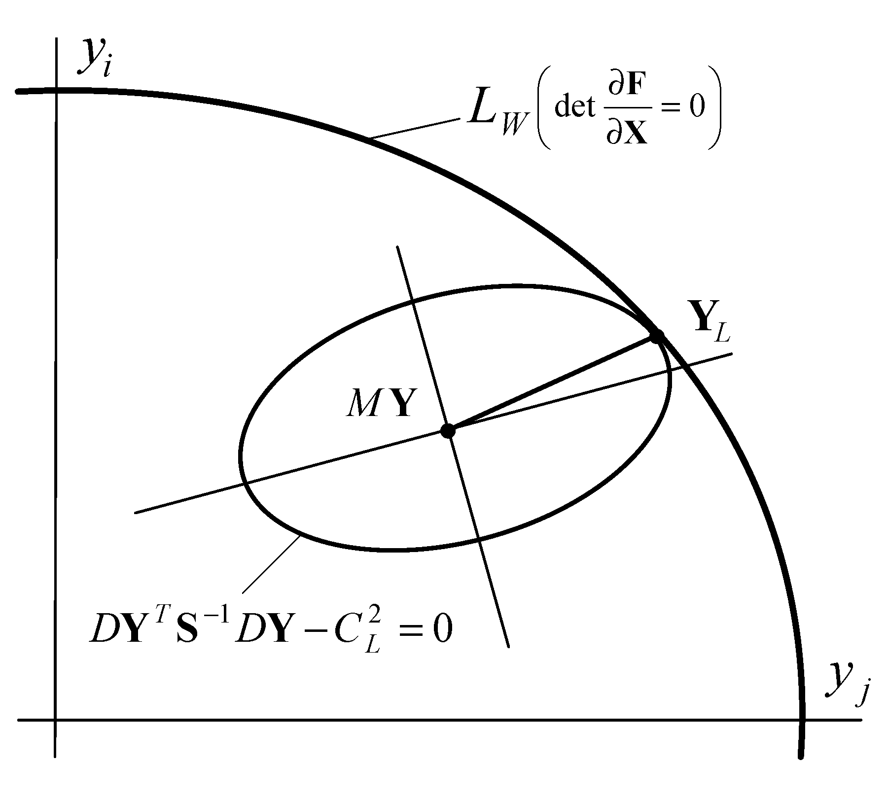
Components of the vector that represent active and reactive powers of generators and loads are random variables. With irregular changes in these parameters, it is possible to reach the boundary ; in this case, reliable operation of the PSS will be ensured if the scattering hyperellipsoid (Figure 1) [4]
With the center at the point does not have common points with the hypersurface . Here ; denotes mathematical expectation; is a covariance matrix; is a value that determines the probability of finding the parameters of Y inside the hyperellipsoid (3). The covariance matrix S participating in (3) can be found using known methods for assessing the state of the PSS [26].
The stochastic approach to assess the margin of SAS can be formulated as follows:
Find
With constraints in the form of the steady-state equations
where F is a nonlinear vector function; X is unregulated operating parameters, which are the magnitudes and phases of nodal voltages or their real and imaginary components.
To solve the problem of minimizing , build a Lagrange function
where is a vector of undefined factors.
The following conditions correspond to the minimum of L:
where is a Jacobian of the steady-state mode equations; is a block diagonal matrix.
It should be taken into consideration that Equation (4) has two solutions:
- The trivial solution corresponds to zero values of the vectors
- The desired solution exists if one or several components of the vectors and are not equal to zero; at the same time, the equations correspond to the condition
Hence, the nontrivial solution corresponds to the hypersurface of the limiting modes.
Equation (4) can written as
Introduce a change of variables
Then, system (4) can be written in the following form
From system (5), we can find a vector
Substituting the resulting value of into the third equation, we can transform the system to the form:
The results of computer simulation show that the iterative process for Equation (6) may converge to a trivial solution. To eliminate this, we can employ the following technique. In system (6), we introduce an additional equation, which corresponds to a nonzero length of the vector , and a variable γ, which ensures the “balancing” of the first vector equation:
A similar technique can be used to improve the efficiency of determining the stability margin in a deterministic statement [3].
Equation (7) is nonlinear and can be solved only by iterative methods, for example, Newton’s method. In this case, the following system of linear equations is solved at each interaction:
Elements of matrix included in this system are determined by the expressions
By differentiating, one can obtain
Hence
where is Hessian matrix of function f1.
If the steady-state equations can have the form
then the following equality is true
where E is an identity matrix. Such a situation occurs when loads are specified by constant power take-offs.
With an implicit Y dependency of X and by using the Cartesian coordinate system, one can write
Or
where , are active and reactive power injections at node i in the initial mode; are active and reactive powers of generators; are active and reactive powers of loads; are real and imaginary components of nodal voltages; is a set magnitude of voltage at the i-th node; , , are components of vector ; are power flows from node i to the network.
To obtain at an implicit X dependency of Y, steady-state conditions should be written in an expanded form:
For generator nodes
For load nodes
where , , , are components of vector ;
are coefficients of polynomials approximating the static characteristics of the load; is rated voltage of the i-th node.
For the nodes corresponding to Equations (8) and (9), matrix will include the following parts:
For generator nodes
| Components of Vector DY | ||
| 0 | ||
| 0 | ||
| 0 |
For load nodes
where = = 1; = ; = .
| Components of Vector DY | ||
| 0 | ||
| 0 |
Based on the value obtained by solving Equation (7), one can calculate that determines probabilistic assessment of the risk of SAS loss; in this case, an approach similar to that proposed in [27] can be used to assess financial risks
where is the value of vector at the point of contact between the hyperellipsoid (3) and the hypersurface LW.
System (7), compared to the steady-state equations that form the first group of equations of this system, has an increased dimension. However, the exclusion of multistep procedures of discrete weighting [10] ensures high efficiency of calculations and reliability of results in the problems of operational control of electric power systems.
4. Simulation Results
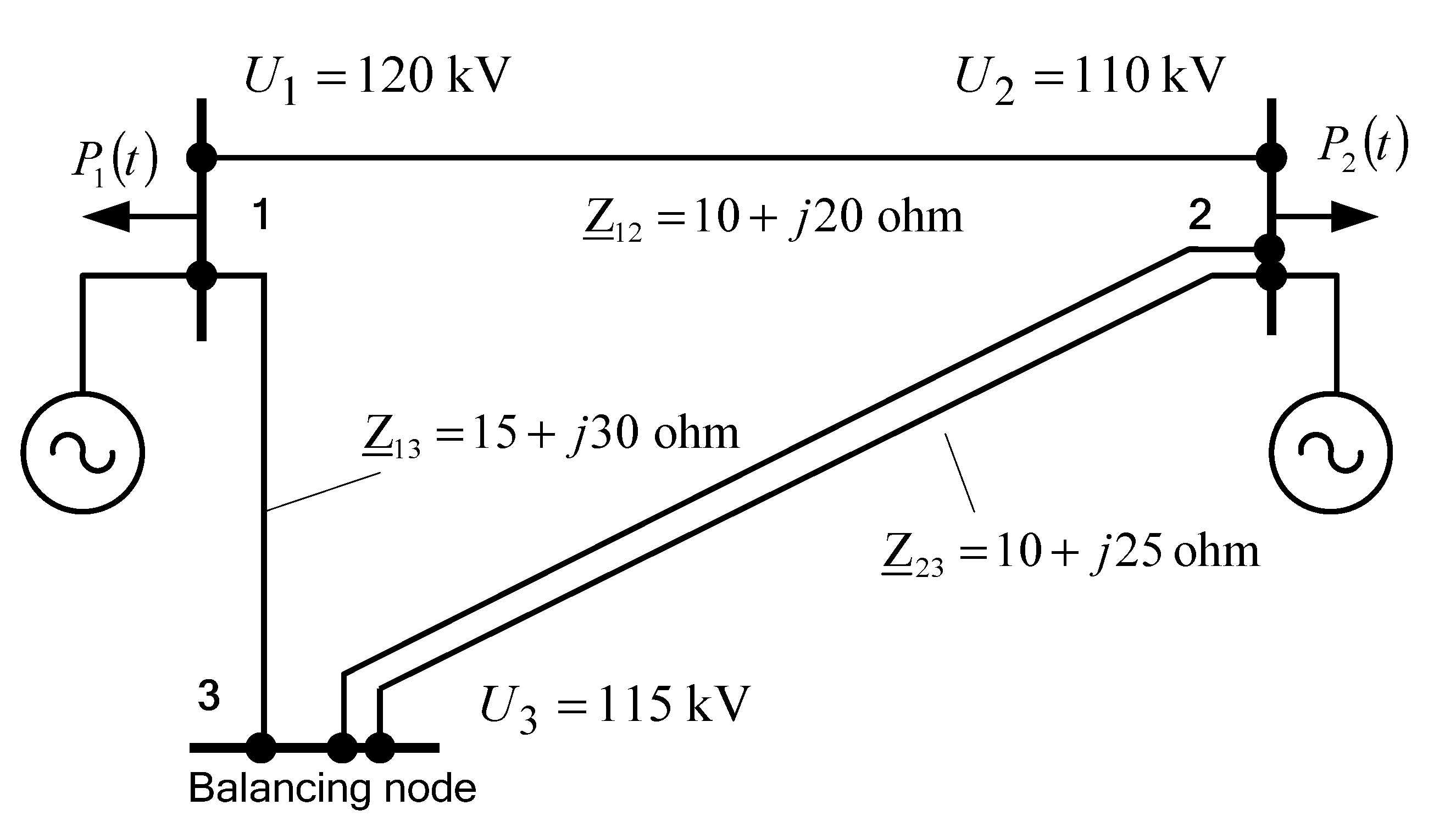
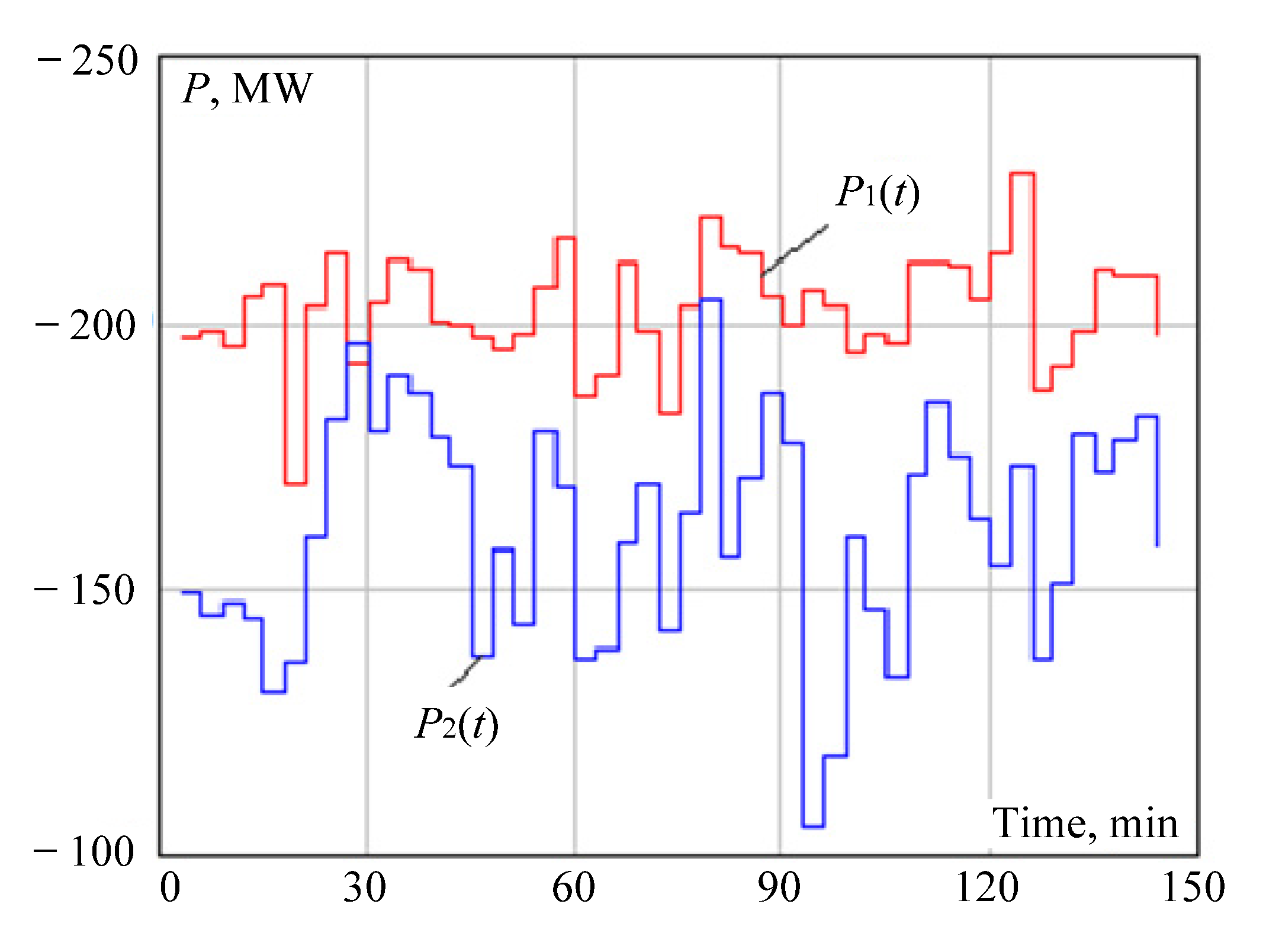
As an example, below are the results of determining the stability margins for a three-node EPS model shown in Figure 2. The model corresponds to a 110 kV network supplying two load nodes equipped with distributed generation (DG) plants with a rated power of 50 MW. Automatic regulators of DG plants provide voltage stabilization on 110 kV busbars. Figure 3 shows the graphs of the power injection changes
where are consumer loads with a random time law; —capacities of generators of the DG plants, which are assumed to be constant; k = 1, 2.
The approach used in this example was based on the following assumptions:
- a stochastic approach was used for consumer loads; at the same time, their capacities changed according to the graphs shown in Figure 2;
- deterministic models traditionally used in practice were employed for the powers of the generator; it should be noted that the algorithm described above can also be used without modifications in the case of a stochastic nature of changes in the capacities of generators.
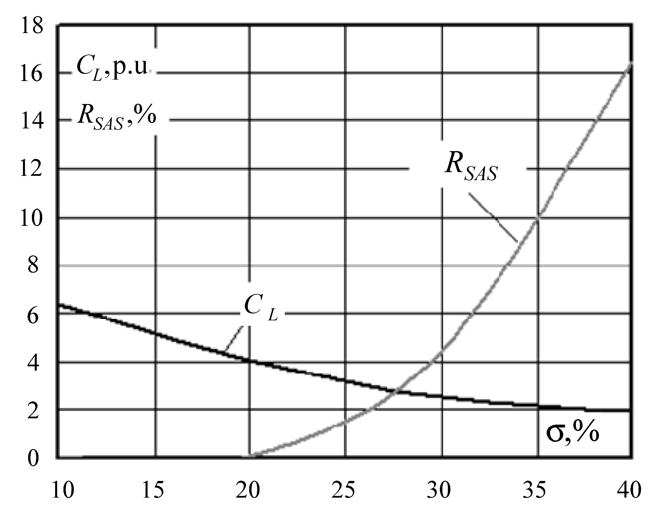
Table 1 presents simulation results obtained on the basis of an experimental code implemented in Mathcad. Figure 4, Figure 5, Figure 6, Figure 7, Figure 8, Figure 9 and Figure 10 provide the corresponding illustrations. Table 1 shows the values of the parameters , characterizing the limiting modes obtained at different values of the standard deviation of the consumer load graphs. In addition, Table 1 provides values of corresponding to hyperellipsoid (3), and the values that determine the probabilistic risk assessments of the SAS loss.
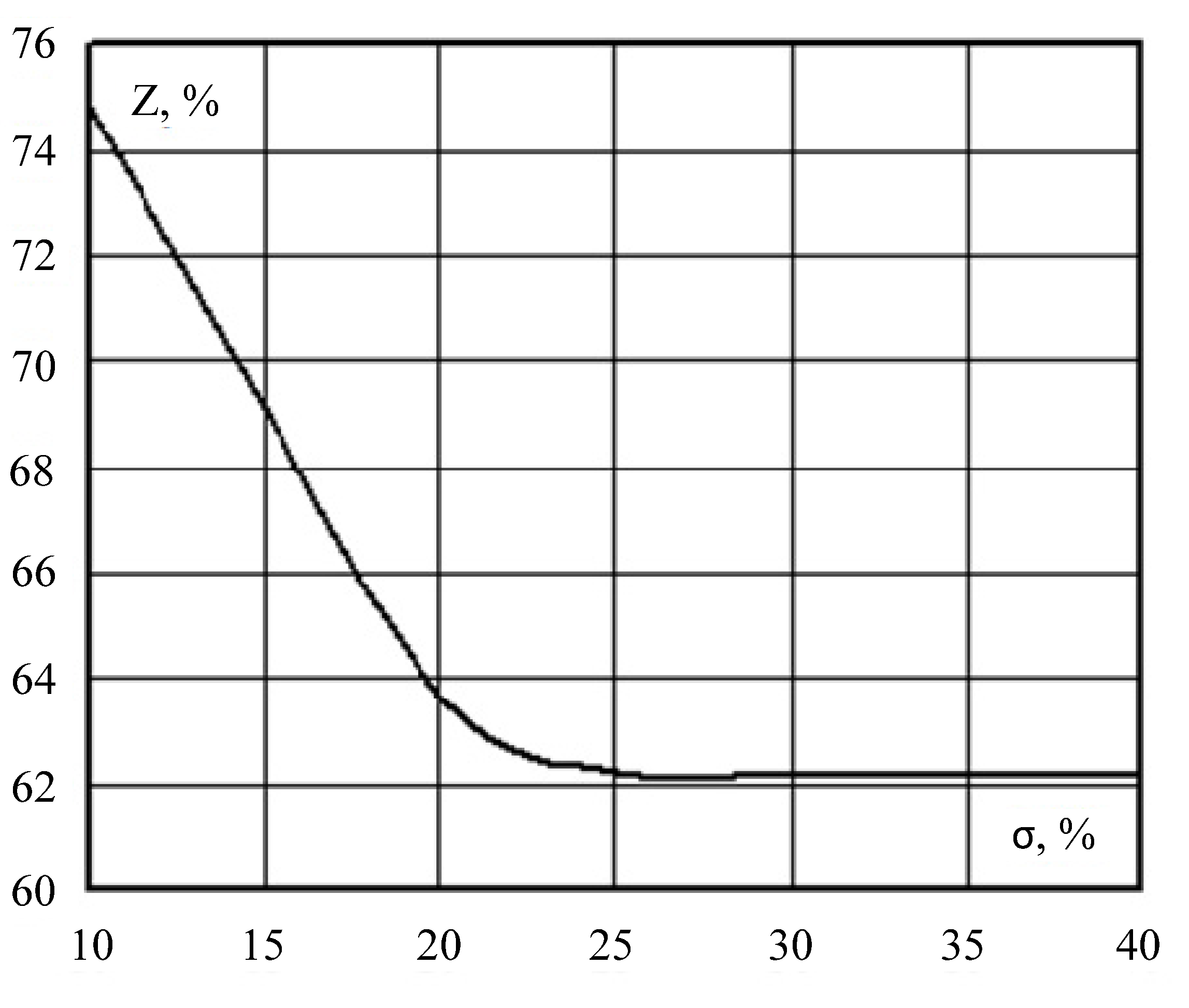
It follows from Table 1 that, with significant load variations, the probability of stability loss can be quite high and reach 16%. However, the stability margin determined by the Euclidean norm (2), which does not take into account the stochastic nature of the operating conditions, will be even higher (62%). Thus, the margin value determined on the basis of the Euclidean norm may be overly optimistic.
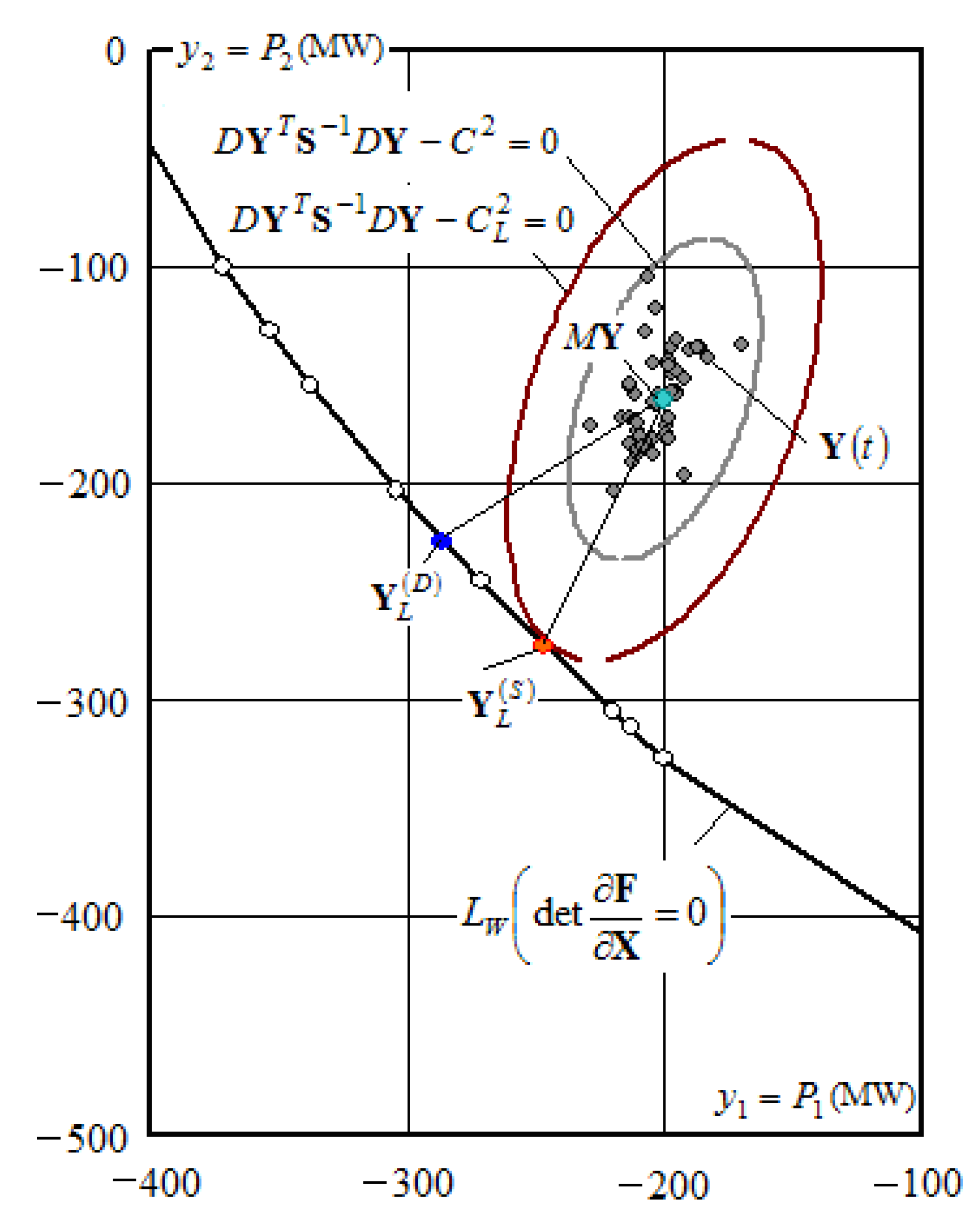
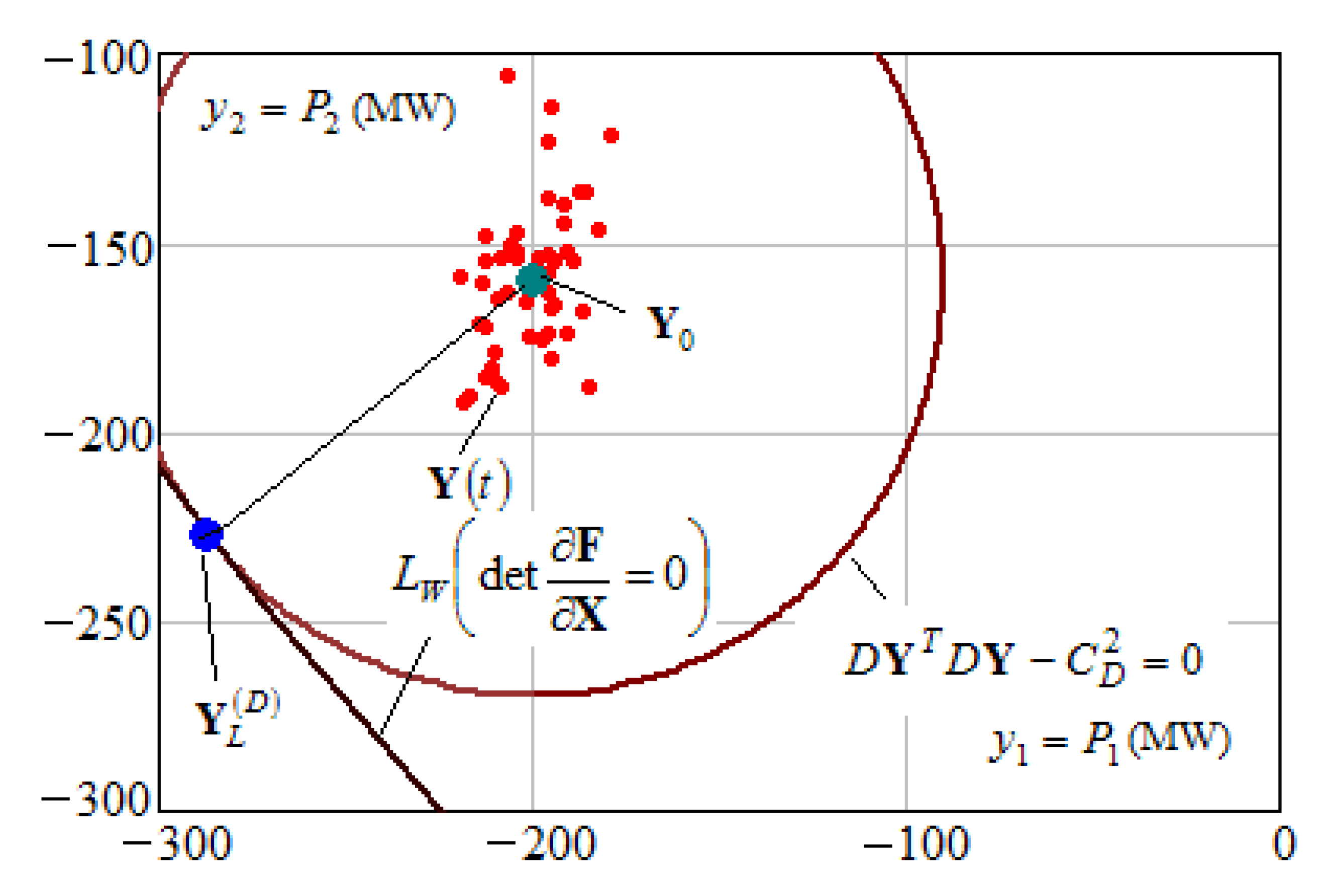
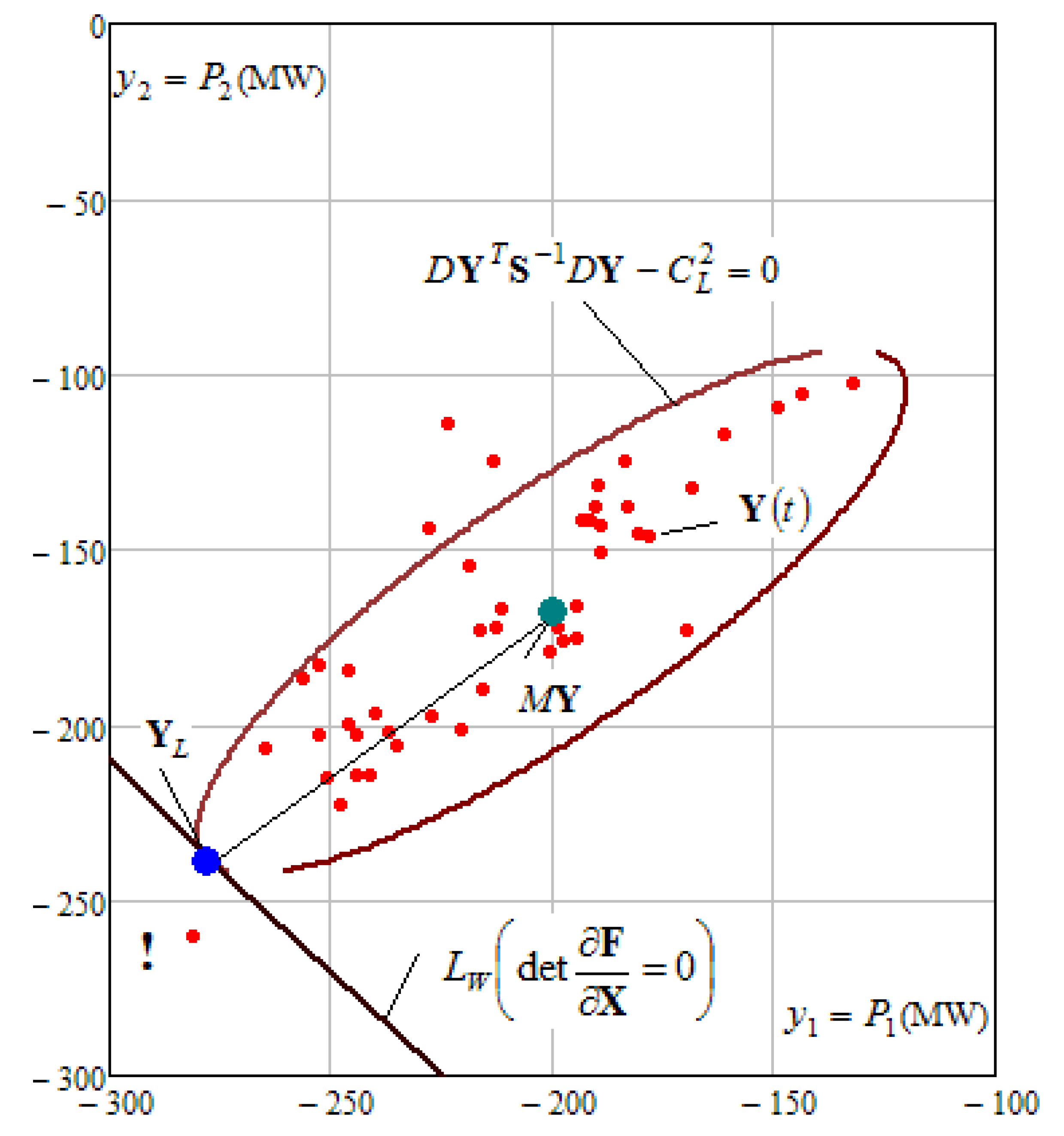
Figure 4 shows the results of determining the limiting modes in a stochastic statement. For comparison, we performed calculation of a limiting mode using a deterministic approach; it was assumed that
where is an identity matrix. The results of calculating the limiting mode in a deterministic statement are illustrated in more detail in Figure 5. As seen in Figure 5, the limiting mode parameters obtained in deterministic and stochastic statements can differ greatly. Figure 6 shows the results of determining the limiting mode for σ = 40%.
Figure 7 shows the results of determining the limiting mode when the 50 MW generator of the DG plant is disabled at node 1. Figure 8 provides illustration for the results obtained when one circuit of the electric transmission line connecting nodes 2 and 3 is disabled.
It should be noted that at the solution to Equation (7), vectors of the normals to the limit hypersurface , subject to
and to hyperellipsoid (3) are collinear.
It was shown in [5] that the vector determined by solving Equation (7) coincides with the direction of the normal to . The direction of the normal to the hyperellipsoid (3) can be found by calculating the gradient vector
Collinearity of vectors and can be determined by finding the angle between them:
Calculations of the limiting mode obtained for = 15% provide the following results:
These results confirm the theoretical findings about collinearity of the vectors R and N.
5. Conclusions
Based on the results of computer simulation, the following conclusions can be made:
- The modified equations that do not allow the iterative process to converge to the trivial solution ensure high reliability of results when determining the stability margins in a stochastic statement; a technique based on the introduction of an additional variable can be used to improve the convergence of computational processes in determining the stability margins in a deterministic statement.
- The parameters of the limiting modes obtained in the deterministic and stochastic formulations may significantly differ.
- With an increase in the variance of load graphs, the risk of stability violation increases significantly; at the same time, the amount of the margin determined on the basis of the Euclidean norm remains overly optimistic.
- In the illustrative example, a significant increase in the risk of stability violation occurs during planned and emergency shutdowns of the EPS components.
- At present, the concept of cyber-physical systems is being actively developed. It provides the foundation for building modern, efficient, and reliable EPSs. This concept presupposes the use of not only physical objects, but also deep integration of digital components that process a large amount of information coming from sensors, which is then used to simulate and control physical objects. The proposed method for determining the stability margins in a stochastic statement can be effectively used to solve the problems of analyzing SAS in cyber-physical EPS equipped with distributed generation units.
- Further research could be aimed at factoring in the asymmetry of loads when determining the stability margins in a stochastic formulation based on the use of phase coordinates to write the equations of limiting modes [28].
Author Contributions
Conceptualization, Y.B., A.K. and K.S.; methodology, Y.B., A.K., V.S. and K.S.; software, A.K.; validation, Y.B., A.K., V.S., K.S. and D.S.; formal analysis, Y.B. and A.K.; investigation, Y.B., A.K., V.S., K.S. and D.S; resources, K.S. and D.S.; data curation, A.K.; writing—original draft preparation, Y.B. and A.K.; writing—review and editing, Y.B., A.K., K.S. and D.S.; visualization, Y.B., A.K. and V.S.; supervision, K.S.; project administration, Y.B. and A.K.; funding acquisition, K.S. All authors have read and agreed to the published version of the manuscript.
Funding
The research was carried out within the state assignment of Ministry of Science and Higher Education of the Russian Federation (project code: FZZS-2020-0039).
Institutional Review Board Statement
Not applicable.
Informed Consent Statement
Not applicable.
Data Availability Statement
Data sharing not applicable. No new data were created or analyzed in this study. Data sharing is not applicable to this article.
Conflicts of Interest
The funders had no role in the design of the study; in the collection, analyses, or interpretation of data; in the writing of the manuscript, or in the decision to publish the results.
References
- Ayuev, B.I.; Davydov, V.V.; Erokhin, P.M. Models of Closest Marginal States of Power Systems in p-Norms. IEEE Trans. Power Syst. 2018, 33, 1195–1208. [Google Scholar] [CrossRef]
- Ayuev, B.I.; Davydov, V.V.; Erokhin, P.M. Fast and reliable method of searching power system marginal states. IEEE Trans. Power Syst. 2016, 31, 4525–4533. [Google Scholar] [CrossRef]
- Kontorovich, A.M.; Kryukov, A.V. The Use of Equations of Limiting Modes in Problems of Power Systems Control; News of the Academy of Sciences of the USSR Power Engineering and Transportation: Moscow, Russia, 1987; pp. 25–33. [Google Scholar]
- Bulatov, Y.N.; Kryukov, A.V. Prevention of Outages in Power Systems with Distributed Generation Plants. Energy Syst. Res. 2019, 2, 68–83. [Google Scholar]
- Makarov, Y.V.; Ma, J.; Dong, Z.Y. Determining Static Stability Boundaries Using A Non-Iterative Method. In Proceedings of the IEEE Power Engineering Society General Meeting, Tampa, FL, USA, 24–28 June 2007; pp. 1–9. [Google Scholar] [CrossRef]
- Vasin, V.P.; Kondakova, V.G. Investigation of the regions of existence of the regime of electric power systems using power series. Izv. RAS Energy 1995, 1, 47–57. [Google Scholar]
- Kirshtein, B.K.; Litvinov, G.L. Analysis of steady-state modes of electric power systems and tropical geometry of the equations of power balances over complex multipoles. Autom. Telemech. 2014, 10, 110–124. [Google Scholar]
- Misrikhanov, M.S.; Ryabchenko, V.N. Methods for the Analysis of Robust Static Stability of Electric Power Systems. In Modern Control Methods for Dynamic Systems; Energoatomizdat: Moscow, Russia, 2003; pp. 483–498. [Google Scholar]
- Bushuev, V.V.; Polyak, A.D.; Pustovitov, V.I. The use of dominant roots to assess static stability margins. Izv. SB AS USSR Ser. Eng. Sci. 1973, 6, 98–104. [Google Scholar]
- Venikov, V.A.; Stroyev, V.A.; Idelchik, V.I.; Vinogradov, A.A. Calculation of the static stability margin of the electrical system. Izv. AS USSR Energy Transp. 1984, 3, 56–65. [Google Scholar]
- Sizhuo, L.; Chao, Z.; Xinfu, S.; Pan, L. Study on the Influence of VSC-HVDC on Receiving Power Grid Voltage Stability Margin and Improvement Measures. In Proceedings of the International Conference on Power System Technology (POWERCON), Guangzhou, China, 6–9 November 2018; pp. 2503–2508. [Google Scholar] [CrossRef]
- Bharati, A.K.; Ajjarapu, V. Investigation of Relevant Distribution System Representation with DG for Voltage Stability Margin Assessment. in IEEE Trans. Power Syst. 2020, 35, 2072–2081. [Google Scholar] [CrossRef]
- Chen, Y.; Mazhari, S.M.; Chung, C.Y.; Faried, S.O.; Pal, B.C. Rotor Angle Stability Prediction of Power Systems with High Wind Power Penetration Using a Stability Index Vector. IEEE Trans. Power Syst. 2020, 35, 4632–4643. [Google Scholar] [CrossRef]
- Saleh, M.S.; Althaibani, A.; Esa, Y.; Mhandi, Y.; Mohamed, A.A. Impact of clustering microgrids on their stability and resilience during blackouts. In Proceedings of the International Conference on Smart Grid and Clean Energy Technologies (ICSGCE), Offenburg, Germany, 20–23 October 2015; pp. 195–200. [Google Scholar]
- Mohsen, F.N.; Amin, M.S.; Hashim, H. Application of smart power grid in developing countries. In Proceedings of the IEEE 7th International Power Engineering and Optimization Conference (PEOCO), Langkawi, Malaysia, 3–4 June 2013. [Google Scholar] [CrossRef]
- Wang, J.; Huang, A.Q.; Sung, W.; Liu, Y.; Baliga, B.J. Smart Grid Technologies. IEEE Ind. Electron. Mag. 2009, 3, 16–23. [Google Scholar] [CrossRef]
- Olivares, D.E.; Mehrizi-Sani, A.; Etemadi, A.H.; Cañizares, C.A.; Iravani, R.; Hajimiragha, A.H.; Gomis-Bellmunt, O.; Saeedifard, M.; Palma-Behnke, R.; Jiménez-Estévez, G.A.; et al. Trends in Microgrid Control. IEEE Trans. Smart Grid 2014, 5, 1905–1919. [Google Scholar] [CrossRef]
- Bulatov, Y.; Kryukov, A.; Suslov, K.; Shamarova, N. Ensuring postemergency modes stability in power supply systems equipped with distributed generation plants. In Proceedings of the 10th International Scientific Symposium on Electrical Power Engineering «Elektroenergetika 2019», Stara Lesna, Slovakia, 16–18 September 2019; pp. 38–42. [Google Scholar]
- Kumar, R.; Singh, R.; Ashfaq, H. Stability enhancement of multi-machine power systems using Ant colony optimization-based static Synchronous Compensator. Comput. Electr. Eng. 2020, 83, 106589. [Google Scholar] [CrossRef]
- Kumar, R.; Diwania, S.; Singh, R.; Ashfaq, H.; Khetrapal, P.; Singh, S. An intelligent Hybrid Wind-PV farm as a static compensator for overall stability and control of multi-machine power system. ISA Trans. 2021, 123, 286–302. [Google Scholar] [CrossRef] [PubMed]
- Sarathkumar, D.; Kavithamani, V.; Velmurugan, S.; Santhakumar, C.; Srinivasan, M.; Semiannual, R. Power system stability enhancement in two machine system by using fuel cell as STATCOM (static synchronous compensator). Mater. Today Proc. 2021, 45, 2130–2138. [Google Scholar] [CrossRef]
- Yang, F.; Ling, Z.; Wei, M.; Mi, T.; Yang, H.; Qiu, R.C. Real-time static voltage stability assessment in large-scale power systems based on spectrum estimation of phasor measurement unit data. Int. J. Electr. Power Energy Syst. 2021, 124, 106196. [Google Scholar] [CrossRef]
- Lombardi, P.; Sokolnikova, T.; Suslov, K.; Voropai, N.; Styczynski, Z. Isolated power system in Russia: A chance for renewable energies? Renew. Energy 2016, 90, 523–541. [Google Scholar] [CrossRef]
- Park, K.J.; Zheng, R.; Liu, X. Cyber-physical Systems: Milestones and Research Challenges. Editor. Comput. Commun. 2012, 36, 1–7. [Google Scholar] [CrossRef]
- Khaitan, S.K.; McCalley, J.D. Design techniques and applications of cyberphysical systems: A survey. IEEE Syst. J. 2014, 9, 350–365. [Google Scholar] [CrossRef]
- Gamm, A.Z. Statistical Methods for Assessing the State of Electric Power Systems; Nauka: Moscow, Russia, 1976. [Google Scholar]
- Pichugin, Y.A.; Malafeev, O.A. On the assessment of the bankruptcy risk of the company. In Proceedings of the International Conference on Dynamical Systems: Stability, Management, Optimization, Minsk, Belarus, 1–5 October 2013. [Google Scholar]
- Zakaryukin, V.P.; Kryukov, A.V. Complicated Asymmetrical Modes of Electrical Systems; Irkutsk State Transport University: Irkutsk, Russia, 2005; p. 273. [Google Scholar]
Figure 1.
Determination of the margin of static aperiodic stability of electric power system in a stochastic statement.
Figure 1.
Determination of the margin of static aperiodic stability of electric power system in a stochastic statement.

Figure 2.
Diagram of an electric power system.

Figure 3.
Load graphs. Following expressions (8) and (9), the sign of the load powers is taken as negative.
Figure 3.
Load graphs. Following expressions (8) and (9), the sign of the load powers is taken as negative.

Figure 4.
Results of determining limiting modes in a stochastic statement.

Figure 5.
Results of determining limiting modes in a deterministic statement: = −287 MW; = −227 MW; = −200 MW; = −161 MW.
Figure 5.
Results of determining limiting modes in a deterministic statement: = −287 MW; = −227 MW; = −200 MW; = −161 MW.

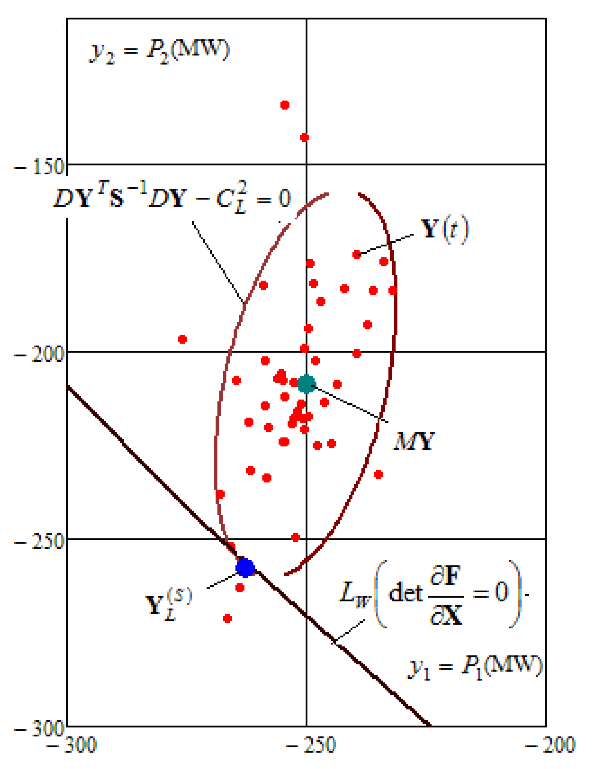
Figure 6.
Increased risk of stability loss with an increase in the load oscillations amplitude (RSAS = 17%).
Figure 6.
Increased risk of stability loss with an increase in the load oscillations amplitude (RSAS = 17%).

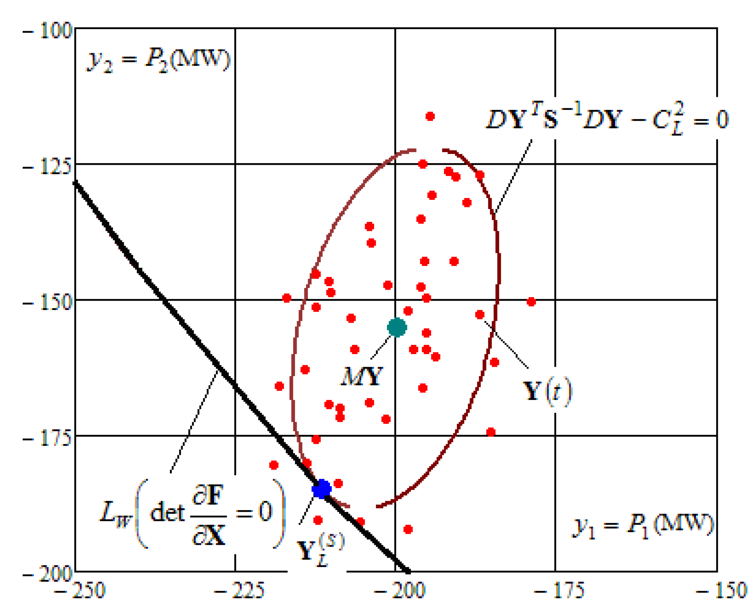
Figure 7.
Increased risk of stability loss with a 50 MW generated disabled at node 1 (RSAS = 14%).

Figure 8.
Increased risk of stability loss with a disabled ETL 2–3 (RSAS = 29%).

Figure 9.
Dependence of the parameter in p.u. and the probability of the mode going beyond the SAS area on the standard deviation of the load capacities.
Figure 9.
Dependence of the parameter in p.u. and the probability of the mode going beyond the SAS area on the standard deviation of the load capacities.

Figure 10.
Dependence of the stability margin on the standard deviation of the load capacities.


Table 1.
Dependence of the parameters of the limiting mode on the standard deviation of the load capacities.
Table 1.
Dependence of the parameters of the limiting mode on the standard deviation of the load capacities.
| Z, % | |||||
|---|---|---|---|---|---|
| 10 | 6.4 | 1.28·10–7 | –248.00 | –275 | 74.76 |
| 20 | 4.03 | 0.03 | –273.00 | –245 | 63.67 |
| 30 | 2.5 | 4.4 | –276.00 | –241 | 62.55 |
| 40 | 1.9 | 16.4 | –278.00 | –239 | 62.19 |
Note: the values of Z were calculated using formula (2).
Publisher’s Note: MDPI stays neutral with regard to jurisdictional claims in published maps and institutional affiliations. |
© 2022 by the authors. Licensee MDPI, Basel, Switzerland. This article is an open access article distributed under the terms and conditions of the Creative Commons Attribution (CC BY) license (https://creativecommons.org/licenses/by/4.0/).
Share and Cite
MDPI and ACS Style
Bulatov, Y.; Kryukov, A.; Senko, V.; Suslov, K.; Sidorov, D. A Stochastic Model for Determining Static Stability Margins in Electric Power Systems. Computation 2022, 10, 67. https://0-doi-org.brum.beds.ac.uk/10.3390/computation10050067
AMA Style
Bulatov Y, Kryukov A, Senko V, Suslov K, Sidorov D. A Stochastic Model for Determining Static Stability Margins in Electric Power Systems. Computation. 2022; 10(5):67. https://0-doi-org.brum.beds.ac.uk/10.3390/computation10050067
Chicago/Turabian StyleBulatov, Yuri, Andrey Kryukov, Vladislav Senko, Konstantin Suslov, and Denis Sidorov. 2022. "A Stochastic Model for Determining Static Stability Margins in Electric Power Systems" Computation 10, no. 5: 67. https://0-doi-org.brum.beds.ac.uk/10.3390/computation10050067
Note that from the first issue of 2016, this journal uses article numbers instead of page numbers. See further details here.