Article

LES: Unsteady Atmospheric Turbulent Layer Inlet. A Precursor Method Application and Its Quality Check †

by
Julien Berthaut-Gerentes
* and
Didier Delaunay
Meteodyn, 14 bd Winston Churchill, 44100 Nantes, France
*
Author to whom correspondence should be addressed.
This work has been presented in the 6th International Symposium on Computational Wind Engineering (CWE 2014, Hamburg, Germany).
Submission received: 24 December 2014 / Accepted: 11 May 2015 / Published: 26 May 2015
(This article belongs to the Special Issue Computational Fluid Dynamics in Civil Engineering)

Abstract

:
The motivation of this work is to bridge the gap between experimental approaches in wind tunnel testing and numerical computations, in the field of structural design against strong winds. This paper focuses on the generation of an unsteady flow field, representative of a natural wind field, but still compatible with Computational Fluid Dynamics inlet requirements. A simple and “naive” procedure is explained, and the results are in good agreement with some international standards.

1. Introduction

Inlet conditions for Large Eddy Simulations (LES) are of the utmost importance, as it determines a large part of the fluid behavior within the computational domain. Tabor and Baba–Ahmadi [1] gave a good overview of the different techniques, classifying them as synthesized turbulence methods and precursor simulation methods.
The first category presents the critical limitation of not achieving a flow field inlet 100% compatible with Computational Fluid Dynamics (CFD) requirements (temporal and spatial fluctuations, divergence-free, spectrum). For instance, the method developed by Jin et al. [2] is not divergence-free. These requirements are of great importance when the purpose of the computations is to generate pressure fields on obstacles. Some regularization methods have to be introduced, as for instance the Synthetic Eddy Method [3].
The second category of techniques is due to Spalart and Leonard [4]. The idea of these methods is to generate inflow condition using CFD itself, as a genuine simulation of turbulence. The inflow of this precursor domain is obtained through a rescaling of the flow field extracted from a downstream location. Nevertheless, even with different stages of simplification [5,6], those techniques are still complicated and not easy to implement. Additionally, they seem more adequate to small turbulence level (Reynolds number Re about 2 × 10³), which does not correspond to structural design against strong winds (Re about 4 × 10⁷).
This paper deals with a more “naive” precursor model. The idea is to draw inspiration from the wind tunnel testing community, with the use of roughness blocks lying on the floor. The large x-axis dimension of the wind tunnel is replaced by a short cyclic domain, in order to convert the large domain issues into a duration matter. Similarly to atmospheric turbulent layer which is driven by geostrophic wind (instead of a horizontal pressure gradient), our flow is naturally driven by the upper boundary condition, acting as a conveyor belt. Re-introducing a flow field extracted downstream becomes straightforward.
The final aim of the method being building dimensioning to high winds, our reference will be an international code concerning these issues: Eurocode I (EN-1991-1-4): “Actions on structures—Wind actions” [7]. This code proposes a systematic approach to describe some of the wind characteristics; we will focus on these characteristics in order to validate—or not—the approach.

2. Description of the Method

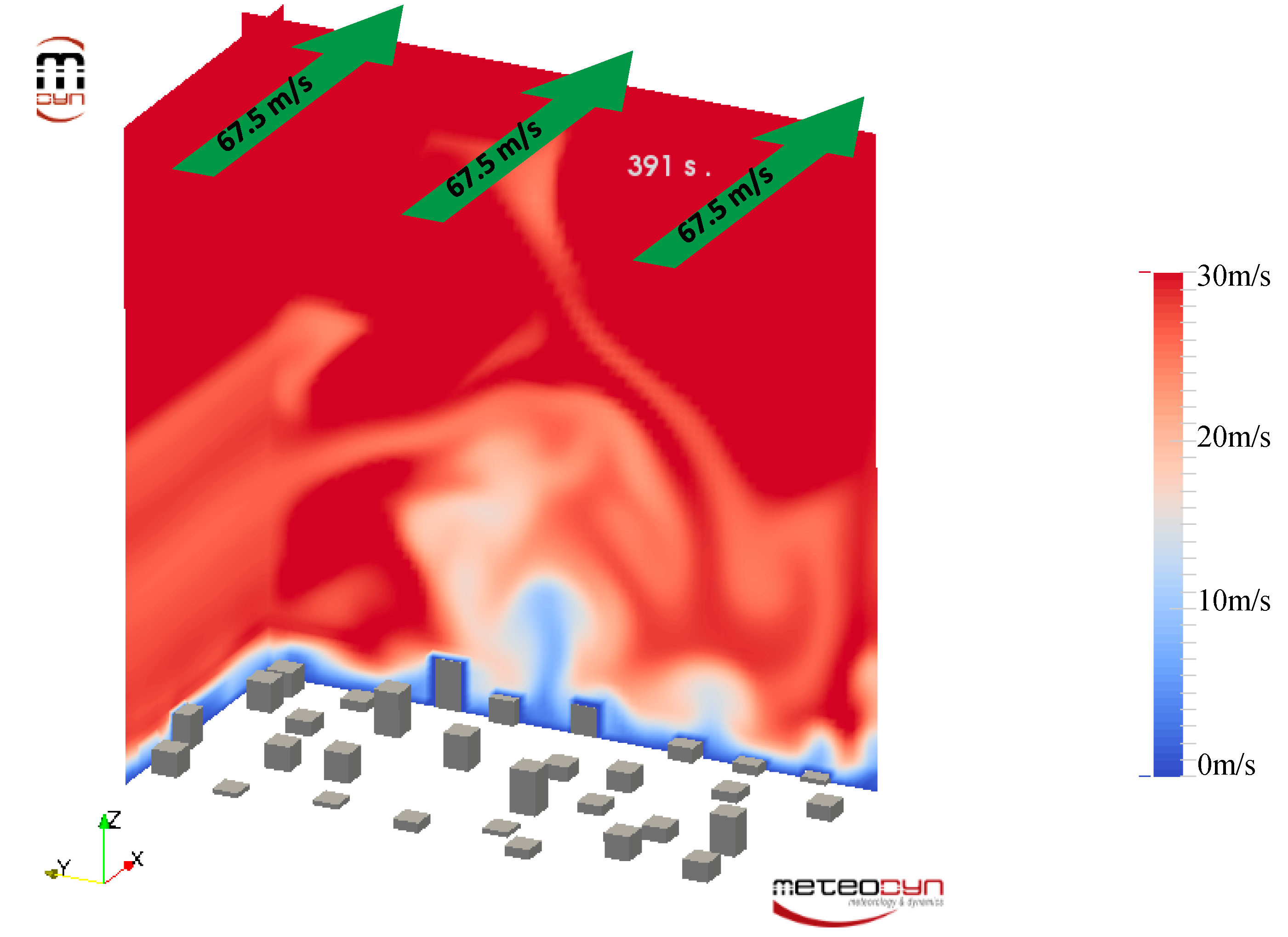
2.1. Aim of the Simulation

In order to compute the extreme loads on a building, CFD calculations have to immerse it in a turbulent atmospheric air flow. Eurocode I (EN-1991-1-4) proposes a systematic and simple approach to describe this air flow: a log-law profile for the mean wind speed, associated with an inverse log-law profile for turbulence intensity.
U ( z ) = V b k r ln ( z z 0 )
I % ( z ) = σ u U = k I ln ( z z 0 )
where U is the 10-min averaged wind speed, z is the height above ground, z 0 is the ground roughness length, V b is the regional base velocity, and k r is a parameter depending only on z 0 . I % is the turbulence intensity, σ u is the standard deviation of the instant velocity (computed on a 10-min window), and k I is a parameter depending only on z 0 .
Wind speeds distributions are Gaussian and the spectrum of turbulence is driven by a modified Kaimal model:
S ( z , v ) = σ u 2 v 6.8   f ( z , v ) ( 1 + 10.2   f ( z , v ) ) 5 3
where S is the single sided power density function, v is the frequency, and f is the reduced frequency:
f ( z , v ) = v   L ( z ) U ( z )
The turbulence scale L is also given by Eurocode:
L ( z ) = 300 ( z 200 ) 0.67 + 0.05 ln ( z 0 )
There is no mention of correlation lengths within the Eurocode. Another regulation, the English code ESDU 75001 [8], gives the correlation lengths in the streamwise direction:
L u x ( z ) = 560 ( z 1000 z 0 0.18 ) 0.35
L v x ( z ) = 280 ( z 1000 z 0 0.18 ) 0.48
L w x ( z ) = 0.7 z
where L u x , L v x and L w x are the streamwise correlation lengths, respectively for the components u (stream wise), v (lateral) and w (vertical).
Our target is to generate an unsteady flow corresponding to this wind model, with a roughness length equal to z 0 = 5 cm and a base velocity equal to V b = 32 m/s. In this case, we have the fallowing values:
  • At 5 m high: L ( 5 ) = 44 m, L u x ( 5 ) = 105 m, L v x ( 5 ) = 28 m, L w x ( 5 ) = 3.5 m
  • At 10 m high: L ( 10 ) = 63 m, L u x ( 10 ) = 135 m, L v x ( 10 ) = 40 m, L w x ( 10 ) = 7 m

2.2. Originality of the Method

The main idea of the method consists of two parts: explicit roughness-cubes on the ground, and short cyclic domain.
In true life, roughness is a succession of obstacles that “sculpt” the air flow and add turbulence. In classic RANS computations, these can be modeled by a statistical approach using some wall functions that describe the mean profiles close to the rough surface. This generates a smooth and uniform flow, with a profile corresponding to the roughness length. However, for LES inlet, it is necessary to describes explicitly the changes in time and space of the wind field: this needs horizontal and vertical strong gradients, which can be generated by some blocks on the floor. The wakes of each element will act as a force opposite to the air flow, and a local turbulence generator. Large scale turbulence will be then explicitly resolved.
A fully developed turbulent layer takes a long span to establish (width δ is O ( X ) and also depends on the roughness length). Thus, to obtain about 20 m-high boundary layer, the domain needs to be several hundred meters streamwise. This would result in a very heavy computation. Nevertheless, from a geometrical point of view, the domain would be similar to it-self; the only difference between a virtual segment of 10 m with its neighbor, would be the inlet. Thus, instead of computing a very long domain, a short domain is preferred with cyclic boundary conditions. However, the segment has to be long enough to integrate several rows of ground cubes. Finally, the initial large domain issues have been converted into a duration matter: the beginning of the simulation will be dedicated to the development of the turbulent boundary layer.

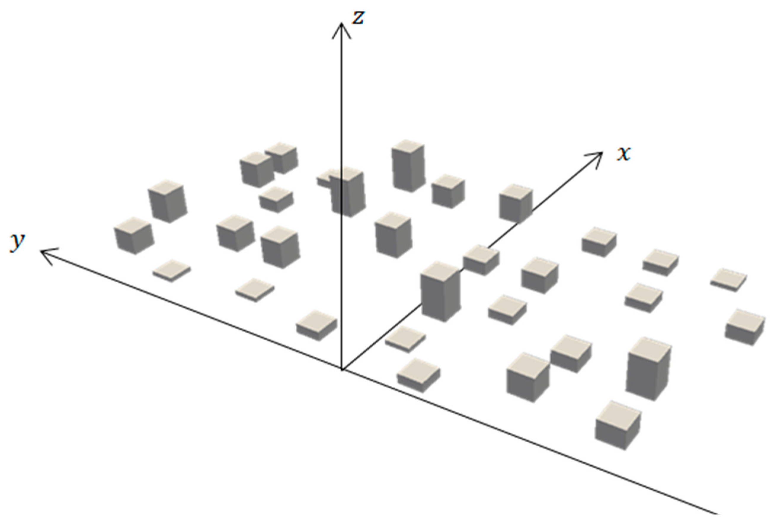
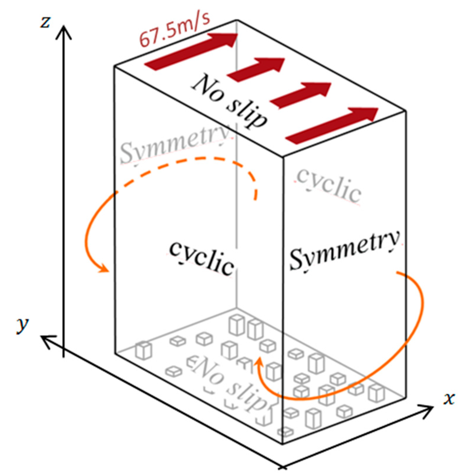
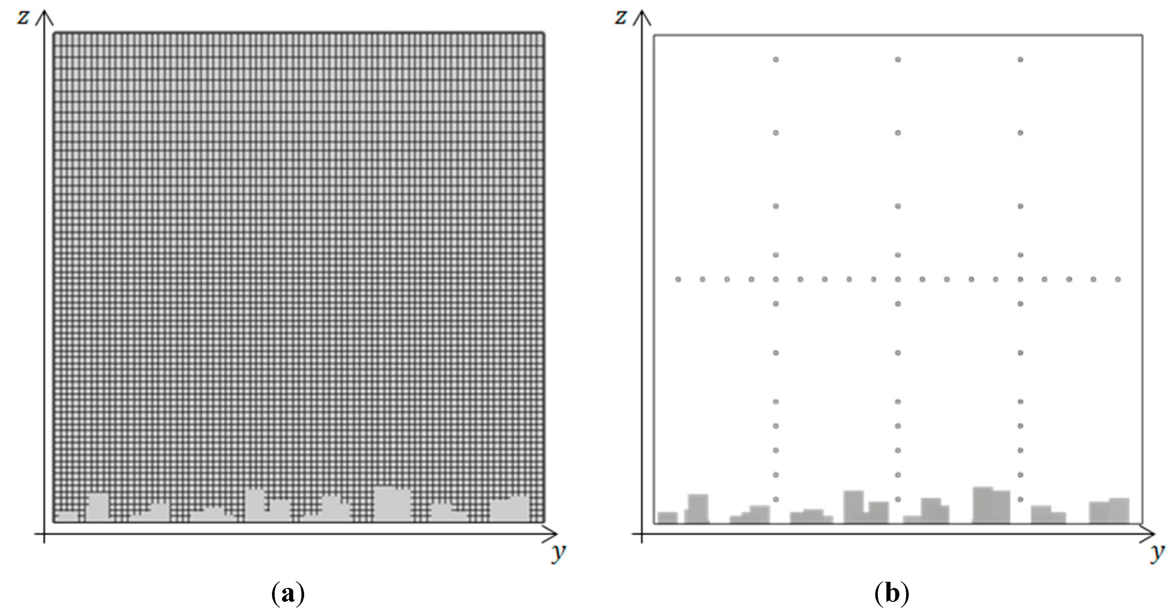
2.3. Geometry and Boundary Conditions

The domain used is a 10 × 20 × 20 m3 box. On the ground, the roughness is modeled by random cubic elements: their size and density are given by some “rule of the thumb” from the experimental wind-tunnel community [9,10]. We start from several cubes sided a = 20 × z 0 (here a = 1   m), with an areal density around 10% (the gap between two consecutive elements is   2 a ). Then some randomness is included: the eight of each block is randomized ( h between 0 × z 0 and 30 ×   z 0 ), as well as its position (each block is allowed to move on its   3 a × 3 a individual panel). Special attention is focused on the lateral homogeneity (the largest cubes should not be grouped on the left or on the right). Figure 1 shows the roughness cubes at the bottom of the computational domain for this study.
Figure 1. Geometry of the roughness-cubes lying on the floor.
Computation 03 00262 g001
No slip Boundary Conditions (BC) are applied on the ground and on the roughness-cubes. Because the cubes are randomly located, a lateral force can appear on the ground. In order to compensate this force and to guide the flow within the x-axis, the lateral boundaries have to block the flow: symmetry boundary condition is chosen on these boundaries. Concerning the inlet and outlet, cyclic BC are used to re-introduce the flow field as it is. The upper-boundary condition is also no-slip on the “roof”, but with a driven wall at 67.5 m/s (67.5 m/s instead of 0 m/s on the ground). This value of 67.5 m/s has been obtained through a try-and-error process: a first calculation, using 40 m/s on this Boundary Condition, gave a base velocity (evaluated as in the Section 3.3) equal to 19 m/s. As the flow is Reynolds quite independent, the results of the simulation may be proportional to this moving roof speed. The final calculation used the roof velocity of 40 × 32 ÷ 19 = 67.5 m/s.
Figure 2 summarizes these boundary conditions.

2.4. Running OpenFOAM

The mesh is a uniform grid (as recommended by A. Passalacqua [11]), with dimensions of 25 cm × 25 cm × 25 cm. In order to slightly reduce the cells number, a pinch of grading is introduced in the upper half space (last upper cell is 50 cm tall, see Figure 3a).
Figure 2. Boundary conditions.
Computation 03 00262 g002
Figure 3. x-projection of computational domain. (a) Meshing and roughness cubes; (b) Probe locations.
Computation 03 00262 g003
This paragraph describes the parametrization used to operate OpenFOAM [12]. The aim is to make people able to reproduce the computation. Pimplefoam is run in order to optimize the time step: maxCo (limit of CFL number) is 10, with a time step close to 4 × 10⁻² s. The time scheme is Crank–Nicholson, the spatial scheme is Gauss Linear (and Gauss LinearUpWindV GradU). The LES is performed with implicit filtering (cubeRootVol with deltaCoeff=1), and subgrid turbulence model is oneEqEddy. The solver for pressure is GAMG, and PBiCG DILU for U and k. The initial condition is to impose a uniform field U equal to 67.5 m/s. Computation has been parallelized on six CPUs using scotch decomposition method. Computation longs about 52 s per time step, which is equivalent to 23 min for one simulated second. The total duration for 600 s is about 10 days.

3. Results

3.1. Spatial and Temporal Extraction Method
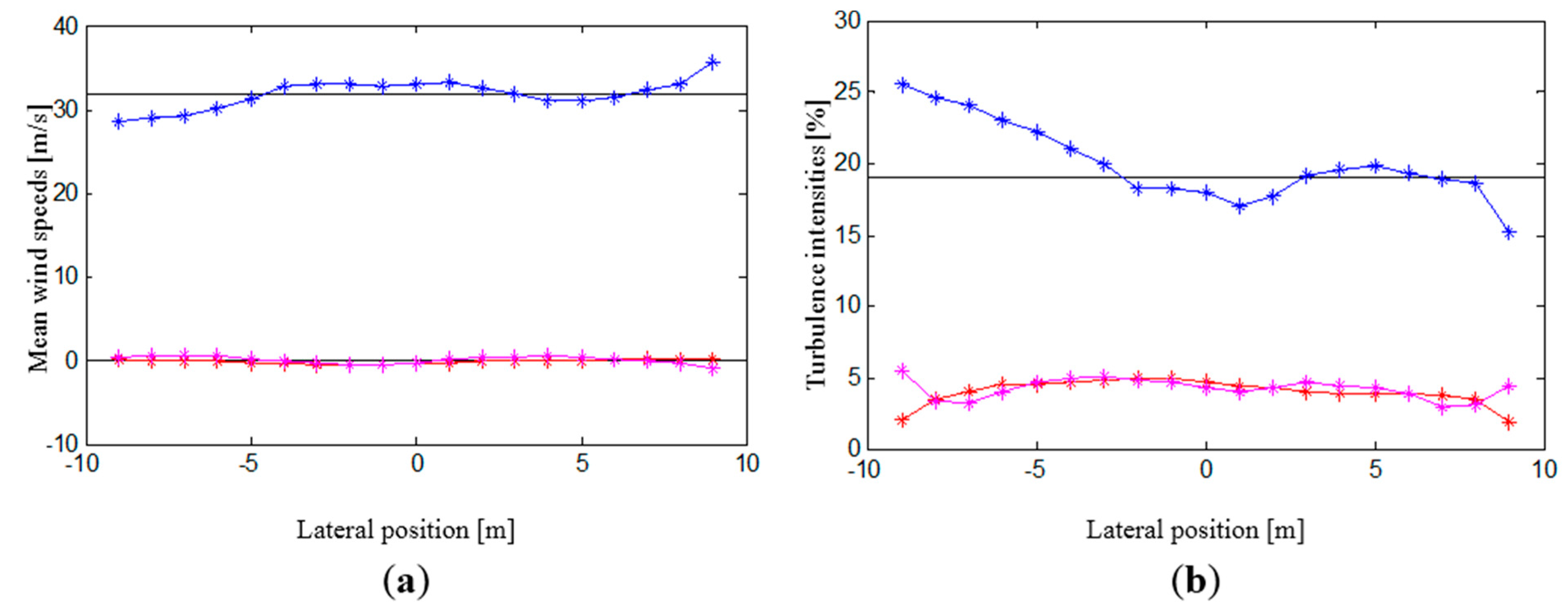
Many probes are placed onto an x-constant plane (1 m close to the outlet), in order to evaluate the success of the method to generate an atmospheric boundary layer: three vertical lines ( y = 0 , center of the domain, and y = ± 5 m, each quarter of domain), to estimate the flow homogeneity and the vertical profiles, and a uniform horizontal line ( z = 10 m, middle of domain) to assess the horizontal homogeneity and correlations (see Figure 3b).
A time span of 300 s is first run. During this first period, the velocity of flow rapidly decreases (from uniform 67.5 m/s), starting to brake from the ground. 300 s turns out to be a good time span in order to achieve a global equilibrium (stationarity). Then the statistics are evaluated over a 300 s window, which is half the meteorological international standard [13].

3.2. First Check

Visual inspection (Figure 4) shows a first validation: the flow field looks like one could expect (heterogeneous, globally the higher the faster, and with some large “structures”. There are no small structures because of the LES filter).
Figure 4. Instant wind field slices in the computational domain.
Computation 03 00262 g004

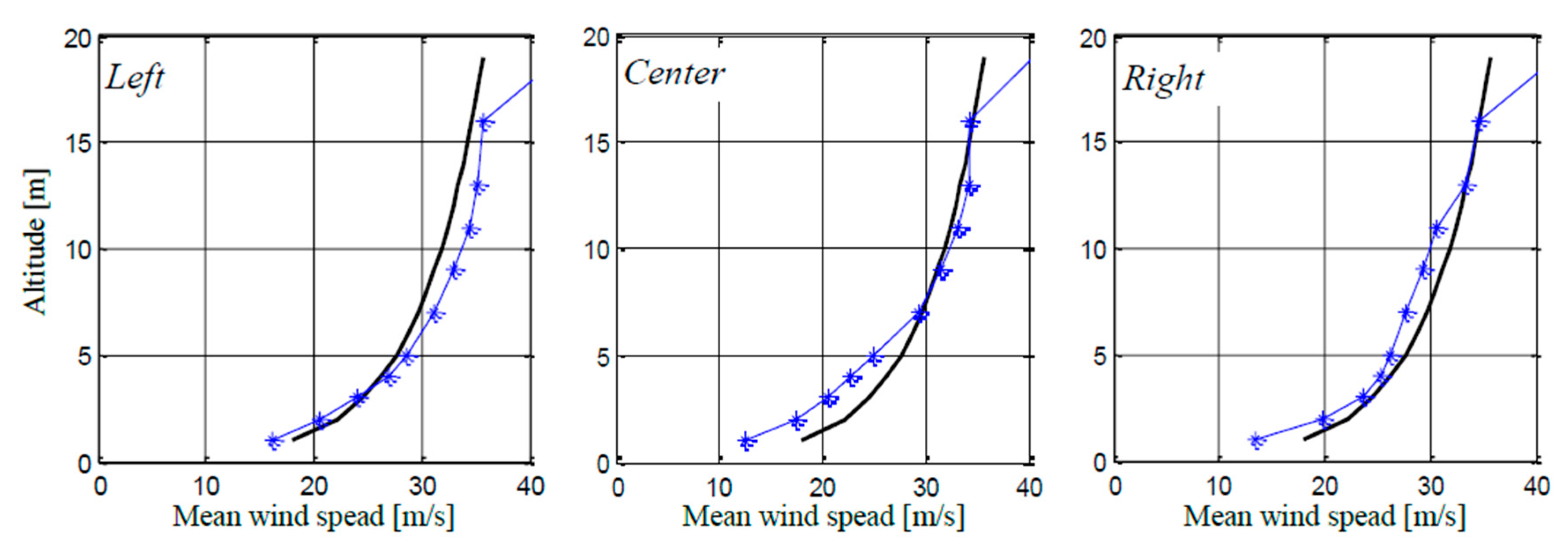
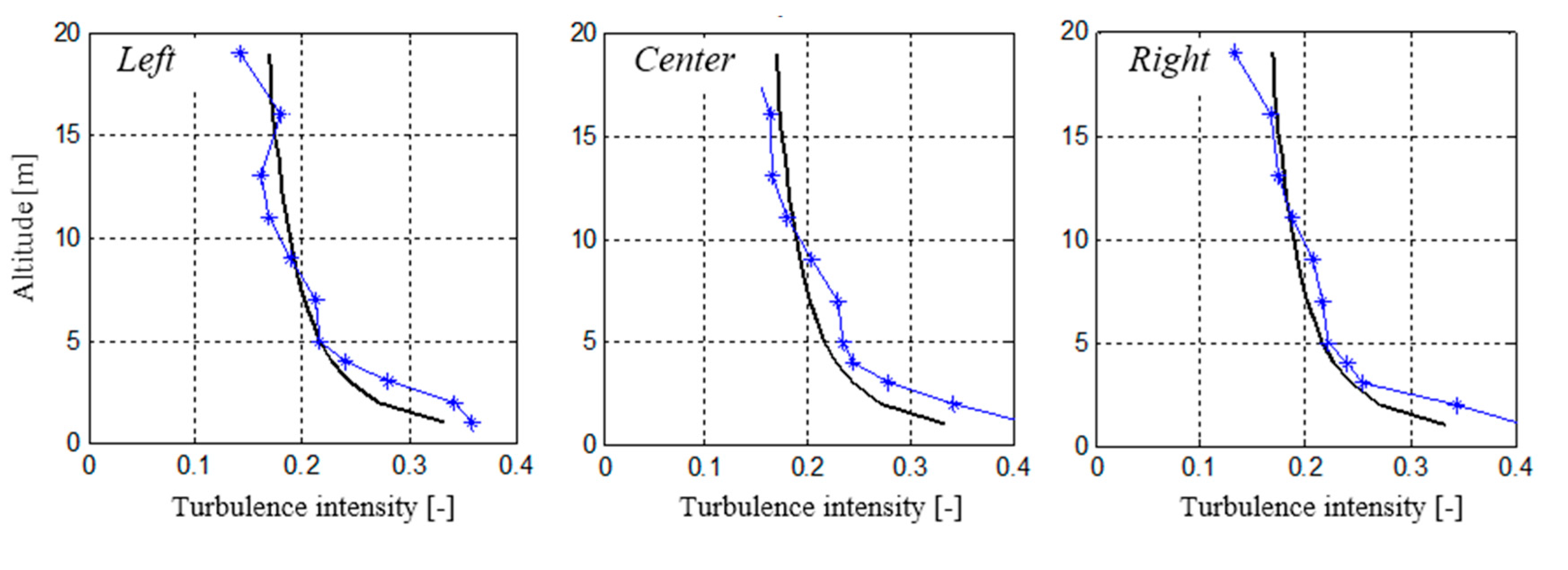
3.3. Results—Comparison with Eurocode

The flow is quite homogeneous: at 10 m high, the mean wind speed and turbulence intensity do not depend on the lateral position (see Figure 5a), at least in the central part of the flow (one half centered span).
Figure 5. Horizontal profile of mean wind speeds (a) and turbulence intensities (b). Blue: u-component, red: v-component; purple: w-component.
Computation 03 00262 g005
At 5 m high, densities are found symmetric, close to Gaussian (Figure 6, bottom). At 16 m high, this is not the case, especially for vertical component ( w , purple points). This might be linked with the proximity of the “roof”; this has to be confirmed in a future work.
Figure 6. Normalized distribution of u (blue), v (red) and w (purple) fluctuating components.
Computation 03 00262 g006
Vertical profiles (mean wind speed, Figure 7, and turbulence intensity, Figure 8) agree very well with the Eurocode model. In those figures, the results from LES are compared with the Eurocode profiles (Equations (1) and (2)), with a roughness length of to z 0 = 5 cm and a based velocity equal to V b = 31.6 m/s. This based velocity is found to be directly proportional to the top boundary condition speed.
Once again, close to the roof (17 m and above), results suffer discrepancy with the free atmospheric boundary layer modeled by Eurocode [7]. The validity of our turbulent wind field is limited to the three fourth of the vertical domain (3/4 H), from the ground.
Figure 7. Vertical profile of mean wind speed. Blue stared: LES results. Black line: Eurocode.
Computation 03 00262 g007
Figure 8. Vertical profile of turbulence intensity. Blue stared: LES results. Black line: Eurocode.
Computation 03 00262 g008
Power density spectra are computed at different locations within the domain. Results are plotted Figure 9 (blue line), as well as Eurocode model (bold black line, Equation (3)). The peak of energy is slightly shifted to low frequencies, corresponding to a turbulence length scale slightly larger than the one proposed by Eurocode (Equation (4)). Nevertheless, the global balance between high and low frequencies is not accurately reproduced: low frequencies are over estimated whereas high frequencies are underestimated. This behavior might be linked with the LES filtering of high frequencies; this has to be confirmed in a future work.
Close to the ground (5 m high), there is a second peak of energy at a reduced frequency around f = 4 . This is the “signature” of the domain size: 10 m long, about 28 m/s, makes a cycling frequency equal to 2.8 Hz, corresponding to a reduced frequency (Equations (3) and (4)) of   2.8 × 44 28 = 4.4 .
This peak of energy is also visible at 10 m high, at a slightly higher frequency, linked with a slightly higher turbulence length ( L U = U X   L U = L X = 63 10 = 6.3 ).
One possibility to push at higher frequency this annoying peak could be to use a shorter domain (e.g., 5 m); this has to be confirmed in a future work.
Figure 9. Power Density Spectra of streamwise component. Blue: LES results. Black line: Eurocode.
Computation 03 00262 g009

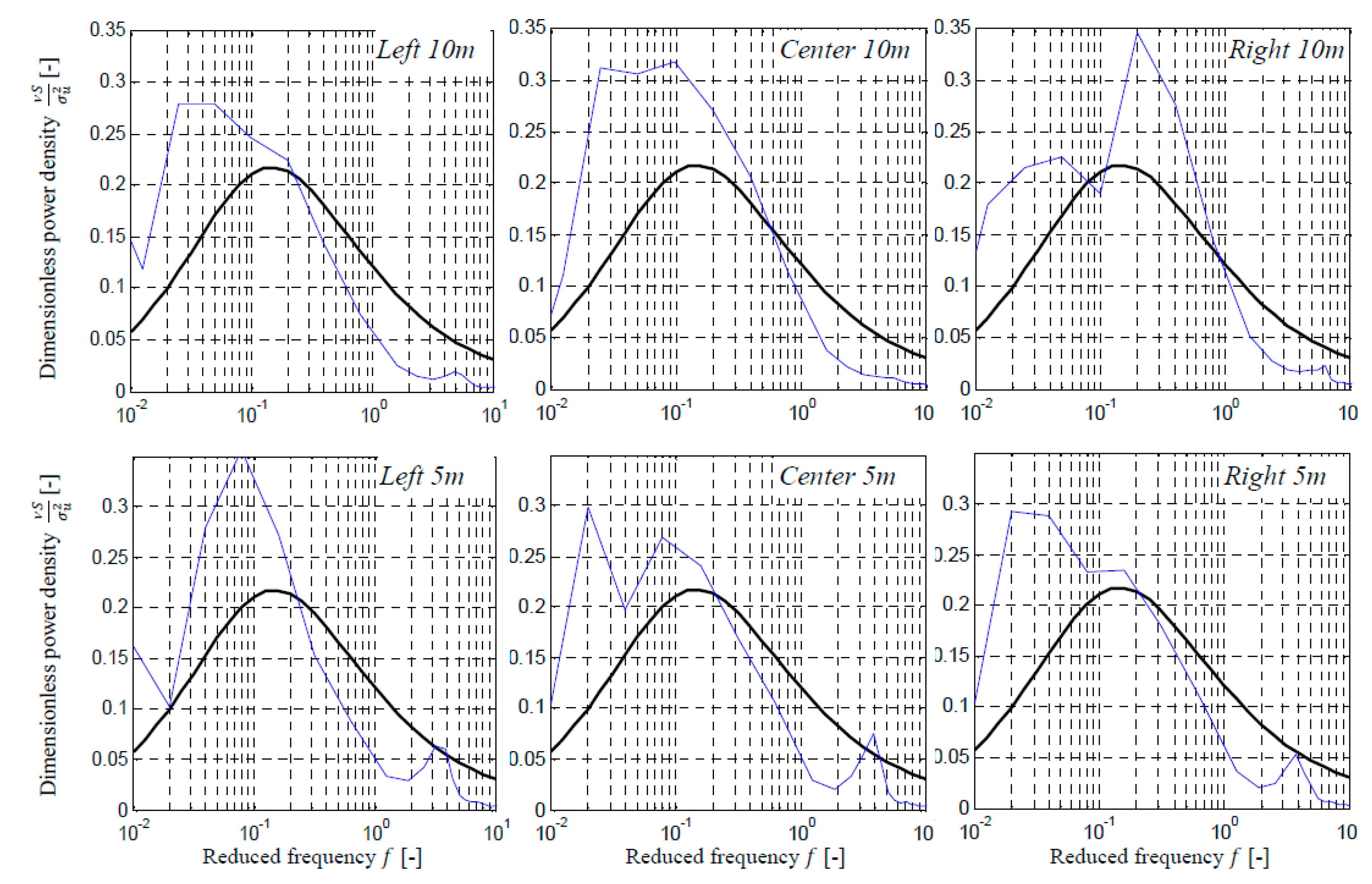
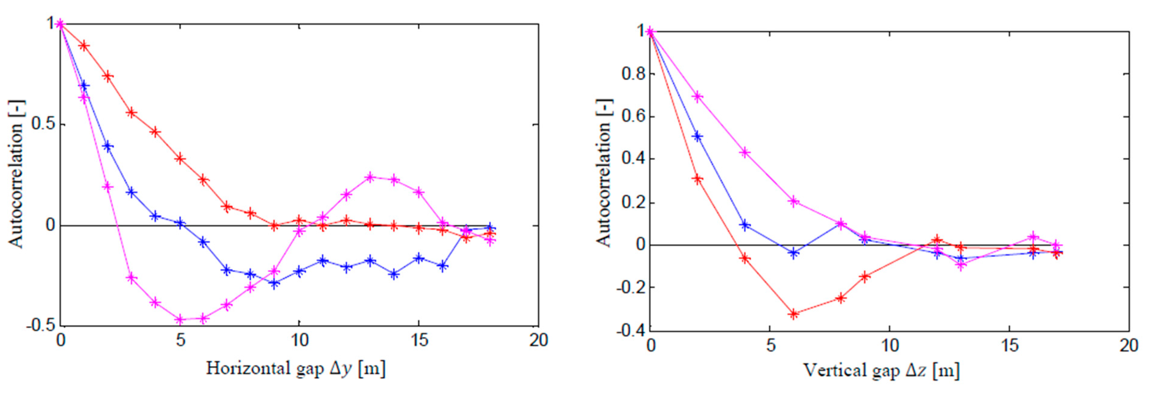
3.4. Correlations—Comparison with ESDU

Streamwise correlation length is evaluated thanks to Taylor’s hypothesis: the temporal correlation (of fluctuating component u, v, and w) is calculated and compared with a negative exponential (Figure 10). The parameter of this negative exponential is given by Formulae (6a) (135 m at 10 m high, 105 m at 5 meter high), divided by the local mean wind speed (given on Figure 7).
Figure 10. Stream wise correlation analysis. Colored lines: LES results. u (blue), v (red) and w (purple). Black line: Eurocode.
Computation 03 00262 g010
The agreement is very good for axial component u , especially at the middle of the domain. For the other two components (v and w), the situation is not so satisfactory: for ESDU, correlation lengths are different for the three axes (Equation (6b) and (6c)), whereas in our LES calculation they appear to be the same.
Through the use of the horizontal array of probes, the lateral correlation can be directly measured. The central vertical array is used for vertical correlation. Results are plotted Figure 11.
Figure 11. Lateral and vertical correlation for the three components. Blue: u-component, red: v-component; purple: w-component.
Computation 03 00262 g011
Lateral and vertical correlation lengths are much smaller than streamwise: we can estimate from Figure 11 around 5 m, which is a quarter of the width and height of the domain. These correlation lengths seem limited by the domain size much more than any other aspect; this assumption has to be confirmed in a future work.

4. Conclusions

A new solution for generating unsteady inlet conditions for Large Eddy Simulation is presented in this paper. This solution, which draws its inspiration from the wind tunnel testing community [14], is as simple as possible and straightforward to implement in OpenFoam. The flow field generated can be directly used as inlet conditions for Large Eddy Simulations.
In the central part of the flow (half centered span laterally, three fourth from ground vertically), the results are compared with international standards concerning wind engineering (Eurocode 1 and ESDU 75001). Densities are found symmetric, close to Gaussian, and the flow is homogeneous (no lateral fluctuations). Vertical profiles of mean wind speed and turbulence intensity fit well with the Eurocode model. The stream-wise correlation length is about 120 m which agrees with ESDU; lateral and vertical correlations are much smaller (about 4~5 m, limited by the computation domain size). The main discrepancies concern the power spectral density: the low frequency domain is a bit over energetic while there is a lack of high frequencies. This misbalance might be linked with the LES filtering of high frequencies.
Future work has to be conducted to verify some assumptions and check the reliability of the method with other characteristics. Authors do not plan to conduct a classic mesh sensitivity-study, because in LES, the physics change with the grid size (implicit filtering [15,16]). What seems important is the ratio between the grid size and the roughness cubes size. Thus, future work will address the problem of changing the roughness length z 0 and the whole domain size.

Acknowledgments

The author greatly acknowledges Alberto Passalacqua for his GeekoCFD live distribution. Thanks also to Bernhard Gschaider for his kind help using swak4foam, and all the CFD online community for their discussions and nice exchanges.

Author Contributions

Julien Berthaut-Gerentes conducted the whole work, under supervision and guidance of Didier Delaunay.

Conflicts of Interest

The authors declare no conflict of interest.

References

  1. Tabor, G.R.; Baba-Ahmadi, M.H. Inlet conditions for large eddy simulation: A review. Comput. Fluids 2010, 39, 553–567. [Google Scholar] [CrossRef]
  2. Jin, S.; Lutes, L.D.; Sarkani, S. Efficient simulation of multidimensional random fields. J. Eng. Mech. 1997, 123, 1082–1089. [Google Scholar] [CrossRef]
  3. Jarrin, N.; Benhamadouche, S.; Laurence, D.; Prosser, R. A synthetic eddy-method for generating inflow conditions for large-eddy simulations. Int. J. Heat Fluid Flow 2006, 27, 585. [Google Scholar] [CrossRef]
  4. Spalart, P.R.; Leonard, A. Direct numerical simulation of equilibrium turbulent boundary layers. In Proceedings of the 5th Symposium on Turbulent Shear Flows, Ithaca, NY, USA, 7–9 August 1985.
  5. Lund, T.S.; Wu, X.; Squires, K.D. Generation of turbulent inflow data for spatially-developing boundary layer simulations. J. Comput. Phys. 1998, 140, 233–258. [Google Scholar] [CrossRef]
  6. Nakayama, H.; Takemi, T.; Nagai, H. Large-eddy simulation of urban boundary-layer flows by generating turbulent inflows from mesoscale meteorological simulations. Atmos. Sci. Lett. 2012, 13, 180–186. [Google Scholar] [CrossRef]
  7. EN 1991-1-4:2005, Eurocode 1: Actions on Structures—Part 1–4: General Actions—Wind Actions. Available online: http://eurocodes.jrc.ec.europa.eu/home.php (accessed on 15 May 2015).
  8. Engineering Sciences Data Unit (1974/1975); ESDU Data Item No. 75001; Characteristics of Atmospheric Turbulence Near the Ground; ESDU: London, UK.
  9. De Bruin, H.A.R.; Moore, C.J. Zero-plane displacement and roughness length for tall vegetation, derived from a simple mass conservation hypothesis. Bound. Layer Met. 1985, 31, 39–49. [Google Scholar] [CrossRef]
  10. Malkawi, A.; Augenbroe, G. Advanced Building Simulation; Routledge: New York, NY, USA, 2004. [Google Scholar]
  11. Passalacqua, A. Comment: “Remember that, strictly speaking, you cannot use a non-uniform mesh in LES, since you assume you can commute the integral and the derivative operators” (2009). Available online: http://www.cfd-online.com/Forums/openfoam-solving/72264-reg-les-openfoam.html#post245231 (accessed on 13 May 2015).
  12. OpenFOAM Foundation—The Open Source CFD Toolbox—User Guide. Available online: http://foam.sourceforge.net/docs/Guides-a4/UserGuide.pdf (accessed on 13 May 2015).
  13. World Meteorological Organization. CIMO Guide, Part I: Measurement of Meteorological VariablesMeasurement of Surface Wind, 2008 ed.; updated in 2010; World Meteorological Organization: Geneva, Switzerland, Chapter 5.
  14. Robert, S. Wind Wizard: Alan G. Davenport and the Art of Wind Engineering; Princeton University Press: Princeton, NJ, USA, 2013. [Google Scholar]
  15. De Villiers, E. The potential of Large Eddy Simulation for the Modelling of Wall Bounded Flows. Ph.D. Thesis, Imperial College of Science, Technology and Medicine, London, UK, July 2006. [Google Scholar]
  16. Top 5 Misunderstandings on (Good) Mesh. Comment: Good mesh is the mesh that serves your project objectives. So, as long as your results are: (1) physical; and (2) accurate enough for your project, your mesh is sufficiently good. Available online: http://caewatch.com/top-5-misunderstandings-on-good-mesh/ (accessed on 13 May 2015).

