Article

On the v-Representabilty Problem in Density Functional Theory: Application to Non-Interacting Systems

Lawrence Livermore National Laboratory, P.O. Box 808, L-372, Livermore, CA 94551, USA
*
Author to whom correspondence should be addressed.
These authors contributed equally to this work.
Submission received: 1 June 2016 / Revised: 28 June 2016 / Accepted: 29 June 2016 / Published: 5 July 2016

Abstract

:
Based on a computational procedure for determining the functional derivative with respect to the density of any antisymmetric N-particle wave function for a non-interacting system that leads to the density, we devise a test as to whether or not a wave function known to lead to a given density corresponds to a solution of a Schrödinger equation for some potential. We examine explicitly the case of non-interacting systems described by Slater determinants. Numerical examples for the cases of a one-dimensional square-well potential with infinite walls and the harmonic oscillator potential illustrate the formalism.

1. Introduction

The Hohenberg–Kohn theorems [1] form the foundation of density functional theory (DFT), on which most ab initio electronic structure methods currently are based. The first theorem proves that the ground state of a many-electron system, described by an external potential, is uniquely determined by the ground state density (within an arbitrary constant). Therefore, the ground state density is the independent variable of DFT. In practice, it is still challenging to find the many-body wave function for the ground state of a potential. That task has been simplified by Kohn and Sham [2], who introduced a non-interacting system (Kohn–Sham system) with the same density as the interacting system that minimized the kinetic energy only. The existence of such a system is only assumed, but essential to the Kohn–Sham formulation of DFT.
In most of today’s applications of DFT, only one direction of the Hohenberg–Kohn theorem is used, to find the ground state density for a given system described by an external potential. For the other direction, the inverse problem, it is a priori not clear if even a potential exists that leads to a given density through the solution of the Schrödinger equation, whether for the interacting or non-interacting system, the problem of v-representability. We refer to the literature [3,4,5,6,7,8,9,10,11] for discussions on the issue of v-representability. Specific examples of v-representable densities as well as non-v-representable densities have been identified.
An alternative formulation of the problem can be developed based on the N-representability property [3,4,5,6] of any density normalized to an integral number of particles, namely that a density can always be obtained from a wave function for a state of N-particles that, for fermions, is antisymmetric with respect to interchange of individual particle coordinates (and spins for electrons). The v-representability problem can be stated as follows: given a density corresponding to a minimizing wave function, as obtained through the constrained search [3], determine whether or not the wave function is derived as the solution of the Schrödinger equation for a system of N electrons, either interacting, or non-interacting. A more general question is concerned with whether or not a wave function that leads to a given density is either interacting or non-interacting v-representable. A formal procedure that addresses this problem for general interacting systems has been published elsewhere [12]. In the following, a density defined with the following properties: it is everywhere non-negative, is normalized to the number of particles, and leads to a finite value of the kinetic energy.
In this work, we focus on the v-representability for non-interacting systems, even though all procedures presented here can be applied for the interacting system in the same way [12]. In previous work [13,14,15], we have derived closed expressions for the functional derivative of terms that only depend indirectly on the density, with respect to it. Using that formalism, we now show analytically that differentiating the non-interacting kinetic energy for a v-representable wave function leads to the negative potential (Kohn–Sham potential), up to a constant. This does not hold for arbitrary wave functions leading to the density. We obtain different wave functions leading to the same density by using a procedure by Cioslowski [16,17], who also showed that each of these wave functions is differentiable with respect to the density. This provides a test establishing whether a given wave function (non-interacting), leading to a density, is non-interacting v-representable. We illustrate these procedures on the one-dimensional particle in a box problem as well as the harmonic oscillator.

2. Results

2.1. Background

The Hamiltonian describing an interacting system of N electrons in an external potential takes the usual form,
H ^ N = V ^ + T ^ N + U ^ N
with the operators V ^ , T ^ N and U ^ N corresponding, respectively, to the external field, the kinetic energy and the inter-particle interaction (Coulomb repulsion for electrons). The ground-state energy of the system is given by the expectation value:
E g = Ψ g N | H ^ N | Ψ g N , Ψ g N | Ψ g N = 1
where Ψ g N denotes the many-particle ground state of H ^ N . We use the notation, Ψ N n ( r ) , and say Ψ N leads to the density n ( r ) , to denote the property:
n ( r ) = N Ψ N ( r , r 2 , , r N ) 2 d r 2 d r N
where n ( r ) denotes the single-particle density function normalized to the total number of particles, N. We now write Equation (2) in the form,
E g = v ( r ) n g ( r ) d r + Ψ g N | T ^ + U ^ | Ψ g N = Min n ( r ) v ( r ) n ( r ) d r + F [ n ] = Min n ( r ) E [ n ]
in terms of the constrained search functional [3,18],
F [ n ] = Min Ψ n ( r ) Ψ | T ^ N + U ^ N | Ψ
Given a density, n ( r ) , the constrained search examines all antisymmetric N-particle wave functions that lead to the density and delivers the state (in the absence of degeneracy) that produces the minimum value of Ψ N | T ^ N + U ^ N | Ψ N .
As in the initial formulation of DFT by Kohn and Sham [2], we postulate the existence of a fictitious non-interacting N-particle system described by the Hamiltonian,
H ^ s N = V ^ s + T ^ N
under the action of an external potential, V ^ s , whose ground-state density is identical to the density of the interacting system described by H ^ N . In analogy with Equation (5), we define the constrained search functional [3],
T s [ n ] = Min Φ N n ( r ) Φ N | T ^ N | Φ N = Φ GS N | T N | Φ GS N = Φ N * ( r ( N ) ) | j 1 2 r j 2 | Φ N ( r ( N ) ) d r ( N )
implying a search over all Slater determinants leading to a given density and returning that determinant that minimizes the expectation value of the kinetic energy for a system of N particles.
Now, assume that the density is non-interacting v-representable for some potential, v s ( r ) , so that from the second theorem of Hohenberg and Kohn [1], it follows that:
δ T s [ n ] δ n ( r ) = v s ( r )
defined within an arbitrary constant. The potential, v s ( r ) , is such that the orbitals entering the construction of Φ N ( r ( N ) ) arise through the solutions of a single-particle Schrödinger equation
1 2 r 2 + v s ( r ) ϕ j ( r ) = ϵ j ϕ j ( r )
with eigenenergies ϵ j . Clearly, the orbitals minimize the expectation value of the kinetic energy, and, as such, form the Slater determinant identified by the constrained search in establishing T s [ n ] . For the case of Slater determinants, Equation (7) reduces to the direct sum:
T s [ n ] = j ϕ j * ( r ) 1 2 r 2 ϕ j ( r ) d r

2.2. Functional Differentiation

The process of performing the functional differentiation of expectation values with respect to the density, however, is not immediately evident: The dependence of a given wave function on the density is implicit, rather than explicitly displayed in terms of the density (or analytic functions of it). This difficulty is resolved through the use of the equidensity orbitals [19,20,21] that are written as explicit functionals of the density and, as shown in [21], form an orthonormal and complete basis in three-dimensional space. This property has been exploited in previous work [13,14,15] to allow the functional differentiation of the Coulomb energy associated with a Slater determinant with respect to the density in order to determine the Coulomb potential including the contribution of the exchange term. A complete discussion is given in [14]. Here, we apply that formalism to derivatives of the non-interacting kinetic energy with respect to the density.
We can obtain the functional derivative of T s [ n ] by differentiating the wave functions under the integral signs in Equation (7), and determine the potential-like quantity,
v s ( r ) = δ T s [ n ] δ n ( r ) = δ Φ N δ n ( r ) | | T ^ N | Φ N + Φ N | T ^ N | | δ Φ N δ n ( r )
where the double bars prohibit the operators from acting on the quantity beyond them. The reason for this is that functional derivatives of wave functions with respect to the density are generally not elements of the Hilbert space. Because of this feature, the operators in the last two equations act on the wave functions, either to their left or their right. It is seen that the combination of the constrained search and functional differentiation allows in principle the determination of all Slater determinants associated with given density that may correspond to a potential.
For the case of a Slater determinant, the last expression takes the form,
δ T s [ n ] δ n ( r ) = j δ ϕ * ( r ) δ n ( r ) 1 2 r 2 ϕ j ( r ) d r + j δ ϕ ( r ) δ n ( r ) 1 2 r 2 ϕ j * ( r ) d r = v s ( r )
where the del operator acts on arguments to its right, and the last line gives the functional derivative as a function of the coordinates that may or may not correspond to a potential. In this expression, the quantity, T s [ n ] , denotes the expectation value of the non-interacting kinetic energy operator, T ^ N , with respect to any wave function that leads to a density.
In previous work [13,14,15], we derived a closed-form expression of the functional derivative of an orbital f ( r ) with respect to the density, δ f ( r ) δ n ( r ) , in terms of ordinary (spatial) derivatives. In the one-dimensional case, excluding terms that would lead to a constant shift in the potential (constants and expressions solely depending on x but not x ), the derivative reads
δ f ( x ) δ n ( x ) = f ( x ) 2 n ( x ) δ ( x x ) + Θ ( x x ) n ( x ) f ( x ) f ( x ) n ( x ) 2 n ( x )
Primes on functions denote spatial derivatives with respect to x, and Θ is the Heaviside step function. Expressions for the three-dimensional case can be found in references [14,15] for both the cases of cartesian and spherical coordinates, respectively.
In Appendix A, we derive an expression for the differentiation of the expression for the kinetic energy (one-dimensional for simplicity) using Equations (12) and (13) (see Equation (A4)). If all orbitals contributing to the kinetic energy originate from the same potential through the Schrödinger or Kohn–Sham equations, we show analytically that the differentiation leads to the negative potential (within an arbitrary constant). The three-dimensional case follows analogously.

2.3. Illustration of the Formalism

The calculations quoted here illustrate the formalism developed above for cases where the potential is given and the wave functions are known analytically. The goal is to reproduce the potential from the functional derivative of the kinetic energy with respect to the density.
For simplicity, we discuss one-dimensional systems in the non-interacting case where the wave function can be represented as a Slater determinant. Analogous procedures will apply in higher dimensions and the interacting framework.
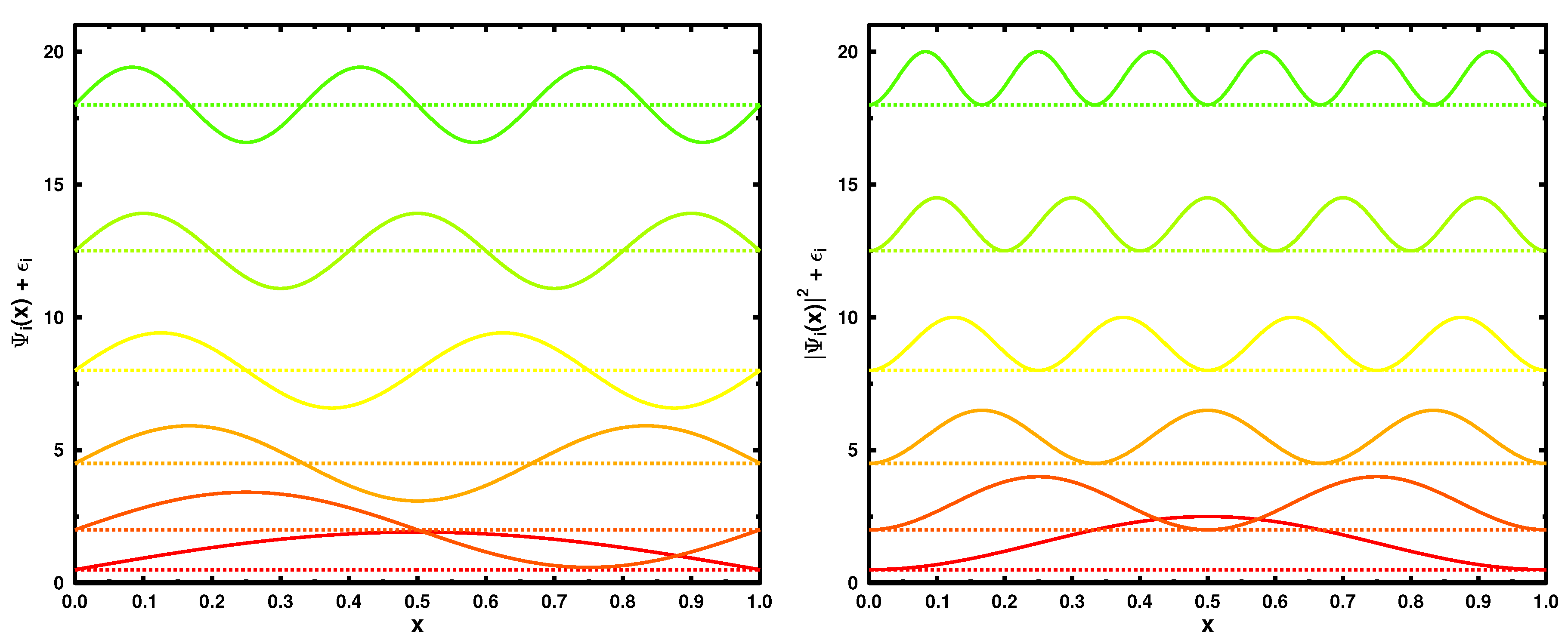
For our first example, we consider N non-interacting particles in a box of length L bounded by potential walls of infinite height. The wave functions of the particles confined in the box are determined through the single-particle Schrödinger equation,
1 2 d 2 d x 2 + v ( x ) ϕ n ( x ) = ϵ n ϕ n ( x )
and vanish at the edges of the box. The ϵ n denote the eigenvalues. When v ( x ) = 0 (or a constant), the normalized single-particle wave functions are given by the expressions,
ϕ n ( x ) = 2 L sin n π x L = A n sin ( k n x ) 0 x L
with quantum numbers n = 1 , 2 , 3 , . The energies take the form,
ϵ n = 2 2 m n π L 2 = 2 2 m k n 2
with the ground state density for a system of N Fermions given by n ( x ) = n = 1 N ϕ n ( x ) 2 . Figure 1 illustrates the six lowest in energy eigenstates (L = 1) (left panel) and their moduli squared (corresponding to single-particle densities) on the right.
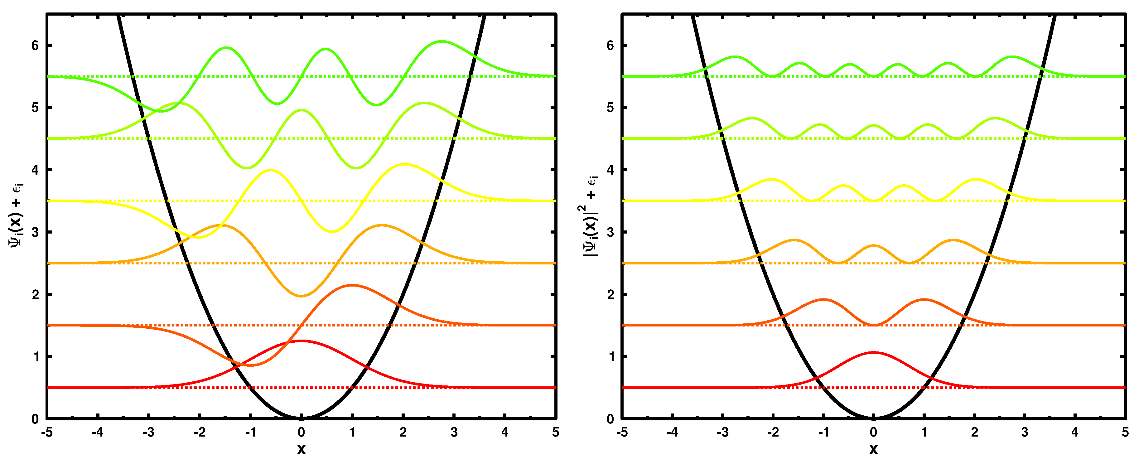
The second example discussed here is the one-dimensional harmonic oscillator. The potential is given by
V ( x ) = 1 2 k x 2 = 1 2 m ω x 2 ω = k m
We make the usual transformation y = α x and α = m ω . The normalized solutions of the Schrödinger equation with the potential (17) read as
Ψ n ( y ) = α π 1 4 1 2 n n ! H n ( y ) e y 2 2
where the H n ( y ) are Hermite polynomials, which are solutions of the differential equations H n ( y ) 2 y H n ( y ) + 2 n y = 0 , and n are integer quantum numbers 0 . The corresponding energies are given by
E n = n + 1 2 ω , n = 0 , 1 , 2 ,
In the following discussion, we set m = ω = = 1 , which corresponds to α = 1 and V ( x ) = 1 2 x 2 . The six lowest in energy single particle wave functions and their corresponding moduli squared are shown in Figure 2.
For both examples, we use Equation (A4) to compute the potential. Since the wave functions are given analytically, the potentials can be calculated analytically. We use Mathematica® [22] to accomplish that task. We tested cases up to N = 6 , and obtained every time the corresponding potential up to a constant. That is not surprising because we have shown in Appendix A that the formalism to calculate those functional derivatives leads to the potential. Equation (A9) also obtains a constant that does not have a physical meaning. Applying l’Hopital’s rule twice at the right boundary for the particles in a box example we obtain the constant:
c = n = 1 N ϵ n n 2 n = 1 N n 2 = π 2 2 L 2 2 m n = 1 N n 4 n = 1 N n 2
Due to the exponential decay of the wave function and the density in the harmonic oscillator example, only the highest in energy of the occupied orbitals contributes to the constant. We find the constant to be equal to the eigenvalue of the highest occupied orbital.
So far, those tests have been performed occupying the lowest N orbitals. We find that any other combination, mimicking a non-ground state, e.g., by occupying orbitals 1 , 2 , 3 , 4 , 5 and 7, also leads to the same potential. The constants for the particles in the box example contains then the sum over occupied orbitals instead a sum from 1 to N, for the harmonic oscillator the constant is still determined by the highest occupied orbital.
The finding that the formalism yields the potential from the kinetic energy is not obvious because the condition δ T s [ n ] δ n ( r ) = v s ( r ) implies the condition of the ground state. On the other hand, those states correspond to a local extremum so that the expression still holds.
Obtaining the potential by a functional differentiation for these examples may sound trivial, but it demonstrates the power of the procedure and the ability to calculate the functional derivative analytically. On the other hand, the procedure can be applied to cases where the the single particle orbitals are given numerically.
So far, we have shown the formalism determines the potential exact (up to a constant) from wave functions by functional differentiation of the kinetic energy, where it is known that all orbitals originate from the same potential, the condition for v-representability. The next step is to determine if a given set of orbitals, forming the density, is v-representable. That can be accomplished by calculating the potential v s ( r ) as shown above, and then checking if each of the orbitals fulfills the Kohn–Sham equation by comparing the right and left-hand sides of the expression:
1 2 r 2 ϕ j ( r ) + v s ( r ) ϕ j ( r ) = α j ϕ j ( ( r ) )
The determinant is v-representable when the equality holds, (for some α j ), for all orbitals forming the determinant. It is convinient for the comparison to normalize the left and right-hand side separately in order to be independent of the α j .
Now, we apply this procedure to the case when the density is given. Generally, the task would be to find the wave function that minimizes the kinetic energy through the procedure of the constrained search [3]. Cioslowski [16,17] has established the formal procedure for generating the complete set of antisymmetric wave functions that lead to a given density. For a Slater determinant, the procedure is outlined in Appendix B. Based on his procedure, for each density, we construct a number of different Slater determinants that leads to it. For each Slater determinant, we differentiate the expectation value of kinetic energy with respect to the the density, obtaining v s ( r ) . Finally, we apply Equation (
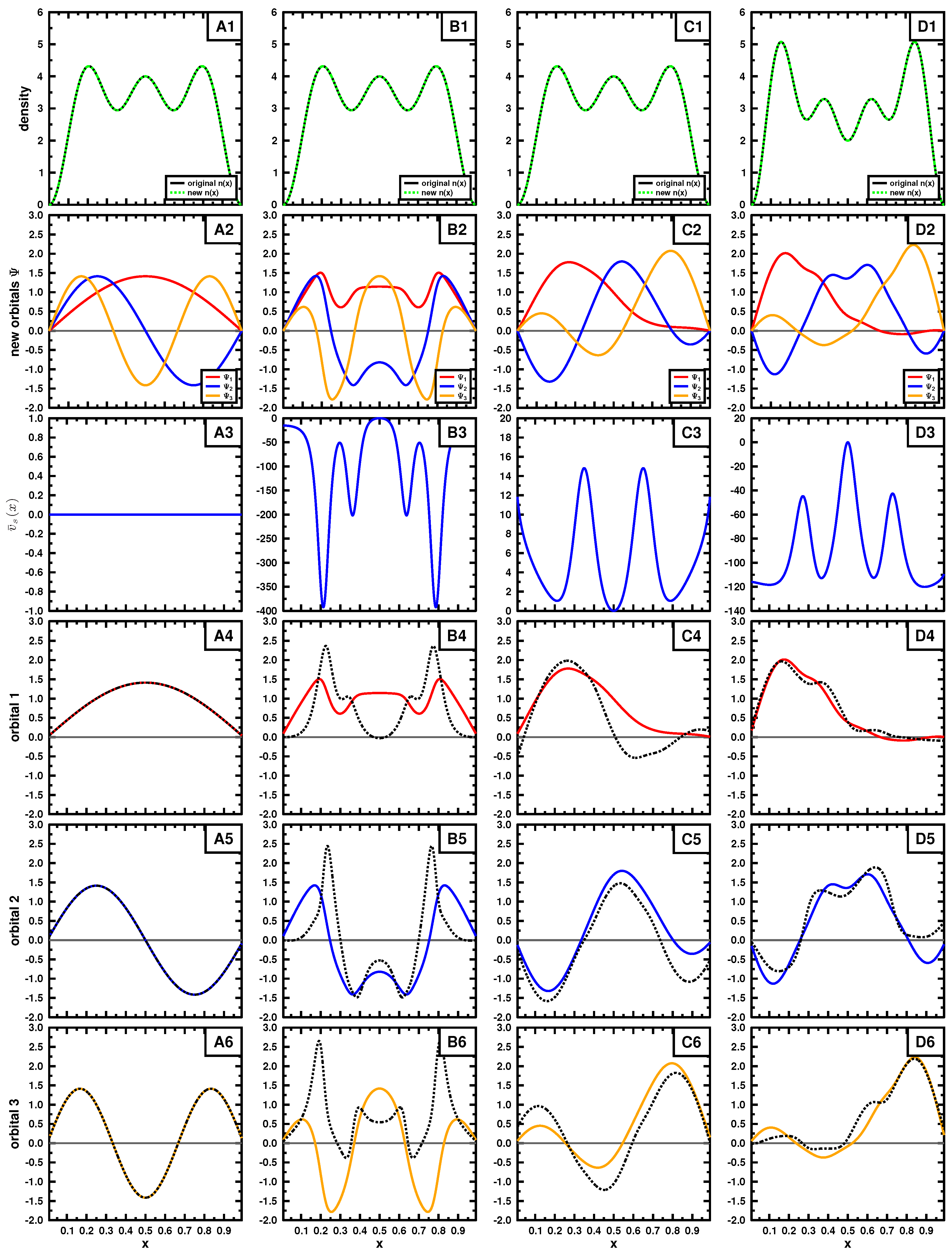
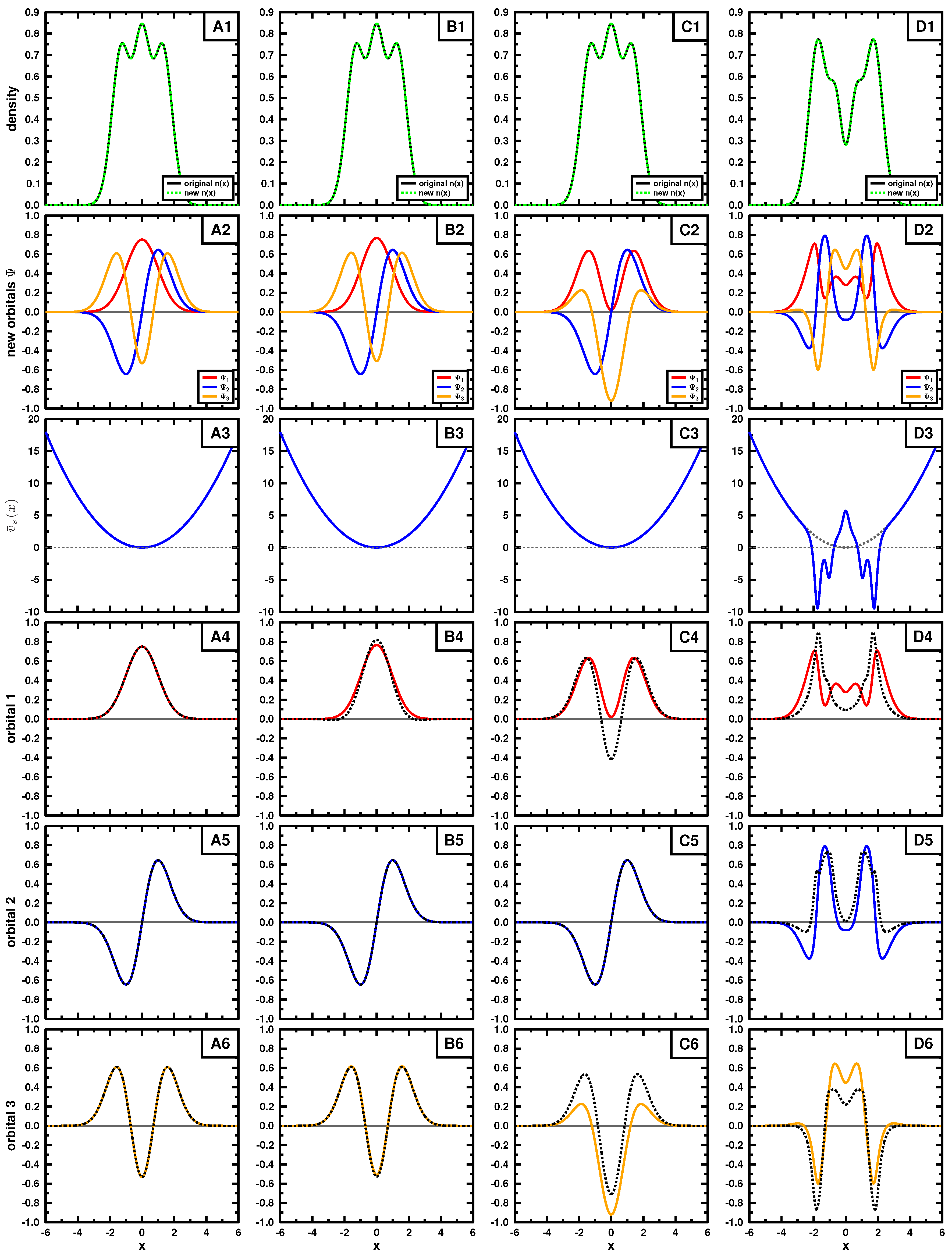
21) for every orbital of the determinant. The results of the test for the case of the particle in the box and harmonic oscillator are shown in Figure 3 and Figure 4, respectively, for a three particle system.
In the figures, the top rows exhibit the density, the second shows the set of three mutually orthonormal orbitals, leading to the density. The third row contains v s , obtained using Equation (A4), for each set of orbitals and the remaining rows compare each of the orbitals with the normalized output corresponding to Equation (21), where, in some, the output is multiplied by 1 .
In both examples, the target density (top row) is obtained using the three lowest in energy orbitals (see Equations (15) and (18); L = 1 ) for panels A,B and C, the density in panel D is constructed by using orbitals 2, 3 and 4. We applied Cioslowski’s procedure [16] for a single Slater determinant using auxiliary functions ϕ given in Table 1 and Table 2 to obtain new Slater determinants leading to the given density. Those new orbitals are shown in the second row. If the exact orbitals are used, Cioslowski’s procedure returns the same orbitals (column A); otherwise, different orbitals are obtained. We note that the auxiliary functions ϕ do not need to be orthogonal or normalized, as long as they are linearly independent. The new orbitals, although mutually orthonormal, can have quite strange forms, as seen in the second row. They do not even have to obey the symmetry of the problem, nor have a specific number of nodes.
Examining these cases, where different sets of orbitals form the same density (columns B and C), we see that the left- and right-hand side of Equation (21) are not the same (see bottom three rows), even though we know the density to be v-representable. This suggests that most of the sets generated by Cioslowski’s procedure [16] may not correspond to a potential, yet all lead to the same density by construction. This behavior is expected from the first theorem of Hohenberg and Kohn: if v-representable, the ground state density determines uniquely the potential and hence the corresponding ground state wave function.
We also applied the procedure to a different density to mimic an exited state (panel D). As seen in panels D4, D5 and D6, the set of obtained wave functions fail to satisfy Equation (21) and hence are not v-representable. The choice of the exact orbitals passes the test of v-representability, as already pointed out above.
In order to quantify the deviation of the left- and right-hand side of Equation (21), the L 2 norm of the difference is shown in Table 3 and Table 4. L 2 norms smaller than the machine epsilon are marked as 0.

3. Conclusions

For a non-interacting system, we have shown how v-representability of a given wave function can be determined. This is accomplished by functional differentiation of the kinetic energy with respect to the density, and checking whether that derivative is a potential leading to the wave function. We have shown analytically (in one dimension), that, in the case of v-representability, the previously derived expressions for the functional derivative of orbitals lead to the correct result, the negative of the potential, when applied to terms depending on the diagonal part of the single-particle density matrix like the expression for the kinetic energy.

Acknowledgments

Comments by Malcolm Stocks and Don Nicholson are gratefully acknowledged. This work was supported by the Critical Materials Institute, an Energy Innovation Hub funded by the U.S. Department of Energy and performed under the auspices of the U.S. Department of Energy by Lawrence Livermore National Laboratory under Contract DE-AC52-07NA27344.

Author Contributions

M.D. derived the analytic proof given in Appendix A, all numerical examples, and also contributed to writing the paper; A.G. contributed to deriving the formalism and writing the paper.

Conflicts of Interest

The authors declare no conflict of interest.

Appendix A. Functional Differentiation of the Kinetic Energy (Non-Interacting)

The non-interacting kinetic energy and its derivative with respect to the density reads (in units = m = 1 )
T s = i f i * ( r ) 2 2 f i ( r ) d r ,
δ T s δ n ( r ) = i f i * ( r ) δ n ( r ) 2 2 f i ( r ) d r + i f i ( r ) δ n ( r ) 2 2 f i * ( r ) d r ,
where f i are solutions of the Kohn–Sham equation, and the sum runs over the lowest in energy states. The last expression can be obtained through twice integrating by parts.
For simplicity, we continue in one dimension. The functional derivative of an orbital with respect to the density reads then, using Equation (13):
δ T s δ n ( x ) = i f i * ( x ) 2 n ( x ) 1 2 f i ( x ) δ ( x x ) d x + i f i ( x ) 2 n ( x ) 1 2 f i * ( x ) δ ( x x ) d x + i x 1 n ( x ) f i * ( x ) f i * ( x ) n ( x ) 2 n ( x ) 1 2 f i ( x ) d x + i x 1 n ( x ) f i ( x ) f i ( x ) n ( x ) 2 n ( x ) 1 2 f i * ( x ) d x
= i f i * ( x ) 2 n ( x ) 1 2 f i ( x ) + i f i ( x ) 2 n ( x ) 1 2 f i * ( x ) + i x f i * ( x ) n ( x ) 1 2 f i ( x ) + f i ( x ) n ( x ) 1 2 f i * ( x ) d x i x f i * ( x ) n ( x ) n ( x ) 2 n ( x ) 1 2 f i ( x ) + f i ( x ) n ( x ) n ( x ) 2 n ( x ) 1 2 f i * ( x ) d x
If the f i correspond to the same potential V and are solutions of a Schrödinger (or Kohn–Sham) equation:
1 2 f i ( x ) = ϵ i V ( x ) f i ( x )
then the expression simplifies to:
δ T s δ n ( x ) = i ϵ i f i * ( x ) f i ( x ) + f i ( x ) f i * ( x ) 2 n ( x ) i f i * ( x ) f i ( x ) 2 n ( x ) + i f i ( x ) f i * ( x ) 2 n ( x ) = 1 V ( x ) + x i ϵ i f i * ( x ) f i ( x ) + f i ( x ) f i * ( x ) n ( x ) d x x i f i * ( x ) f i ( x ) + f i ( x ) f i * ( x ) n ( x ) V ( x ) = n ( x ) n ( x ) V ( x ) d x x n ( x ) 2 n ( x ) n ( x ) i ϵ i f i * ( x ) f i ( x ) + f i ( x ) f i * ( x ) d x + x n ( x ) 2 n ( x ) n ( x ) V ( x ) i f i * ( x ) f i ( x ) + f i ( x ) f i * ( x ) = n ( x ) n ( x ) V ( x ) d x
δ T s δ n ( x ) = V ( x ) + i ϵ i f i * ( x ) f i ( x ) n ( x ) + x i ϵ i f i * ( x ) f i ( x ) n ( x ) d x ,
= V ( x ) + i ϵ i f i * ( x ) f i ( x ) n ( x ) x = = c o n s t ,
δ T s δ n ( x ) = V ( x ) + c
For a finite system, the x = in Equation (A8) signifies the right boundary. To derive Equation (A8), integration by parts is used: a b f [ x ] d x = f [ x ] x = b f [ x ] x = a .

Appendix B. Cioslowski’s Procedure

For a single Slater determinant, we briefly describe how orthogonal orbitals, ψ ( x ) , can be obtained, leading to a given density n ( x ) = i = 1 N ψ i 2 , using Cioslowski’s precedure [16]. From a set of linearly independent auxiliary functions ϕ ( x ) , the ψ i ( x ) are given by the expression:
ψ i ( x ) = f ( x ) i = 1 N s i j ϕ j ( x )
The matrix s ̲ is given by
s ̲ = S ̲ 1 / 2
with
S i j = f ( x ) ϕ i ( x ) ϕ j ( x ) d x
and
f ( x ) = n ( r ) i j ϕ i ( x ) S ̲ 1 i j ϕ j ( x ) 1
The matrix S ̲ exists and has to be obtained self-consistently. That can be accomplished by iterating the equations above, e.g., using an identity matrix as a starting point.

References

  1. Hohenberg, P.; Kohn, W. Inhomogeneous electron gas. Phys. Rev. 1964, 136, B864–B871. [Google Scholar] [CrossRef]
  2. Kohn, W.; Sham, L.J. Self-consistent equations including exchange and correlation effects. Phys. Rev. 1965, 140, A1133–A1138. [Google Scholar] [CrossRef]
  3. Levy, M. Universal variational functionals of electron densities, first-order density matrices, and natural spin-orbitals and solution of the v-representability problem. Proc. Natl. Acad. Sci. USA 1979, 76, 6062–6065. [Google Scholar] [CrossRef] [PubMed]
  4. Levy, M. Electron densities in search of Hamiltonians. Phys. Rev. A 1982, 26, 1200–1208. [Google Scholar] [CrossRef]
  5. Shimony, A.; Feshbach, H. (Eds.) Density functionals for coulomb systems. In Physics as Natural Philosophy: Essays in Honor of Laszlo Tisza on His 75th Birthday; MIT Press: Cambridge, MA, USA, 1982; pp. 111–149.
  6. Dreizler, R.; Providencia, J. (Eds.) Density Functional Methods in Physics; Nato ASI Series B123; Plenum Press: Berlin/Heidelberg, Germany, 1985.
  7. Kohn, W. v-representability and density functional theory. Phys. Rev. Lett. 1983, 51, 1596–1598. [Google Scholar] [CrossRef]
  8. Englisch, H.; Englisch, R. Hohenberg–Kohn theorem and non-v-representable densities. Phys. A Stat. Mech. Appl. 1983, 121, 253–268. [Google Scholar] [CrossRef]
  9. Chen, J.; Stott, M.J. v-representability for noninteracting systems. Phys. Rev. A 1993, 47, 153–160. [Google Scholar] [CrossRef] [PubMed]
  10. Parr, R.G.; Yang, C.Y. Density Functional Theory of Atoms and Molecules; Oxford University Press: Oxford, UK, 1989. [Google Scholar]
  11. Dreitzler, R.M.; Gross, E.K.U. Density Functional Theory; Springer Verlag: Berlin, Germany; New York, NY, USA, 1990. [Google Scholar]
  12. Gonis, A.; Zhang, X.G.; Däne, M.; Stocks, G.; Nicholson, D. Reformulation of density functional theory for N-representable densities and the resolution of the v-representability problem. J. Phys. Chem. Solids 2016, 89, 23–31. [Google Scholar] [CrossRef]
  13. Gonis, A.; Däne, M.; Nicholson, D.; Stocks, G. Computationally simple, analytic, closed form solution of the Coulomb self-interaction problem in Kohn–Sham density functional theory. Solid State Commun. 2012, 152, 771–774. [Google Scholar] [CrossRef]
  14. Däne, M.; Gonis, A.; Nicholson, D.; Stocks, G. On a solution of the self-interaction problem in Kohn–Sham density functional theory. J. Phys. Chem. Solids 2014, 75, 1160–1178. [Google Scholar] [CrossRef]
  15. Däne, M.; Gonis, A.; Nicholson, D.; Stocks, G. Solving the self-interaction problem in Kohn–Sham density functional theory: Application to atoms. J. Phys. Chem. Solids 2015, 79, 55–65. [Google Scholar] [CrossRef]
  16. Cioslowski, J. Density functionals for the energy of electronic systems: Explicit variational construction. Phys. Rev. Lett. 1988, 60, 2141–2143. [Google Scholar] [CrossRef] [PubMed]
  17. Cioslowski, J. Density driven self-consistent field method. II. Construction of all one-particle wavefunctions that are orthonormal and sum up to a given density. Int. J. Quantum Chem. 1989, 36, 255–262. [Google Scholar] [CrossRef]
  18. Lieb, E.H. Density functionals for coulomb systems. In Physics as Natural Philosophy, Essays in Honor of Laszlo Tisza; Shimony, A., Feshbach, H., Eds.; MIT Press: Cambridge, MA, USA, 1982. [Google Scholar]
  19. Macke, W. Zur wellenmechanischen Behandlung von Vielkörperproblemen. Ann. Phys. 1955, 452, 1–9. (In German) [Google Scholar] [CrossRef]
  20. Harriman, J.E. Orthonormal orbitals for the representation of an arbitrary density. Phys. Rev. A 1981, 24, 680–682. [Google Scholar] [CrossRef]
  21. Zumbach, G.; Maschke, K. New approach to the calculation of density functionals. Phys. Rev. A 1983, 28, 544–554. [Google Scholar] [CrossRef]
  22. Mathematica; Version 10.4; Wolfram Research, Inc.: Champaign, IL, USA, 2016.
Figure 1. The six lowest in energy wave functions (left) and the corresponding single particle densities (right) for the particle-in-a-box model (L = 1). For illustrative purposes, all curves are shifted by the corresponding energies (see Equation (16)) in atomic units = m = 1 .
Computation 04 00024 g001
Figure 2. The six lowest in energy wave functions (left) and the corresponding single particle densities (right) for the Harmonic oscillator. All curves are shifted by the corresponding energies (see Equation (19)). The quadratic potential is shown in black.
Computation 04 00024 g002
Figure 3. Results for the square well example, as described in the text. The given density is shown in the top row, where the new orbitals obtained though Cioslowski’s procedure [16] using initial functions from Table 1. The potential, obtained using functional differentiation of the expression of the kinetic energy, is plotted in the third row. The three rows at the bottom show the results of the test (see Equation (21)), where the dashed line corresponds to the left-hand side of the equation, and the solid line to the right-hand side, equal to the new orbital, both normalized. Some of the dashed functions are multiplied by 1 for better comparison, corresponding to a negative α in Equation (21).
Computation 04 00024 g003
Figure 4. Results analogous to those of Figure 3, but for the harmonic oscillator example. New orbitals were obtained through Cioslowski’s procedure [16] using initial functions from Table 2. The dashed line in subfigure D3 shows 1 2 x 2 for comparison.
Computation 04 00024 g004
Table 1. Initial test functions used in Cioslowski’s procedure [16] for the square well example corresponding to Figure 3. The functions in the first row are the exact orbitals (see Equation (15)).
ColumnTest Orbital 1Test Orbital 2Test Orbital 3
A 2 sin ( π x ) 2 sin ( 2 π x ) 2 sin ( 3 π x )
B1 cos ( 2 π x ) cos ( 4 π x )
C1x x 2
D 1 4 + x 1 2 + x 2 3 4 + x 3
Table 2. Initial test functions used in Cioslowski’s procedure [16] for the harmonic oscillator example corresponding to Figure 4. The functions in the first row are the exact orbitals (see Equation (18)).
ColumnTest Orbital 1Test Orbital 2Test Orbital 3
A 1 π 4 e 1 2 x 2 2 π 4 e 1 2 x 2 x 1 2 π 4 e 1 2 x 2 2 x 2 1
B1x x 2
C1 x 6 x 2 18 1
D1 cos π x 6 cos π x 3
Table 3. L 2 norm of the difference of left and right hand side of Equation (21) for the square well example, corresponding to rows 4–6 in Figure 1.
ABCD
orbital 100.51340.25080.0148
orbital 200.77950.18330.1158
orbital 301.90060.16940.0428
Table 4. L 2 norm of the difference of left and right hand side of Equation (21) for the harmonic oscillator example, corresponding to rows 4–6 in Figure 2.
ABCD
orbital 100.013900.236760.33567
orbital 20000.34787
orbital 300.000570.430900.23184

