Numerical Simulation of the Phase Transition Control in a Cylindrical Sample Made of Ferromagnetic Shape Memory Alloy


Institute of Continuous Media Mechanics of the Ural Branch of Russian Academy of Science, 614018 Perm, Russia
*
Author to whom correspondence should be addressed.
Computation 2019, 7(3), 38; https://0-doi-org.brum.beds.ac.uk/10.3390/computation7030038
Submission received: 14 June 2019
/
Revised: 26 July 2019
/
Accepted: 27 July 2019
/
Published: 29 July 2019
(This article belongs to the Section Computational Engineering)
Abstract
:The paper considers ferromagnetic alloys, which exhibit the shape memory effect during phase transition from the high-temperature cubic phase (austenite) to the low-temperature tetragonal phase (martensite) in the ferromagnetic state. In these alloys, significant macroscopic strains are generated during the direct temperature phase transition from the austenitic to the martensitic state, provided that the process proceeds under the action of the applied mechanical stresses. The critical phase transition temperatures in such alloys depend not only on the stress fields, but also on the magnetic field. By changing the magnetic field, it is possible to control the process of phase transition. In this work, within the framework of the finite deformation theory, we develop a model that allows us to describe the process of the control of the direct (austenite-martensite) and reverse (martensite-austenite) phase transitions in ferromagnetic shape memory polycrystalline materials under the action of external force, thermal, and magnetic fields with the aid of the magnetic field. In view of the fact that the magnetic field affects the material deformation, which, in turn, changes the magnetic field, we formulated and solved a coupled boundary value problem. As an example, we considered the problem of a shift of the outer surface of a long hollow cylinder made of ferromagnetic alloy. The numerical implementation of the problem was based on the finite element method using the step-by-step loading procedure. Complete recovery of the strains accumulated during the direct phase transition and reverting of the axially-displaced outer surface of the cylinder to its original position occurred both on heating of the sample to the temperatures of the reverse phase transition and at a constant temperature, when the magnetic field previously applied in the martensitic state was removed.
1. Introduction
Ferromagnetic alloys, which exhibit the shape memory effect (Heusler alloys), belong to the class of functional (smart) materials [1,2,3,4,5,6,7,8,9,10]. The configuration of structures made of such materials can significantly change under the action of external thermal, magnetic, or electric fields. Among a variety of ferromagnetic shape memory alloys, the most studied system is the Ni–Mn–Ga alloy, which is characterized by a structural (martensitic) phase transition from the high-temperature cubic phase (austenite) to the low-temperature tetragonal phase (martensite) in the ferromagnetic state.
There are two different physical mechanisms responsible for the initiation of large deformations (up to 10%) under the action of external forces and magnetic fields. One of them is associated with the rearrangement of structural domains in the martensitic phase and is observed in single-crystal materials or highly-textured polycrystalline samples [1,2,3,4,8]. In the absence of applied mechanical loads, a direct phase transition from a cubic high-temperature phase (austenite) to a tetragonal low-temperature phase (martensite) leads to the formation of twinned martensitic structures (structural domains). In this case, a change in the symmetry of the crystal lattice causes deformations, which, when spatially averaged over a representative volume of a material consisting of a certain number of structural domains, produce only insignificant macroscopic volumetric deformations. The structural domain, in turn, is divided into magnetic domains, in which the magnetization vectors have different directions: in each magnetic domain, this vector is directed along the axis of the easy magnetization of the domain, in which case matching of the domains proceeds in such a way that they minimize the magnetostatic energy. The application of an external magnetic field to ferromagnetic alloys causes the movement of magnetic domain walls, rotation of the magnetization vector, and in the case of high magnetic anisotropy, the martensite reorientation. The first two processes also occur in conventional ferromagnetic materials, while the latter process is inherent only in shape memory alloys: the application of an external magnetic field to the material in the martensitic state (the same as the application of a force field) causes twin boundaries to move in such a way that the axes of easy magnetizations are lined up with a magnetic field induced in the body. The collective reorientation of a certain number of martensitic variants associated with the detwinning of martensitic variants is accompanied by macroscopic deformation, which in some ferromagnetic alloys can be extremely strong. After the removal of the magnetic field, the resulting strains are not recovered, but partially or completely disappear when the material is transformed into the austenitic state in the temperature range of the reverse phase transition.
Another mechanism responsible for the generation of significant macroscopic strains in materials is associated with a direct temperature phase transition from the austenitic state to the martensitic state, when the process proceeds under the applied mechanical stresses. This mechanism operates both in monocrystals and polycrystals [8,9,10]. According to it, the formation of a certain type of the martensitic variant completely depends on the direction of the stress field, which determines the orientation of the resulting strains. The latter are called the phase strains, which add to the normal strains initiated in materials due to application of mechanical forces. The averaging of phase strains over a representative volume of material leads to a macroscopic deformation, which can be much higher than the normal deformation of the material in the martensitic state, but unlike the latter does not disappear after the material is unloaded.
The magnetic field can be used to control the phase transition process effectively, as is evidenced by experimental studies [9,10]. If the direct or reverse phase transitions in a ferromagnetic material are realized under the action of a magnetic field, the critical temperatures of the process are governed by the generalized Clausius–Clapeyron law and depend on the magnetic field and stress fields [11]. Such an effect of the magnetic and stress fields allows one to vary the temperatures of direct and reverse phase transformations and control thereby the process of the austenite-martensite phase transition and vice versa.
In a series of papers [12,13,14], the magnetoelasticity problem (shape memory alloys being excluded) was investigated in the framework of the theory of finite deformations. In a sample of finite size, the internal magnetic field induced by the external magnetic field generates both the mass (ponderomotive) and surface forces in addition to the ordinary, external temperature, or force impacts. In turn, the induced internal magnetic field and the deformation of the sample exert a strong influence on the external magnetic field, causing its disturbances. As a result, the internal field changes, causing variation in the mass and surface forces generated by this field and also in the shape of the sample. In addition, on the surface of a body of finite geometry, the tangential and normal components of the vectors of magnetic induction and magnetic field strength have discontinuities. This gives rise to a surface effect, which manifests itself in a certain region, but is not taken into account in most of the works studying the behavior of ferromagnetic shape memory alloys. Thus, we are faced with the task of solving a coupled magnetomechanical problem for a magnetized body of finite size, which is located in the space exposed to a magnetic field.
To describe the behavior of a ferromagnetic shape memory alloy (FSMA) undergoing direct and reverse phase transformations, it is necessary to develop a physicomechanical model, which will take into account the influence of externally-applied thermal, magnetic, and force fields at different stages of these processes. The model will be constructed using three groups of relations:
- constitutive relations of the solid mechanics;
- relations, describing the direct and reverse, temperature-induced and controlled austenite-martensite phase transitions;
- relations, describing the variation of the magnetic field in a piecewise-homogeneous medium (Maxwell’s equations).
In our work, a variational formulation of a coupled boundary value problem is developed on the basis of these equations. The proposed formulation is used to describe magnetomechanical processes, occurring in a long hollow cylinder made of ferromagnetic material with a fixed inner surface during direct and reverse phase transitions. In such a problem, the magnetic field is homogeneous one and is the same as the externally-applied field when the cylinder is magnetized along its axis. This makes it possible to solve an unconnected magnetic-mechanical problem, in which all variables depend only on the radial coordinate. Such a formulation of the problem considerably simplifies its numerical realization. In the austenitic state, the outer surface of this cylinder is displaced in the axial direction due to a prescribed shear displacement or applied shear force. Then, the cylinder is cooled, which results in a direct phase transition, and the shear forces applied to the outer surface (prescribed or corresponding to the specified axial displacement of this surface) are removed. The cylinder, being currently in the martensitic phase, is under steady-state deformation due to the occurrence of phase strains. After activation of the external magnetic field, the cylinder is heated to the temperature higher than the temperature at the end of the reverse phase transition, which corresponds to the absence of mechanical and magnetic external fields. However, the reverse phase transition does not occur, because the applied magnetic field increases the temperature at which this transition begins. When the magnetic field decreases to zero, the material of the cylinder undergoes a reverse phase transition, and the axially-displaced outer surface of the cylinder returns to its original position.
2. Basic Relations
2.1. Kinematic Relations
In the framework of the finite strain theory, according to [15,16], the problem will be considered in terms of the notions and notation adopted for the examined process: and are the initial (undeformed) and current configurations; is the deformation gradient governing a transfer from the configuration to the configuration; is the measure of the Cauchy–Green strain; is the Cauchy–Green strain tensor; is the metric (unit) tensor. Following [17], we introduce for our consideration the intermediate configuration , which is close to the current configuration and the deformation gradient , which transfers the configuration to the configuration. In this case, the deformation gradient, as well as the measure and tensor of the Cauchy–Green strain for the intermediate configuration, will be given in the following form (see [17]):
In Relation (1), is the gradient of the displacement vector relative to the intermediate state in going from the configuration to the nearest current configuration, is the tensor of a small strain with respect to the intermediate configuration, and is a small positive parameter, characterizing the closeness of the and configurations.
Thus, from Relation (1), in passing to the limit as the intermediate configuration approaches the current one (), we get the following equations:
Here, , and is the strain of displacement rates, coinciding in this case with the rate of strain tensor , .
2.2. State Equation
Out of the equivalent forms of representing the constitutive relations for a simple material, which satisfy the objectivity principle [15,16], we choose the form [17]:
in which is the true stress tensor, is the function of the material response to elastic strain (coincides with the second (symmetric) Piola–Kirchhoff stress tensor: , is the elastic potential), is the third invariant , determining a relative change in the volume, and is the absolute temperature.
From Relation (3), in view of Relation (1), we get the following expression for the second Piola–Kirchhoff stress tensor, which is written for the intermediate configuration accurate for the terms linear in as follows:
Here, and are the forth order tensors determining the response of the material to elastic strain increments and . These tensors are determined in terms of the elastic potential in the following way [17]:
where is the positional scalar left-multiplication (premultiplication) of the second order tensor by the third basis vector of the fourth order tensor [18], and and are specified in the intermediate configuration.
Passing to the limit in Relation (4) yields:
where the tensors and take a form similar to that of the tensors and , but their values are defined in the current rather than intermediate configuration:
3. Phase Transition
The kinematics of the phase transition is described in the framework of the model proposed for shape memory polymers in [19,20,21] and adapted to ferromagnetic shape memory alloys in [22]. We introduce the deformation gradients and to define the elastic strains of the austenitic (A) and martensitic (M) phases. According to (1), we obtain for the intermediate configuration:
Relations (2) are written as:
In view of the additivity of the rates of the variation of elastic (austenitic and martensitic), temperature, and phase strains, the kinematic equation (like in [22]) can be represented in the following form:
where and are the parameters, determining the fraction of the martensitic and austenitic phases in the material volume (), and and are the rates of variation of the phase and temperature strains.
The rate of variation of the temperature strains is specified by generalizing the law of linear temperature expansion to finite deformations:
Here, is the coefficient of temperature expansion.
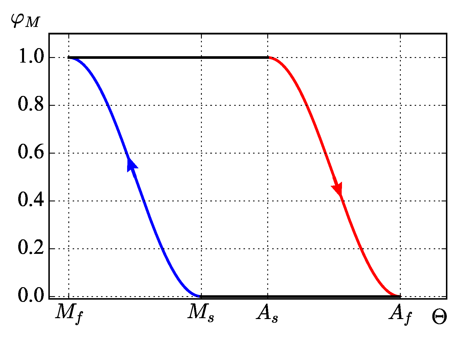
During the direct phase transition, changes from zero (the material is fully austenitic) to one (the material is fully martensitic), during the reverse transition from one to zero. Figure 1 presents a typical diagram of such transitions. Note that the direct and reverse phase transitions occur at different temperatures: the temperature range corresponds to the austenite-martensite transition, and the temperature range corresponds to the martensite-austenite transition.
As an approximation to the dependence of on , we take the expression proposed by A.A.Movchan in [23]:
Here, and are the temperatures at the beginning and at the end of the direct martensitic transformation, and and are the temperatures at the beginning and at the end of the reverse martensitic transformation.
According to [11], the direct and reverse phase transitions are characterized by the temperature , at which the volume fractions of the austenitic and martensitic phases are equal: . As follows from (12) and (13), for the direct martensitic transformation and for the reverse martensitic transformation. In the general case, when the thermal phase transitions occur under the action of stress and magnetic fields, a shift of is governed by the generalized Clausius–Clapeyron law (see [11,22]) during both the martensitic and austenitic phase transitions. In the framework of the theory of finite deformations, this shift is described by the expression [22]:
where is a new value of average temperature, is the value of average temperature in the absence of the stress and magnetic fields, is the vector of the magnetic field strength, , , and are the released (absorbed) heat and changes in the phase strains and magnetization during the phase transition, and is the magnetic constant. Relation (13) in the presence of the stress and magnetic fields is transformed as follows [22]:
where:
and and are the reduced temperatures corresponding to the temperature .
To describe the phase transformation strains, we use the relations proposed in [24], which were generalized in [22] to finite deformations: , where:
Here, are the material parameters, is the deviator of the tensor , and and are the values of the martensitic phase fraction and the phase strains at the initial point of the process of reverse transformation.
In [22], the authors discussed the requirements imposed by thermodynamics on the processes of phase transition in ferromagnetic shape memory alloys. Let us represent the Helmholtz free energy for magnetic materials as the sum of free energies in the austenitic and martensitic phases taken in proportion to their volume fractions, as well as the temperature and magnetic energies . Then, using the Clausius–Duhem inequality, written in the initial configuration as:
in which is the mass density in the initial state, s is the entropy, is the heat flux vector, is the Hamilton operator in the current configuration, and applying the procedure of linear local continuation of the process (see [16]) with respect to the variables , , , and , we arrive at:
where , , .
4. Statement of the Boundary-Value Problem
The internal magnetic field induced by the external magnetic field in a sample of finite size produces a marked effect on the latter causing its disturbances. As a result, the internal field is also transformed. In the absence of electrical currents, changes in the internal and external magnetic fields can be described in terms of the magnetic field vector and the gradient of some scalar function : , where is the applied external magnetic field. The vectors of magnetic induction , magnetic field strength , and magnetization are related by the equation: . From the solenoidal condition of the magnetic field, it follows that . The magnetization law for a material, which is isotropic in the magnetic properties, can be written in a general form as , where is the magnetic susceptibility, . The following relations hold true [22]:
Here, is the volume of the space occupied by the body (sample of finite dimensions) in the current configuration, is the volume of the surrounding medium, is the point in the space, and at .
We assume that the magnetic properties of the representative volume of a material, in which the austenitic and martensitic phases coexist, are determined by averaging over this volume:
where and are the magnetic susceptibility of the martensitic and austenitic phases, which, according to the Froehlich–Kenelly formula [25], can be represented as:
Here, and are the saturation magnetization and the material constant for the martensitic and austenitic phases.
The equilibrium equation accounting for the volumetric magnetic (ponderomotive) forces is written as:
In the magnetic field, the surface of the body is under the action of the following forces:
where , and is the external unit normal to the body surface in the current configuration.
For the FSMA, it is necessary to solve a coupled problem: the magnetic field causes the body to deform, which, in turn, distorts the magnetic field, causing deformation of this body. The variational formulation of the boundary value problem is carried out in the initial configuration , since before developing the problem solution, we lack information on the surface and volume of the body in the current configuration (see [22]). For a body bounded in the initial configuration by the surface and occupying in space the region , the Lagrangian variational formulation of the boundary problem is written as:
where is the external unit normal to the surface of the body in the initial configuration, is the vector of displacements from the initial configuration to the current one, is the vector of volumetric magnetic (ponderomotive) forces, and is the symbol denoting variation.
For the magnetostatic problem, the variational equation in the initial configuration is written as [22,26]:
where ∇ is the Hamilton operator in the initial configuration and is the volume of the surrounding medium of the body in the initial configuration.
To describe the elastic behavior of the austenitic and martensitic phases, we use the simplified Signorini law [15]:
Here, and are the material parameters, which have the meaning of the Lame parameter and the shear modulus of the linear theory of elasticity and is the first principal invariant of the corresponding tensor. For this law, the tensor obtained according to Relation (7) will take the following form:
Here, is the second isotropic tensor of the fourth order [15], is the positional scalar right-multiplication (post-multiplication) of the second order tensor by the second basis vector of the fourth order tensor, while the representation and any similar one correspond to the frequently-used representation , where ⊗ is the tensor product operation [18].
5. Problem Solution
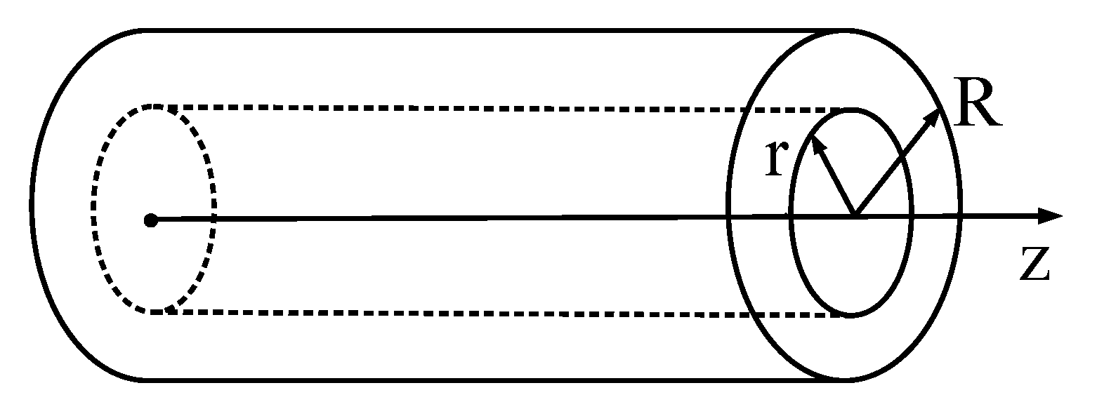
The above relations were used to solve the problem of constricting the outer surface of a long hollow cylinder made of Heusler alloy. At the initial moment of time, a sample of the FSMA in the form of a long hollow cylinder with the inner radius r and the outer radius R is in the austenitic state (Figure 2). The inner surface of the cylinder is fixed, whereas on the outer surface of a constant radius, we prescribed the displacements or the forces , causing its shift relative to the inner surface along the central axis of the cylinder. The cylinder subjected to such deformation is then cooled (with the displacement/force on the outer surface being fixed) to the temperatures characteristic of the direct phase transition, which leads to the accumulation of phase strains. In the martensitic state, the outer surface of the cylinder is unloaded (the forces applied to its surface are removed), so that the configuration of the sample is determined by the accumulated phase strains. A subsequent removal of phase strains in the sample can be accomplished in two ways.
- Heating is performed in the temperature range of the reverse phase transition, and the sample recovers its initial unloaded configuration.
- The sample, which is currently in the martensitic state, is subjected to the external magnetic field and heated to the temperature at which the material would pass to the austenitic state, while not being magnetized. However, the applied magnetic field causes a shift of temperatures in the range of the reverse phase transition temperatures in accordance with the Clausius–Clapeyron law, so that the sample remains in the martensitic state. The reverse phase transition and strain recovery (reshaping) will occur at a constant temperature when the magnetic field is removed. In this process, axial displacement of the cylinder outer surface is not fixed, and the tangential forces on this surface are zero, as noted above.
Note that in the case when the external magnetic field is directed along the axis of an infinitely-long cylinder, the sample is magnetized uniformly. In this case, the magnetic field inside the cylinder is equal to the external magnetic field, .
The problem was solved numerically in the cylindrical coordinates by the finite element method using FEnicCS (http://fenicsproject.org). It was supposed that the nonzero components of the displacement vector depend only on the coordinate , and the temperature distribution over the sample is uniform. The sample was aged for a desired time to achieve such distribution, with the ambient temperature increment being prescribed at each time step.
At all stages of solving the problem, a step-by-step loading procedure was used, for which purpose the variational Equation (17) was linearized. At each step, the increments of the displacement , the force , the temperature , or the external magnetic field were specified such that:
Here, all quantities with a subscript “∗” refer to the intermediate configuration (known quantities at the current step), and the external magnetic field is directed along the cylinder axis .
Numerical calculations were performed using the following parameters of the material [22]: elasticity moduli , ; Poisson’s ratio for the austenitic and martensitic phases ; characteristic temperatures of the phase transition in the absence of stresses and a magnetic field, , , , ; parameters of the material describing the evolution of phase transformation strains , , ; the coefficient of the linear thermal expansion ; magnetic constants , , , .
Below are the results of numerical calculations for a cylinder with the inner radius and the outer radius . Cooling of the sample after a shift of the outer surface in the austenitic state was carried out either at a fixed displacement of the outer surface or under the action of the corresponding force (in the austenitic state). Moreover, , and .
Note that the results obtained at the first stage by solving the problem (only elastic strains in the austenitic state) in the framework of finite deformations are almost consistent with the results of the analytical solution, which can be obtained by solving the problem in the framework of small deformations. For the problem under consideration, the only nonzero component of the displacement vector in the cylindrical coordinate system is the component . In this case, the boundary conditions are written as: , . Using the relations presented in [27,28] and Hooke’s law for relating the stress tensors to the strain tensors , we get:
From the equilibrium equation:
it follows that:
The solution to the derived differential equation is the function , in which the constants and are found from the boundary conditions. As a result, we obtain the following relations: , , , where .
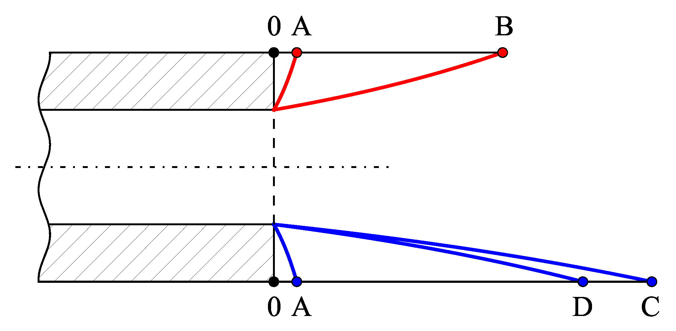
Figure 3 shows the cylinder cross-section and the resulting distributions of the displacements along the radius (multiplied by 100) for the prescribed displacements at the outer surface (shown in the upper part by red lines) and for the prescribed forces (shown in the lower part by blue lines). The elastic solution in the austenitic state corresponds to the O–A path; the A–B path is the result of direct phase transition at a fixed displacement of the outer surface and subsequent complete unloading of this surface in the martensitic state; the B–O path corresponds to the reverse phase transition. The A–C path is obtained after the direct phase transition under a fixed force applied to the outer surface, while subsequent complete unloading of this surface in the martensitic state results in the C–D path. The D–O path is associated with the reverse phase transition.
The axial displacement of the outer surface of the cylinder in the unloaded martensitic state (points B and D) is 10-times greater compared to the prescribed displacement (points A) in the transition at a fixed axial displacement and 13.5-times greater in the transition under a fixed axial force due to the occurrence of phase transformation strains, which still persist in the martensitic state after removal of the force.
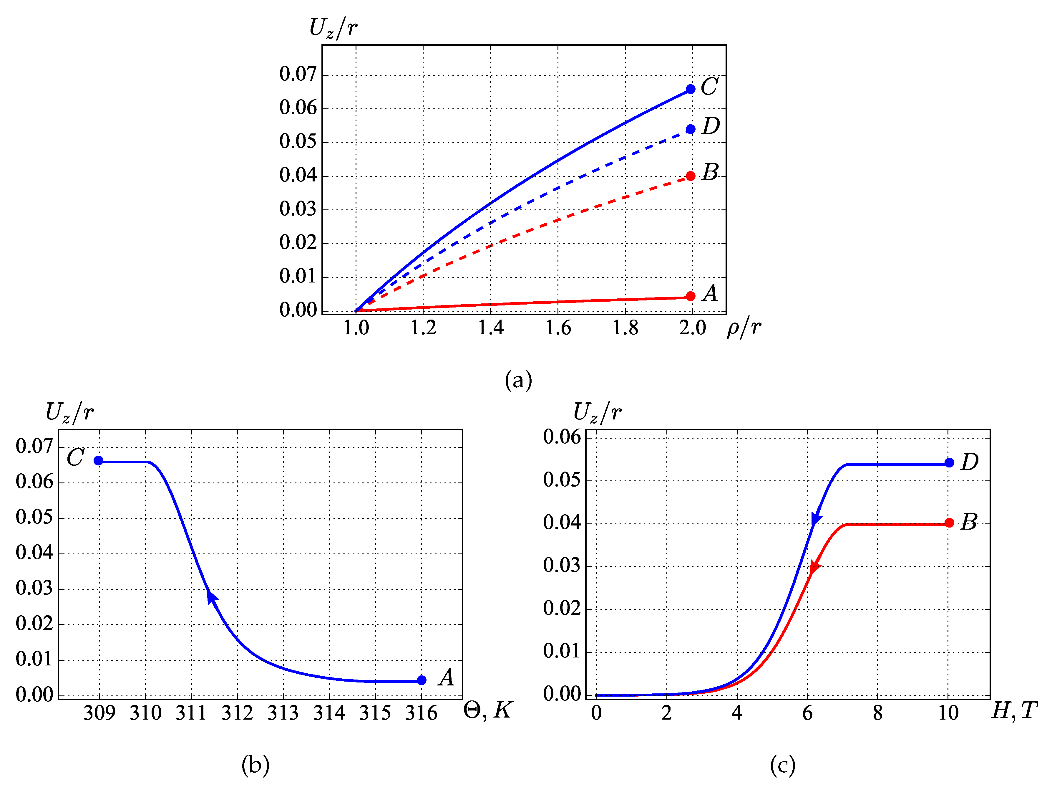
In Figure 4a, the red solid line represents the distribution of the axial displacement along the radius in the case when the shift of the outer surface occurs in the austenitic state at the specified displacement or under the action of the respective force (initially giving rise only to elastic strains), and the red dashed line shows the distribution of axial displacement after the direct phase transition at a fixed shift of the outer surface , followed by complete unloading of this surface in the martensitic state. Cooling of the sample is responsible for the development of phase strains, which can cause additional deformation of the sample in the absence of fixed displacements of the outer surface. Therefore, during unloading, the displacement of the external surface of the sample increases, realizing thus the accumulated strains. In the same figure, the blue solid line represents the distribution of the axial displacement after the direct phase transition under the action of a fixed force on the outer surface , , and the blue dotted line describes the distribution of the axial displacement after the direct phase transition under the action of a fixed force on the outer surface followed by complete unloading of this surface in the martensitic state. In this case, the phase strains immediately cause the macroscopic deformation of the sample, whereas during unloading, the displacement of the external surface of the sample decreases, due to the removal of elastic strains. Points correspond to the axial displacements of the outer surface and coincide with the points shown in Figure 3.
Figure 4b shows the dependence of the axial displacement of the outer surface on temperature (a direct phase transition during cooling under the action of a fixed force on the outer surface , ). The initial and finite values of the displacement are marked by letters A and C, which correspond to the same points in Figure 3 and Figure 4a. A decrease in the temperature causes, in addition to the elastic displacement, the axial displacement of the outer surface due to the resulting phase strains.
Figure 4c shows the dependence of the axial displacement of the outer surface on the magnetic field H. The initial values denoted by letters B and D correspond to the applied magnetic field of 10 T and the heating of the cylinder to a temperature higher than . They are almost similar to the displacements in the unloaded state denoted in Figure 3 and Figure 4a by the same letters, since the thermal strains and the strains caused by the applied magnetic field are small compared to already existing phase strains. When the magnetic field decreases to 0 T, the sample reverts to the original state (the path is indicated by arrows; the red line corresponds to the problem in which a direct austenite-martensite phase transition was carried out at a fixed displacement, and the blue line to the problem in which a direct austenite-martensite phase transition was carried out under the action of a fixed force), and the outer surface of the cylinder shifted by a prescribed displacement or force returns to its initial position. This figure demonstrates the possibility of a reverse phase transition at a constant temperature under sequential removal of the magnetic field applied in the martensitic state.
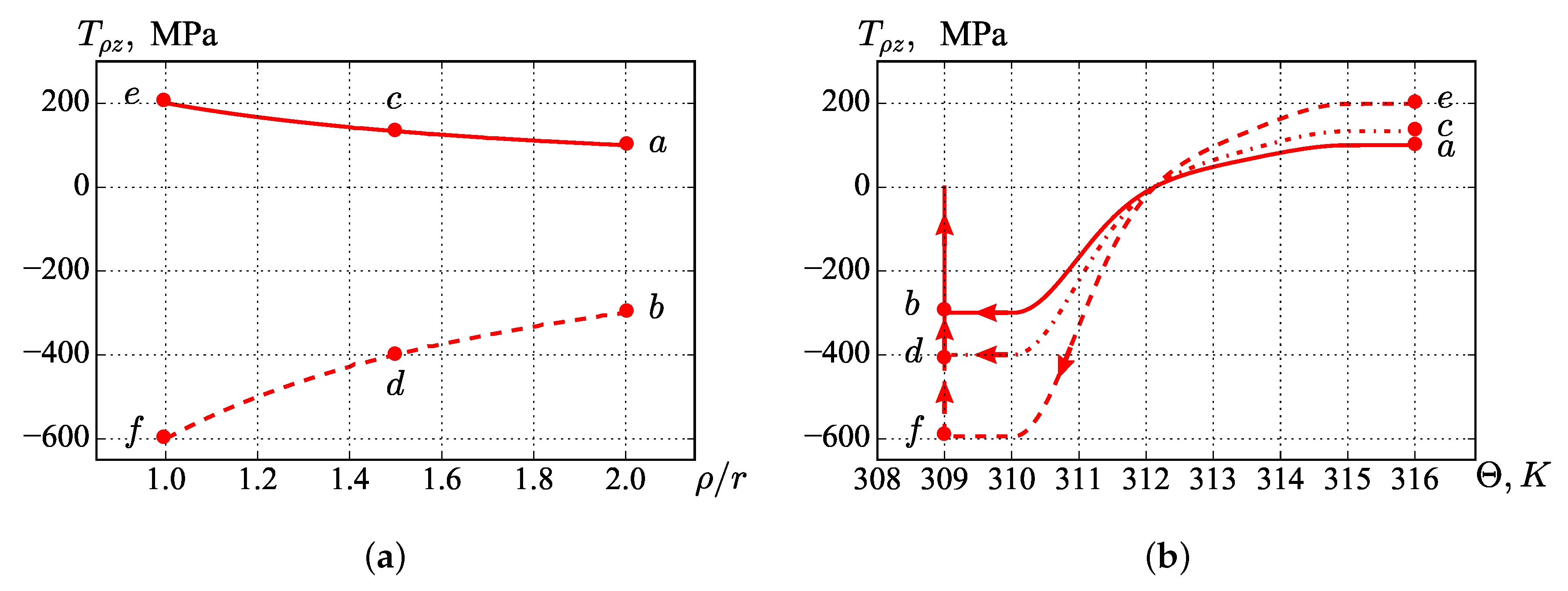
In Figure 5a, the solid line corresponds to the distribution of the axial component of the true stress tensor along the radius in the case when the shift of the outer surface occurs in the austenitic state (elastic solution), and the dotted line shows the stress distribution after the direct phase transition (in the martensitic state) at a fixed displacement of the outer surface. It is seen that after the direct phase transition, the stress is negative along the entire radius of the cylinder, since the resulting phase strains at a fixed displacement of the outer surface lead to negative elastic strains. Points correspond to the shear stresses on the outer surface, points in the midsection, and points on the inner surface.
Figure 5b shows the dependence of the axial force applied to the outer surface (solid line), to the midsection (dash-dotted line), and to the inner surface (dashed line) on temperature (direct phase transition during cooling at a fixed displacement of the outer surface and subsequent force removal). Points correspond to the same points in Figure 5a. With decreasing temperature, the shear forces decrease, and at a temperature of , the sample is completely unloaded; under subsequent cooling, the shear forces become negative. For the unloaded outer surface (, corresponding to points b, tends to zero) and the fixed inner surface, in the midsection and at the inner surface, corresponding to points d and f, also tend to zero.
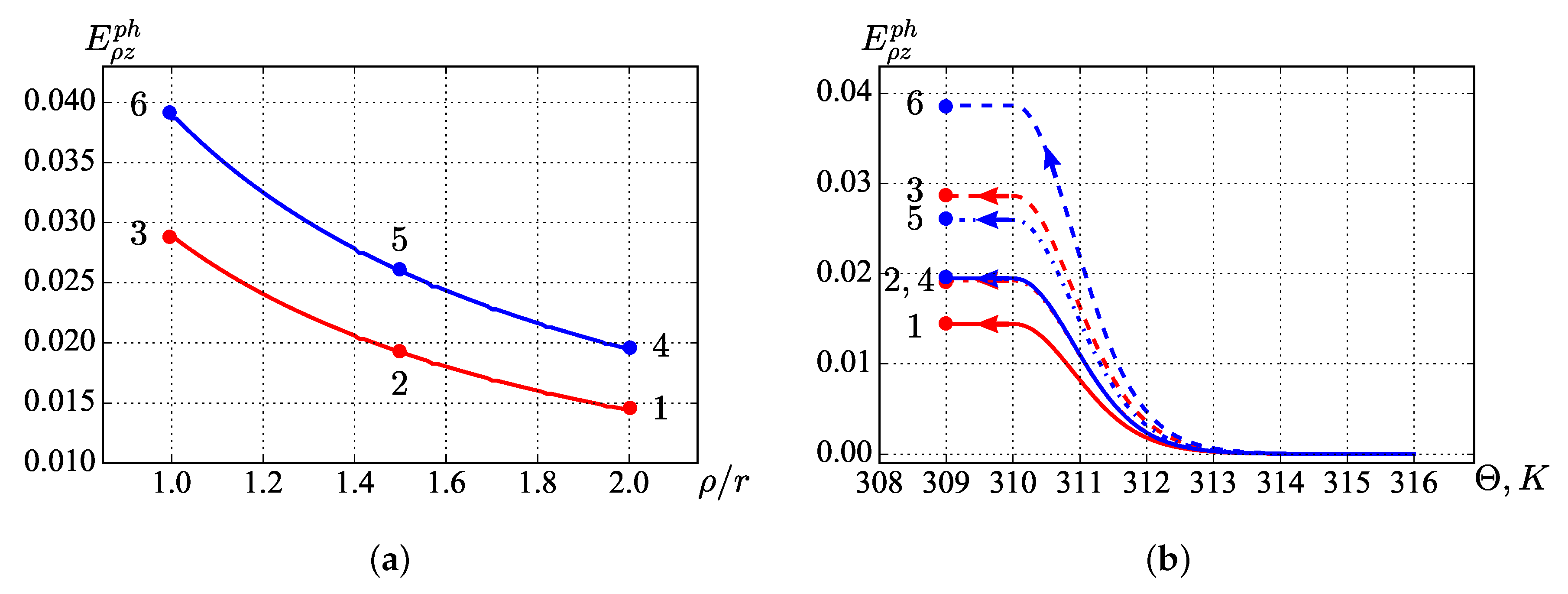
Figure 6a shows the distribution of the shear component of the phase strain tensor along the radius. The red line is the result of the solution obtained for the phase transition at a fixed displacement of the outer surface and the blue line under the action of a fixed force. It can be seen from the figure that cooling under the action of a fixed force leads to greater phase strains compared to cooling at a fixed displacement, since in the second case, the stresses decrease throughout the sample, which slows down the development of phase strains. Points correspond to the phase strains on the outer surface of the cylinder; Points in the midsection, and Points on the inner surface.
6. Conclusions
The boundary value problem of the accumulation and recovery of phase strains in a long hollow cylinder made of a ferromagnetic shape memory alloy was solved in the framework of the model, describing the behavior of shape memory alloys under finite deformations. It was shown that during the direct phase transition, the magnitudes of accumulated phase strains depend on the boundary conditions. Complete removal of the accumulated strains in the sample occurred on heating to the temperatures characteristic of the reverse phase transition and also at a constant temperature when the magnetic field previously applied in the martensitic state was removed. The latter observation was confirmed by the fact that the outer surface of the ferromagnetic cylinder, experiencing an axial shift in the austenitic state (growing essentially during martensitic transformation) returns to its initial position.
It should be noted that the effect of returning the external cylinder surface previously shifted in the axial direction to the original position was considered in [29,30]. However, in these studies, the resetting of the outer surface is associated with changes in the quantities, which, in the problems describing the behavior of a slightly compressed isotropic elastic material during finite deformations, are interpreted as shear moduli and bulk moduli and increase due to the application of high hydrostatic pressure or under strongly-constrained deformation.
Author Contributions
The authors contributed equally to this work.
Funding
The reported study was funded by RFBR and Perm Krai according to the research project 19-41-590008.
Acknowledgments
The authors are very much obliged to L. V. Semukhina for her assistance in preparation of the English version of the paper.
Conflicts of Interest
The authors declare no conflict of interest.
References
- Lagoudas, D.C. Modeling and Engineering Applications; Springer Science+Business Media: New York, NY, USA, 2008; p. 455. [Google Scholar]
- Haldar, K.; Lagoudas, D.C.; Karaman, I. Magnetic field-induced martensitic phase transformation in magnetic shape memory alloys: Modeling and experiments. J. Mech. Phys. Solids 2014, 69, 33–66. [Google Scholar] [CrossRef]
- Chen, X.; Moumni, Z.; He, Y.; Zhang, W. A three-dimantional model of magneto-mechanical behaviors of martensite reorientation in ferromagnetic shape memory alloys. J. Mech. Phys. Solids 2014, 64, 249–286. [Google Scholar] [CrossRef]
- Roubíček, T.; Stefanelli, U. Magnetic shape-memory alloys: Thermomechanical modelling and analysis. Continuum Mech. Thermodyn. 2014, 26, 783–810. [Google Scholar] [CrossRef]
- Khan, R.A.A.; Ghomashchi, R.; Xie, Z.; Chen, L. Ferromagnetic shape memory Heusler materials: Synthesis, microstructure characterization and magnetostructural properties. Materials 2018, 11, 988. [Google Scholar] [CrossRef] [PubMed]
- Sakon, T.; Fujimoto, N.; Kanomata, T.; Adachi, Y. Magnetostriction of Ni2Mn1−xCrxGa Heusler Alloys. Metals 2017, 7, 410. [Google Scholar] [CrossRef]
- Sakon, T.; Adachi, Y.; Kanomata, T. Magneto-structural properties of Ni2MnGa ferromagnetic shape memory alloy in magnetic fields. Metals 2013, 3, 202–224. [Google Scholar] [CrossRef]
- Buchel’nikov, V.D.; Vasil’ev, A.N.; Koledov, V.V.; Taskaev, S.V.; Khovailo, V.V.; Shavrov, V.G. Magnetic shape-memory alloys: Phase transitions and functional properties. Phys. Uspekhi Adv. Phys. Sci. 2006, 49, 871–877. [Google Scholar] [CrossRef]
- Cherechukin, A.A.; Dikstein, I.E.; Ermakov, I.E.; Glebov, A.V.; Koledov, V.V.; Kosolapov, D.A.; Shavrov, V.G.; Tulaikova, A.A.; Krasnoperov, E.P.; Takagi, T. Shape memory effect due to magnetic field induced thermoelastic martensitic transformation in polycrystalline Ni–Mn–Fe–Ga alloy. Phys. Lett. A 2001, 291, 175–183. [Google Scholar] [CrossRef]
- Cherechukin, A.A.; Khovailo, V.V.; Koposov, R.V.; Krasnoperov, E.P.; Takagi, T.; Tani, J. Training of the Ni–Mn–Fe–Ga ferromagnetic shape-memory alloys due cycling in high magnetic field. J. Magn. Magn. Mater. 2003, 258, 523–525. [Google Scholar] [CrossRef]
- Malygin, G.A. Theory of magnetic shape memory effect and pseudoelastic deformation in Ni–Mn–Ga alloys. Phys. Solid State 2009, 51, 1694–1699. [Google Scholar] [CrossRef]
- Bustamante, R.; Dorfman, A.; Ogden, R.W. Universal relations in isotropic nonlinear magnetoelasticity. Q. J. Mech. Appl. Math. 2006, 59, 435–450. [Google Scholar] [CrossRef] [Green Version]
- Bustamante, R.; Dorfman, A.; Ogden, R.W. A nonlinear magnetoelastic tube extansion and inflation in an axial magnetic field: Numerical solution. J. Eng. Math. 2007, 59, 139–153. [Google Scholar] [CrossRef]
- Bustamante, R.; Dorfman, A.; Ogden, R.W. Numerical solution of finite geometry boundary-value problems in nonlinear magnetoelasticity. Int. J. Solids Struct. 2011, 48, 874–883. [Google Scholar] [CrossRef] [Green Version]
- Luré, A.I. Nonlinear Elasticity Theory; Nauka: Moscow, Russia, 1980; p. 512. (In Russian) [Google Scholar]
- Truesdell, C. A First Course in Rational Continuum Mechanics; John Hopkins University: Baltimore, MD, USA, 1972. [Google Scholar]
- Rogovoy, A.A. Formalized approach to construction of the state equations for complex media under finite deformations. Continuum Mech. Thermodyn. 2012, 24, 81–114. [Google Scholar] [CrossRef]
- Rogovoy, A.A. Differentiation of scalar and tensor functions of tensor argument. IOSR J. Math. 2019, 15, 1–20. [Google Scholar]
- Liu, Y.; Gall, K.; Dunn, M.L.; Greenberg, A.R.; Diani, J. Thermomechanics of shape memory polymers: Uniaxial experiments and constitutive modeling. Int. J. Plast. 2006, 22, 279–313. [Google Scholar] [CrossRef]
- Baghani, M.; Naghdabadi, R.; Arghavani, J.; Sohrabpour, S. A thermodynamically-consistent 3D constitutive model for shape memory polymers. Int. J. Plast. 2012, 35, 13–30. [Google Scholar] [CrossRef]
- Baghani, M.; Naghdabadi, R.; Arghavani, J. A large deformation framework for shape memory polymers: Constitutive modeling and finite element implementation. J. Intell. Material Syst. Struct. 2013, 24, 21–32. [Google Scholar] [CrossRef]
- Rogovoi, A.; Stolbova, O. Modeling the magnetic field control of phase transition in ferromagnetic shape memory alloys. Int. J. Plast. 2016, 85, 130–155. [Google Scholar] [CrossRef]
- Movchan, A.A.; Chzho, T.I. Solution of boundary problems of forward and inverse transformations in the framework of nonlinear deformation theory of shape memory alloys. Mech. Comput. Mater. Struct. 2007, 13, 452–468. (In Russian) [Google Scholar]
- Movchan, A.A.; Shelymagin, P.V.; Kazarina, S.A. Constitutive equations for two-step thermoelastic phase transformations. J. Appl. Mech. Tech. Phys. 2001, 42, 864–871. [Google Scholar] [CrossRef]
- Bozorth, R.M. Ferromagnetism; Wiley: New York, NY, USA, 1993. [Google Scholar]
- Raikher, Y.L.; Stolbov, O.V.; Stepanov, G.V. Deformation of a circular ferroelastic membrane in a uniforn magnetic field. Tech. Phys. 2008, 53, 1169–1176. [Google Scholar] [CrossRef]
- Luré, A.I. Elasticity Theory; Nauka: Moscow, Russia, 1970; p. 940. (In Russian) [Google Scholar]
- Kachanov, M.; Shafiro, B.; Tsukrov, I. Handbook of Elasticity Solutions; Springer Science+Business Media: Dordrecht, The Netherlands, 2003; p. 324. [Google Scholar]
- Kuznetsova, V.G.; Rogovoy, A.A. The effect of taking into account the slight compressibility of the material in elastic problems with finite deformations. Izvestiya RAN. MTT 2000, 6, 25–37. (In Russian) [Google Scholar]
- Rogovoy, A. Effect of elastomer slight compressibility. Eur. J. Mech. A Solids. 2001, 20, 757–775. [Google Scholar] [CrossRef]
Figure 1.
Phase transition diagram.

Figure 2.
Sample.

Figure 3.
Displacement history of the points of the cylinder section.

Figure 4.
Displacements in the sample: distribution along the radius (a) and dependence on temperature (b) and on the magnetic field (c).
Figure 4.
Displacements in the sample: distribution along the radius (a) and dependence on temperature (b) and on the magnetic field (c).

Figure 5.
Shear force: distribution along the radius (a) and temperature dependence (b).

Figure 6.
Phase strains: distribution along the radius (a) and dependence on temperature (b).

© 2019 by the authors. Licensee MDPI, Basel, Switzerland. This article is an open access article distributed under the terms and conditions of the Creative Commons Attribution (CC BY) license (http://creativecommons.org/licenses/by/4.0/).
Share and Cite
MDPI and ACS Style
Rogovoy, A.A.; Stolbova, O.S. Numerical Simulation of the Phase Transition Control in a Cylindrical Sample Made of Ferromagnetic Shape Memory Alloy. Computation 2019, 7, 38. https://0-doi-org.brum.beds.ac.uk/10.3390/computation7030038
AMA Style
Rogovoy AA, Stolbova OS. Numerical Simulation of the Phase Transition Control in a Cylindrical Sample Made of Ferromagnetic Shape Memory Alloy. Computation. 2019; 7(3):38. https://0-doi-org.brum.beds.ac.uk/10.3390/computation7030038
Chicago/Turabian StyleRogovoy, Anatoli A., and Olga S. Stolbova. 2019. "Numerical Simulation of the Phase Transition Control in a Cylindrical Sample Made of Ferromagnetic Shape Memory Alloy" Computation 7, no. 3: 38. https://0-doi-org.brum.beds.ac.uk/10.3390/computation7030038
Note that from the first issue of 2016, this journal uses article numbers instead of page numbers. See further details here.