Design and Implementation of a Microcontroller Based Active Controller for the Synchronization of the Petrzela Chaotic System

Abstract

This paper presents an active control design for the synchronization of two identical Petrzela chaotic systems (Petrzela, J.; Gotthans, T. New chaotic dynamical system with a conic-shaped equilibrium located on the plane structure. Applied Sciences. 2017, 7, 976) on master-slave configuration. For the active control, the parameters of both systems are assumed to be a priori known, the control law by means of the dynamic of the error synchronization is designed to guarantee the convergence to zero of error states and the synchronization process is verified by numerical simulation. By taking advantage of the execution and implementation facilities of microcontroller based chaotic systems in digital devices, the active controller is implemented in a 32 bits ARM microcontroller. The experimental results were obtained by using the fourth order Runge-Kutta numerical method to integrate the differential equations of the controller, where the results were measured with a digital oscilloscope.

1. Introduction

In recent decades, chaotic systems have been studied due to their nonlinear dynamic properties and for the possible applications they have in different fields of science. This began due to the work of references [1,2] in which they showed that synchronization of chaotic systems is possible; this development has been utilized in areas such as secure communications [3,4,5], cryptography [6,7], medical applications, mechanisms, and robotics [8,9,10,11,12,13,14,15]. Some of the synchronization schemes that have been successfully developed and applied include linear and nonlinear feedback control [16,17,18,19,20,21,22,23,24,25], where a Lyapunov candidate function V is proposed in such a way that the control law selected from the first derivative of V must be defined as negative [25]. Adaptable control [16,17,18,19,26,27] is of interest for the synchronization of chaotic systems because of the presence of unknown parameters since the learning laws are continuously updated for maintaining the performance of the system. Other controls are also applied, for example the control by state feedback [28,29,30,31,32,33,34], feedback control with delays [35,36,37,38] or active control [39,40,41,42] which works by considering the error synchronization, here the nonlinearities are eliminated, and the dynamic error equations are decoupled. Finally, synchronization has been used through neural networks [43].

It is often thought that chaotic systems have a combination of several chair-type equilibrium points that produce the evolution of the chaotic attractor. However, systems with infinite points of equilibrium can be observed, located along a line [44,45], surface [46], or in closed curves [47] which fall into a new category of chaotic systems with a hidden attractor. In general, to be able to use chaotic systems in engineering applications, it is necessary to have a real implementation of them by means of analog electronic devices [48,49] or embedded systems [50]. The implementation of chaotic systems in embedded devices such as microcontrollers [50,51,52,53], digital signal processors (DSP), or field programmable gate array (FPGA) [4,54,55,56], have advantages in comparison with the implementation of circuits with analog components such as operational amplifiers and multipliers. Some of the advantages include a higher velocity of implementation, high computational power, low power consumption and precision because the resistors and capacitors have tolerance problems, which do not greatly change their value with respect to temperature [50]. In addition, working with digital devices allows us to specify delays in the implementation, opening the possibility of investigating differential equations with chaotic delays [55,57]. Authors in reference [52] perform the synchronization of Genesio & Tesi multi-scroll chaotic systems by neural network identifier into a microcontroller Arduino UNO^®. One advantage of this method is that the plant model to be synchronized and its parameters are unknown. Although a small error value persists, the synchronization holds the error signals bounded in a very small region.

In robotic, the chaotic systems applications are focused on mobile robotic and collaborative systems. For mobile robotics applications, robots are used for exploration and search for civil and military applications. The tasks they perform are target identifications, robot positioning on the ground, or updating maps. In the monitoring of security systems, chaotic paths are induced to the mobile in such a way that knowing its future position become unpredictable. In search and rescue applications (natural disasters), the robot must navigate in highly irregular and erratic environments, using chaotic motion planning techniques to ensure a quick search in the entire workspace. Therefore, the possibility of proposing navigation paths based on chaotic systems and their implementation in analog and embedded electronic systems remains open [12,13,14].

Considering the above, this article presents the design and implementation of an active controller in a 32-bit microcontroller for the synchronization in a master-slave configuration of the Petrzela chaotic system. To the best knowledge of the authors, this type of synchronization and neither this type of control has been used for this new system. Then, the article is organized as follows: Section 2 describes the characteristics of the chaotic system, Section 3 explains the active control and demonstrates by means of numerical simulations the successful synchronization of the dynamic system. In Section 4 the results of the microcontroller implementation are discussed and the conclusions of the paper are provided.

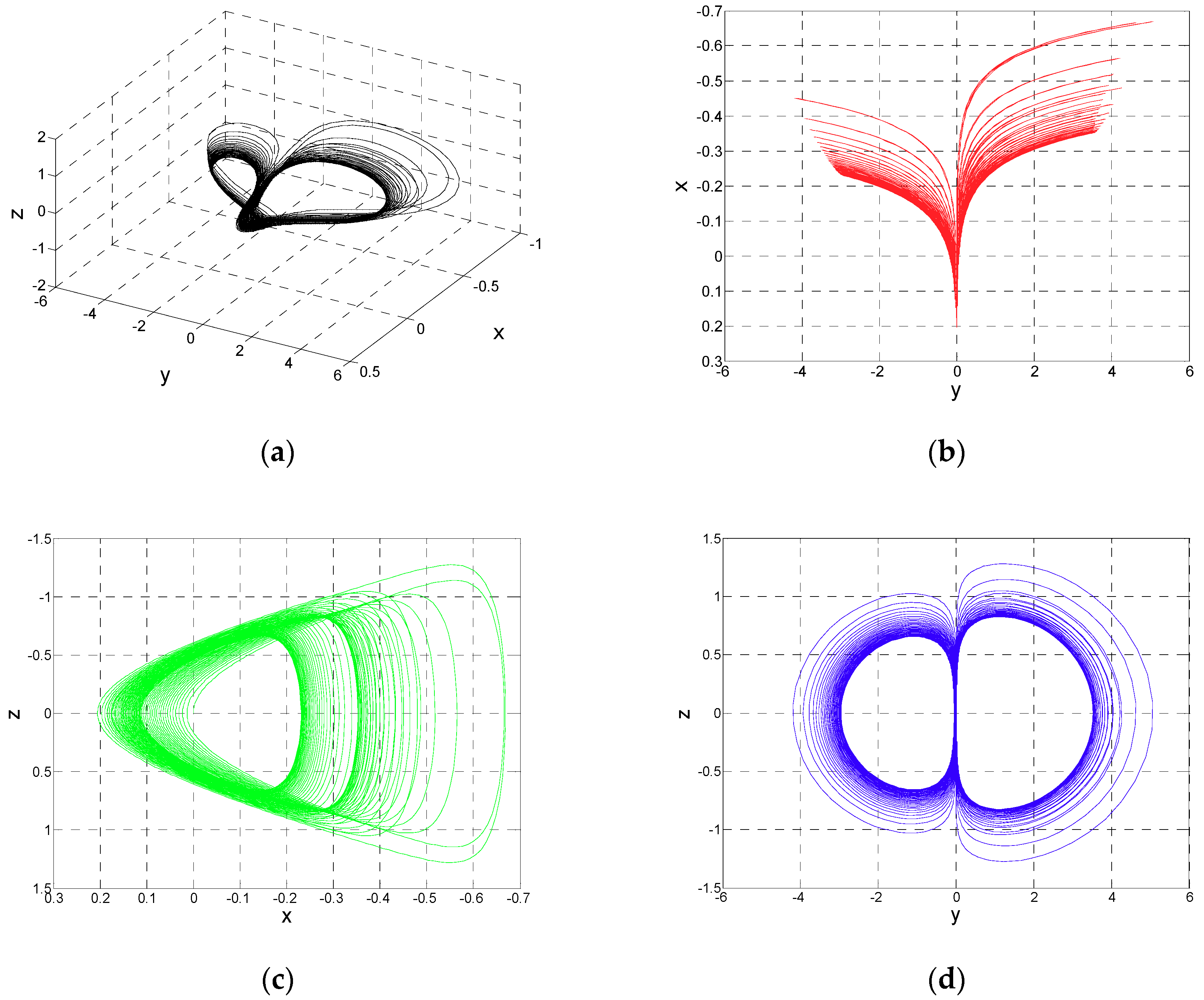
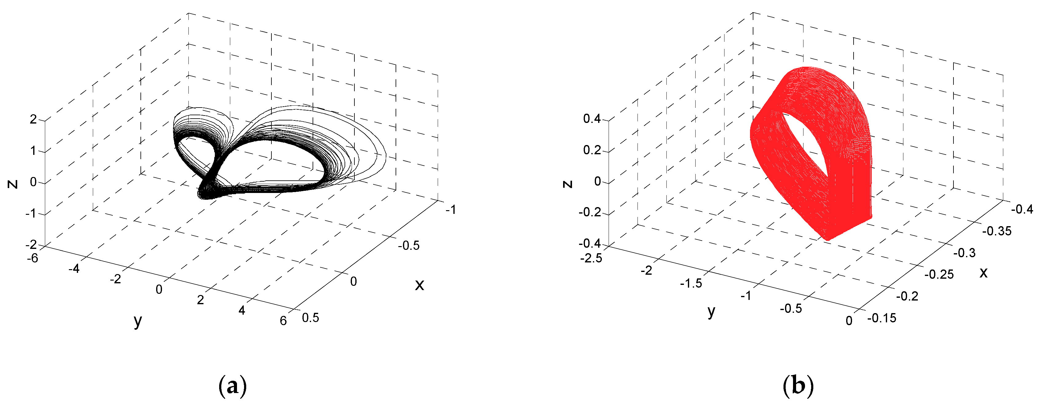
2. Petrzela Chaotic System

The chaotic system is presented with the following differential equations:

$$\begin{array}{c}\dot{x}=z\\ \dot{y}=-ayz-bx{z}^2\\ \dot{z}=x+y^2-r\end{array}$$

(1)

where a and b are the internal parameters of the system, they are used to observe different routes and the evolution of the strange attractor, while $r$ represents the displacement of the hyperbolic equilibrium structure, it could be a fixed value.

Through the Jacobian matrix (2), it is possible to find the characteristic Equation (3) as a function of points on a hyperbolic equilibrium structure;

$$J\left(x\right)=\left(\begin{array}{ccc}0& 0& 1\\ -b{z}^2& -az& -ay-2bxz\\ 1& 2y& 0\end{array}\right),$$

(2)

$$\begin{gathered} \left|\left(\lambda I-J\left(x\right)\right)\right|=\left|\left(\begin{array}{ccc}\lambda & 0& -1\\ b{z}^2& \lambda +az& ay+2bxz\\ -1& -2y& \lambda \end{array}\right)\right|, \\ ={\lambda }^3+az{\lambda }^2+\left(2a{y}^2+4bxyz-1\right)\lambda +2by{z}^2-az=0, \end{gathered}$$

(3)

Considering the equilibrium plane $z=0$ and by using the parameterization curve, the following simplified characteristic equation with its eigenvalues is obtained:

$$\begin{gathered} ={\lambda }^3+\left(2a{y}^2-1\right)\lambda =\lambda \left({\lambda }^2+2a{y}^2-1\right)=0, \\ \Rightarrow \hspace{1em}{\lambda }_1=0;{\lambda }_{2,3}=\pm \sqrt{1-2a{y}^2}, \end{gathered}$$

(4)

In this case ${\lambda }_1$ is always zero, ${\lambda }_{2,3}$ are real with opposite signs when $y<1/\sqrt{2a}$; it is a complex conjugate imaginary pair if $y>1/\sqrt{2a}$, and equal to zero if $y=1/\sqrt{2a}$. Depending on the initial conditions near the equilibrium, the system can be leads to periodic oscillations. In this case, there is a coexistence of three types of solutions which are: limit cycles, chaos and unbounded. In addition, the dynamic movement is invariant under changes of coordinates $y\leftrightarrow -y$ and $z\leftrightarrow -z$.

Numerical Analysis of the Chaotic System

Two of the most used methods to resolve differential equations of chaotic systems are Euler 1st order and Runge-Kutta 4th order numerical algorithms [4,50,51,52,53,54,55,56]. Euler is a straight-forward method, quick and it is easy to code, although its accuracy is poor. The Runge-Kutta method is not as fast but offers good computational performance and more accurate solutions than Euler method, because the truncation error is reduced in higher orders methods. With the fourth order numerical Runge-Kutta integration method the solution of the system (1) can be found, for an initial condition in which it was considered; $x_0={\left(000\right)}^T$, a simulation time $t_{max}=150$ s, a time step of ${\Delta }_t=0.01$, and constant values of $a=12, b=0.4$ and $r=1$, the behavior of the Petrzela system is shown in Figure 1.

3. Synchronization with Active Control

In this section, the active control is applied to synchronize two identical chaotic systems type (1) with different initial conditions between them. The aim of the synchronization is that the slave system follows the dynamic behavior of the master system, which is achieved by applying an appropriate control law $u={\left[u_1 u_2 u_3\right]}^T$ to the slave system; therefore, the master system is given as follows:

$$\begin{array}{c}{\dot{x}}_m=z_m\\ {\dot{y}}_m=-a{y}_m{z}_m-b{x}_m{z}_m^2\\ {\dot{z}}_m=x_m+y_m^2-r\end{array},$$

(5)

The master slave is given by:

$$\begin{array}{c}{\dot{x}}_s=z_s+u_1\\ {\dot{y}}_s=-a{y}_s{z}_s-b{x}_s{z}_s^2+u_2\\ {\dot{z}}_s=x_s+y_s^2-r+u_3\end{array},$$

(6)

The synchronization process is performed by calculating the synchronization error $e={\left[e_1 e_2 e_3\right]}^T$, which is defined as the difference between the state of the master system (5) and the state of the slave system (6), represented by:

$$\begin{array}{c}{e}_1=x_s-x_m\\ e_2=y_s-y_m\\ e_3=z_s-z_m\end{array},$$

(7)

By applying the derivative to the synchronization errors in (7) and substituting the Equations (5) and (6), the dynamics of the synchronization error is obtained by:

$$\begin{array}{c}{\dot{e}}_1={\dot{x}}_s-{\dot{x}}_m=z_s+u_1-z_m\\ {\dot{e}}_2={\dot{y}}_s-{\dot{y}}_m=-a{y}_s{z}_s-b{x}_s{z}_s^2+u_2+a{y}_m{z}_m+b{x}_m{z}_m^2\\ {\dot{e}}_3={\dot{z}}_s-{\dot{z}}_m=x_s+y_s^2-r+u_3-x_m-y_m^2+r\end{array}$$

(8)

Rearranging the terms to be expressed as a function of the errors, taken from (7), and substituting $y_s{z}_s=\left(e_2+y_m\right)\left(e_3+z_m\right); x_s{z}_s^2=(e_1+x_m){\left(e_3+z_m\right)}^2$, Equation (8) is simplified to obtain the following:

$$\begin{array}{c}{\dot{e}}_1=e_3+u_1\\ {\dot{e}}_2=-b{e}_3^2{x}_m-a{e}_3{y}_m-a{e}_2{z}_m-2b{e}_1{e}_3{z}_m-2b{e}_3{x}_m{z}_m-b{e}_1{z}_m^2-a{e}_2{e}_3-b{e}_1{e}_3^2+u_2,\\ {\dot{e}}_3=2e_2{y}_m+e_1+e_2^2+u_3\end{array}$$

(9)

From this Equation (9), in order to eliminate the nonlinearities and to uncouple the equations of the dynamics error, the control laws are deduced as follows:

$$\begin{array}{c}{u}_1=-e_3-k_1{e}_1\\ u_2=b{e}_3^2{x}_m+a{e}_3{y}_m+a{e}_2{z}_m+2b{e}_1{e}_3{z}_m+2b{e}_3{x}_m{z}_m+b{e}_1{z}_m^2+a{e}_2{e}_3+b{e}_1{e}_3^2-k_2{e}_2,\\ u_3=-2e_2{y}_m-e_1-e_2^2-k_3{e}_3\end{array}$$

(10)

Substituting the control laws (10) in (9), the synchronization error dynamic is simplified as shown in (11):

$$\begin{array}{c}{\dot{e}}_1=-k_1{e}_1\\ {\dot{e}}_2=-k_2{e}_2\\ {\dot{e}}_3=-k_3{e}_3\end{array}=\left[\begin{array}{ccc}-k_1& 0& 0\\ 0& -k_2& 0\\ 0& 0& -k_3\end{array}\right]\left[\begin{array}{c}{e}_1\\ e_2\\ e_3\end{array}\right]=Ke,$$

(11)

A linear system is obtained as a function of the state errors $e={\left[e_1 e_2 e_3\right]}^T$. There are many possible options for the selection of the gains $k_1,k_2$ and $k_3$ that allows us to control the speed of convergence and to make stabilization of the system possible (11). By using the characteristic matrix of the closed loop system, the gains can be selected in such a way that all the eigenvalues are negative real parts as shown in (12).

$$\begin{gathered} \det \left|\lambda I-K\right|=\left[\begin{array}{ccc}\lambda +k_1& 0& 0\\ 0& \lambda +k_2& 0\\ 0& 0& \lambda +k_3\end{array}\right], \\ =\left(\lambda +k_1\right)\left(\lambda +k_2\right)\left(\lambda +k_3\right)\hspace{1em}\Rightarrow \hspace{1em}{\lambda }_1=-k_1; {\lambda }_2=-k_2; {\lambda }_3=-k_3, \end{gathered}$$

(12)

In this way, the state errors converge to zero $e\to 0$, while the time tends to infinity $t\to \infty$, implying that the chaotic systems (5) and (6) reach synchronization with the active control.

Stability Proof

The stability of the error dynamic (11) is determined by Lyapunov analysis. To achieve this, a positive defined function is proposed:

$$V:=\frac{1}{2}{e}_1^2+\frac{1}{2}{e}_2^2+\frac{1}{2}{e}_3^2,$$

(13)

The first derivative is given by

$$\dot{V}:=e_1\dot{e_1}+e_2\dot{e_2}+e_3\dot{e_3},$$

(14)

Substituting (11) in (14) and making algebraic operations,

$$\dot{V}:=-k_1{e}_1^2-k_2{e}_2^2-k_3{e}_3^2,$$

(15)

The objective is that $\dot{V}$ be negative defined $\dot{V}<0$ to guarantee the asymptotic convergence to zero of the error synchronization. It can be seen in (15) that if $k_1>0,k_2>0$ and $k_3>0$ then $\dot{V}<0$ the objective will be achieved according with the stability theorem of Lyapunov. By another hand, if $k_1\ge \frac{1}{2},k_2\ge \frac{1}{2}$ and $k_3\ge \frac{1}{2}$ then the following inequality is correct

$$-k_1{e}_1^2-k_2{e}_2^2-k_3{e}_3^2\le -\frac{1}{2}{e}_1^2-\frac{1}{2}{e}_2^2-\frac{1}{2}{e}_3^2,$$

(16)

In the right hand of the inequality (16), the same candidate Lyapunov function can be seen, but this version is negative.

$$\dot{V}\le -V,$$

(17)

That shows than $\dot{V}$ is bounded by the negative function of $V$. Solving the inequality (17) and making some algebraic operations, the Equation (18) is obtained:

$$\begin{gathered} \frac{d}{dt}V\le -V, \\ {{\displaystyle \int }}_{V\left(0\right)}^V\frac{d\left(V\right)}{-V}\le -{{\displaystyle \int }}_0^{t}d\tau , \\ \ln V-\ln V\left(0\right)\le -t, \\ V\le V\left(0\right)ex{p}^{-t}, \end{gathered}$$

(18)

Therefore

$$e_1^2+e_2^2+e_3^2\le \left(e_1^2\left(0\right)+e_2^2\left(0\right)+e_3^2\left(0\right)\right)e^{-t},$$

(19)

By applying square root to both members of (19)

$$e\le e\left(0\right)ex{p}^{-\frac{1}{2}t},$$

(20)

where $\Vert e\Vert$ is the Euclidean norm of $e={\left[e_1 e_2 e_3\right]}^T$. In this way, the exponential converge of error synchronization is guaranteed.

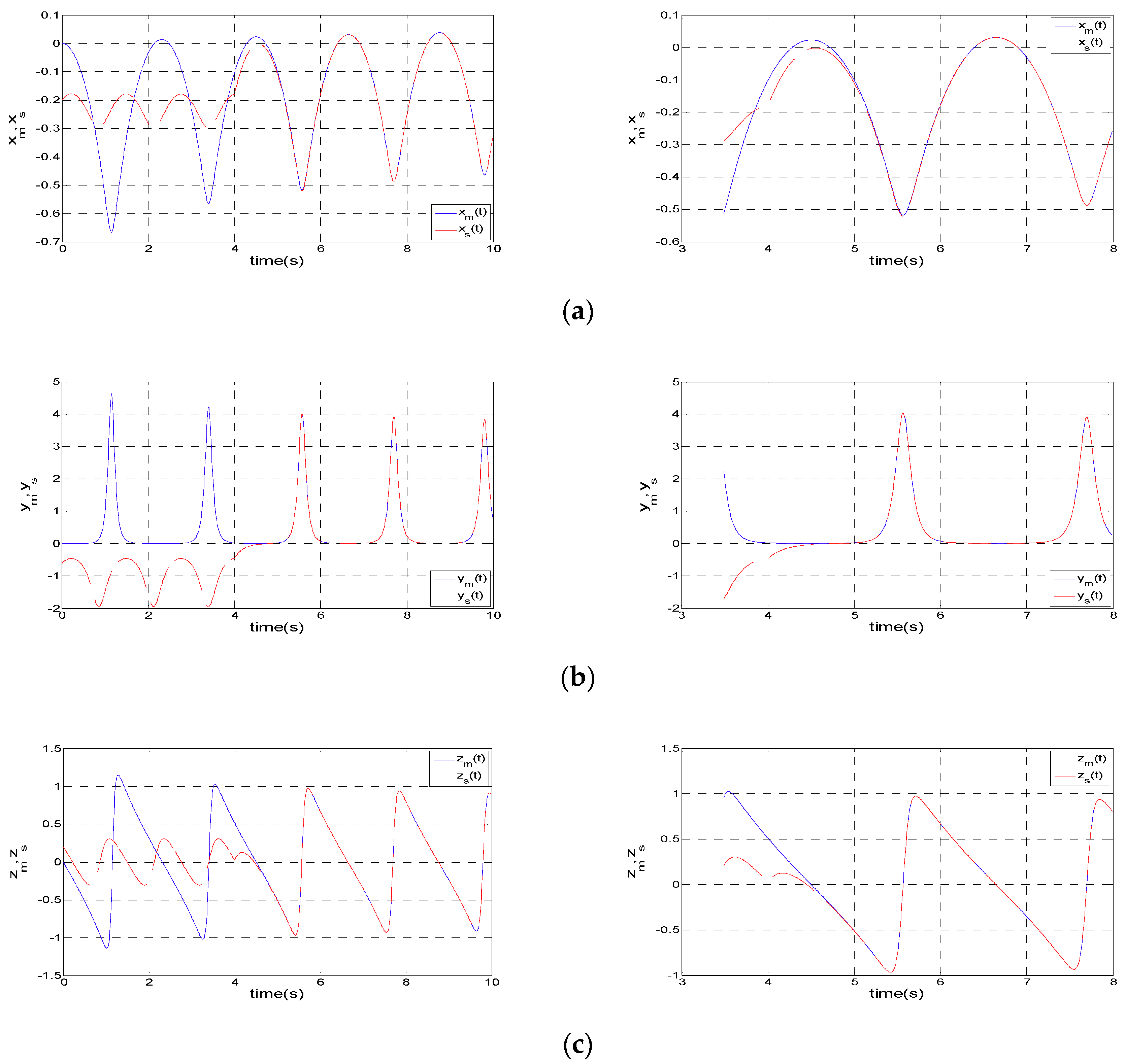
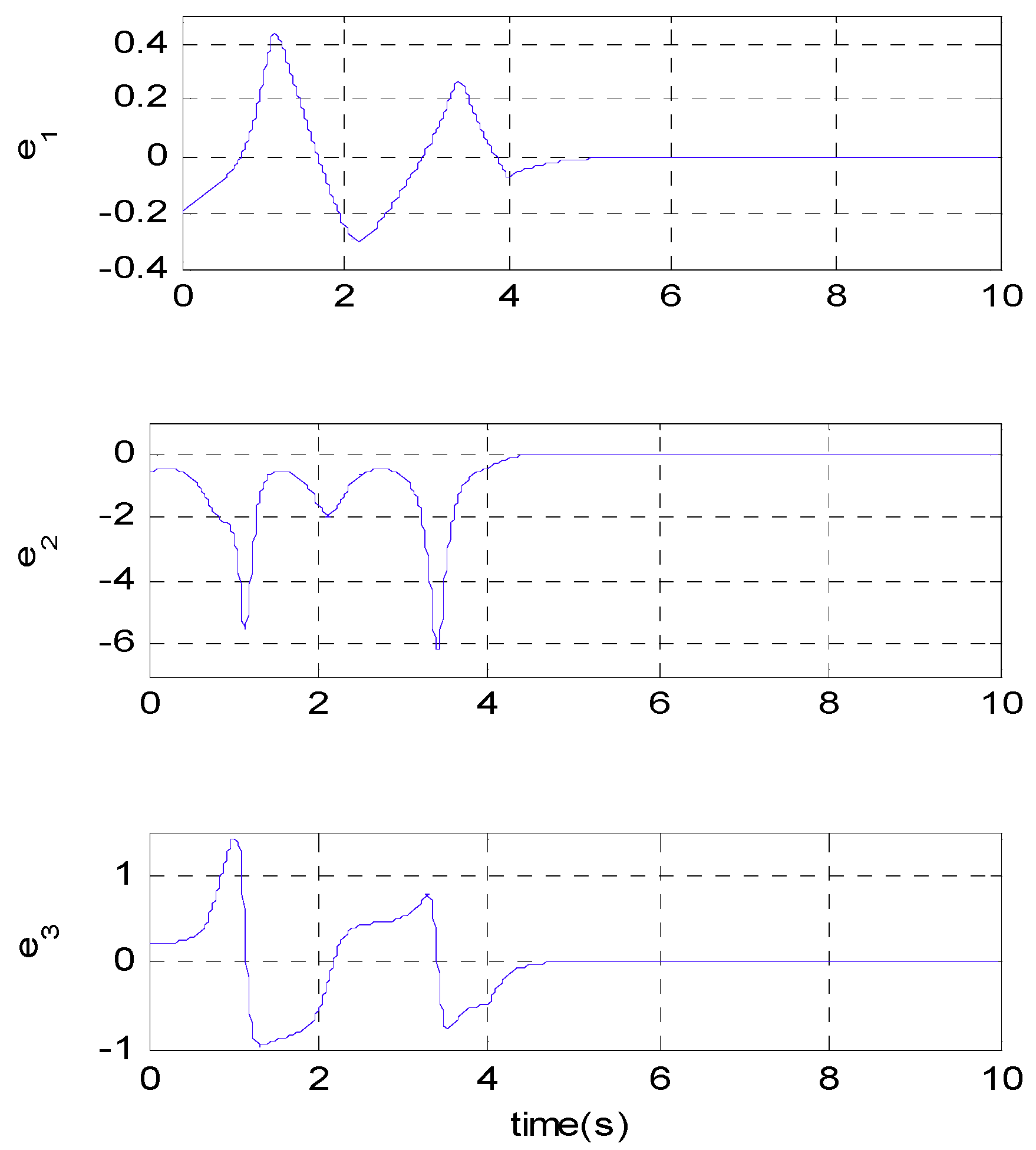
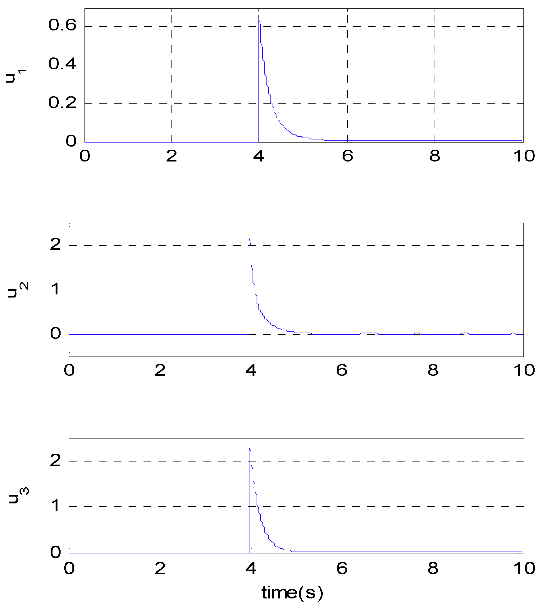
4. Numerical Results

This section presents the numerical simulation of the master-slave configuration for the systems (5) and (6). Figure 2a shows the attractor of the master system with initial condition $x_{m_0}={\left(0 0 0\right)}^T$, while the attractor of the slave system is shown in Figure 2b, which considers $x_{s_0}={\left(-0.2-0.6 0.2\right)}^T$. Both work during a simulation time of $t_{max}=150$s, with a time step of ${\Delta }_t=0.01$, as well as constants of $a=12, b=0.4$ and $r=1$.

Using the control laws of (10) and solving the system (11) of the synchronization error dynamics for $k_1=2,k_2=5 \mathrm{and} k_3=5$, Figure 3 shows the synchronization process between the states of the master and slave systems. During the first seconds t ≤ 4 s, it is observed how the evolution of each state is different, after four seconds t > 4 s the control laws are activated, then the states of slave system begins to follow the states of the master system, achieving synchronization in approximately 2 s (t = 6 s).

The right side of Figure 3a–c is like a zoomed-in version to more clearly visualize when the synchronization process begins.

In Figure 4, while t ≤ 4 s the synchronization errors have chaotic behavior, when t > 4 s the control laws begin to work, and the errors converge to zero.

In Figure 5 the input controls are shown, the value of $u={\left[u_1 u_2 u_3\right]}^T=0$ for t ≤ 4 s. Once t > 4 s the input control tends to zero.

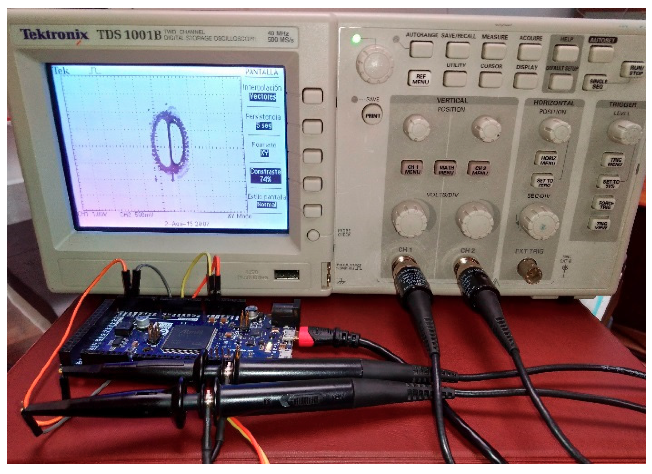
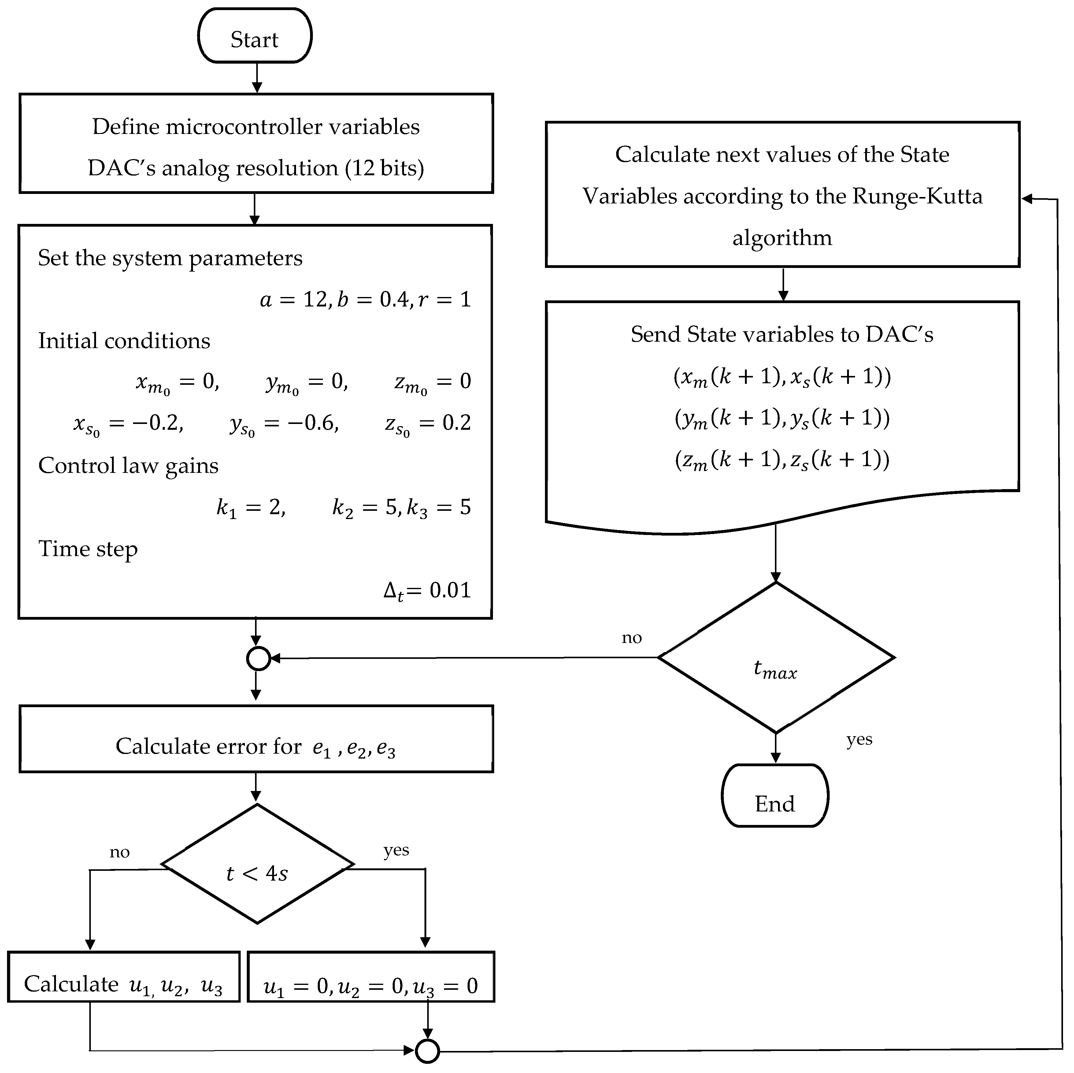
5. Hardware Implementation

The active controller was implemented in the Arduino DUE^® board, based on the Atmel SAM3X8E ARM^® Cortex^®-M3 CPU (manufactured by Arduino, made in Italy), because is open source. That has a processing speed up to 84 MHz. The main feature to choose the microcontroller was the two digital to analog converter peripherals DAC0 and DAC1 with 12 bits of resolution, in addition to its attractive cost benefit outcomes compared to FPGA or DSP devices. The hardware used for the active controller implementation is shown in Figure 6. For the synchronization process of the Petrzela systems, the synchronization error and the control law are calculated; later, the master and slave differential equations are solved by the Runge-Kutta method and are sent from the DAC’s to the oscilloscope.

To perform the implementation of the chaotic systems (5) and (6), the differential equations must be discretized, as is shown in Equation (21). The code is programmed inside the ARM microcontroller with its own language, which is based in processing programming language that is similar to C++. Arduino uses the IEEE 754 single precision floating point, one bit is used for the sign, eight bits are used for the exponent and, 23 bits are used as the fraction that allows 6-7 decimal digits of precision. But for the user, the operations are performed automatically.

$$\begin{gathered} \begin{array}{cc}\mathbf{MASTER} \\ \begin{array}{c}{\dot{x}}_m=f_m\left(t,x_m,y_m,z_m\right)=z_m\\ {\dot{y}}_m=g_m\left(t,x_m,y_m,z_m\right)=-a{y}_m{z}_m-b{x}_m{z}_m^2\\ {\dot{z}}_m={\delta }_m\left(t,x_m,y_m,z_m\right)=x_m+y_m^2-r\end{array} \\ \mathbf{SLAVE} \\ \begin{array}{c}{\dot{x}}_s=f_s\left(t,x_s,y_s,z_s,u_1\right)=z_s+u_1\\ {\dot{y}}_s=g_s\left(t,x_s,y_s,z_s,u_2\right)=-a{y}_s{z}_s-b{x}_s{z}_s^2+u_2\\ {\dot{z}}_s={\delta }_s\left(t,x_s,y_s,z_s,u_3\right)=x_s+y_s^2-r+u_3\end{array} \\ \begin{array}{c}{e}_1\left(k\right)=x_s\left(k\right)-x_m\left(k\right)\\ e_2\left(k\right)=y_s\left(k\right)-y_m\left(k\right)\\ e_3\left(k\right)=z_s\left(k\right)-z_m\left(k\right)\end{array} \\ {u}_1\left(k\right)=-e_3\left(k\right)-k_1\left(k\right)e_1\left(k\right) \\ \begin{array}{c}{u}_2\left(k\right)=b{e}_3^2\left(k\right)x_m\left(k\right)+a{e}_3\left(k\right)y_m\left(k\right)+\\ a{e}_2\left(k\right)z_m\left(k\right)+2b{e}_1\left(k\right)e_3\left(k\right)z_m\left(k\right)+2b{e}_3\left(k\right)x_m\left(k\right)z_m\left(k\right)+\\ b{e}_1\left(k\right)z_m^2\left(k\right)+a{e}_2\left(k\right)e_3\left(k\right)+b{e}_1\left(k\right)e_3^2\left(k\right)-k_2\left(k\right)e_2\left(k\right)\\ u_3\left(k\right)=-2e_2\left(k\right)y_m\left(k\right)-e_1\left(k\right)-e_2^2\left(k\right)-k_3\left(k\right)e_3\left(k\right)\end{array} \\ \begin{array}{c}x{1}_m=x_m\left(k\right)\\ y{1}_m=y_m\left(k\right)\\ z{1}_m=z_m\left(k\right)\\ k1x_m=f_m\left(x{1}_m,y{1}_m,z{1}_m\right)\\ k1y_m=g_m\left(x{1}_m,y{1}_m,z{1}_m\right)\\ k1z_m={\delta }_m\left(x{1}_m,y{1}_m,z{1}_m\right)\end{array} \\ \begin{array}{c}x{2}_m=x_m\left(k\right)+({\Delta }_t/2)k1x_m\\ y{2}_m=y_m\left(k\right)+({\Delta }_t/2)k1y_m\\ z{2}_m=z_m\left(k\right)+({\Delta }_t/2)k1z_m\\ k2x_m=f_m\left(x{2}_m,y{2}_m,z{2}_m\right)\\ k2y_m=g_m\left(x{2}_m,y{2}_m,z{2}_m\right)\\ k2z_m={\delta }_m\left(x{2}_m,y{2}_m,z{2}_m\right)\end{array} \\ \begin{array}{c}x{3}_m=x_m\left(k\right)+({\Delta }_t/2)k2x_m\\ y{3}_m=y_m\left(k\right)+({\Delta }_t/2)k2y_m\\ z{3}_m=z_m\left(k\right)+({\Delta }_t/2)k2z_m\\ k3x_m=f_m\left(x{3}_m,y{3}_m,z{3}_m\right)\\ k3y_m=g_m\left(x{3}_m,y{3}_m,z{3}_m\right)\\ k3z_m={\delta }_m\left(x{3}_m,y{3}_m,z{3}_m\right)\end{array} \\ \begin{array}{c}x{4}_m=x_m\left(k\right)+{\Delta }_{t}k3x_m\\ y{4}_m=y_m\left(k\right)+{\Delta }_{t}k3y_m\\ z{4}_m=z_m\left(k\right)+{\Delta }_{t}k3z_m\\ k4x_m=f_m\left(x{4}_m,y{4}_m,z{4}_m\right)\\ k4y_m=g_m\left(x{4}_m,y{4}_m,z{4}_m\right)\\ k4z_m={\delta }_m\left(x{4}_m,y{4}_m,z{4}_m\right)\end{array}& \\ \begin{array}{c}x{1}_s=x_s\left(k\right)\\ y{1}_s=y_s\left(k\right)\\ z{1}_s=z_s\left(k\right)\\ k1x_s=f_s\left(x{1}_s,y{1}_s,z{1}_s, u_1\right)\\ k1y_s=g_s\left(x{1}_s,y{1}_s,z{1}_s, u_2\right)\\ k1z_s={\delta }_s\left(x{1}_s,y{1}_s,z{1}_s, u_3\right)\end{array} \\ \begin{array}{c}x{2}_s=x_s\left(k\right)+({\Delta }_t/2)k1x_s\\ y{2}_s=y_s\left(k\right)+({\Delta }_t/2)k1y_s\\ z{2}_s=z_s\left(k\right)+({\Delta }_t/2)k1z_s\\ k2x_s=f_s\left(x{2}_s,y{2}_s,z{2}_s,u_1\right)\\ k2y_s=g_s\left(x{2}_s,y{2}_s,z{2}_s,u_2\right)\\ k2z_s={\delta }_s\left(x{2}_s,y{2}_s,z{2}_s, u_3\right)\end{array} \\ \begin{array}{c}x{3}_s=x_s\left(k\right)+({\Delta }_t/2)k2x_s\\ y{3}_s=y_s\left(k\right)+({\Delta }_t/2)k2y_s\\ z{3}_s=z_s\left(k\right)+({\Delta }_t/2)k2z_s\\ k3x_s=f_s\left(x{3}_s,y{3}_s,z{3}_s,u_1\right)\\ k3y_s=g_s\left(x{3}_s,y{3}_s,z{3}_s,u_2\right)\\ k3z_s={\delta }_s\left(x{3}_s,y{3}_s,z{3}_s, u_3\right)\end{array} \\ \begin{array}{c}x{4}_s=x_s\left(k\right)+{\Delta }_{t}k3x_s\\ y{4}_s=y_s\left(k\right)+{\Delta }_{t}k3y_s\\ z{4}_s=z_s\left(k\right)+{\Delta }_{t}k3z_s\\ k4x_s=f_s\left(x{4}_s,y{4}_s,z{4}_s,u_1\right)\\ k4y_s=g_s\left(x{4}_s,y{4}_s,z{4}_s,u_2\right)\\ k4z_s={\delta }_s\left(x{4}_s,y{4}_s,z{4}_s, u_3\right)\end{array} \\ \begin{array}{c}{x}_m\left(k+1\right)=x_m\left(k\right)+\\ \left({\Delta }_t/6\right)\left(k1x_m+2k2x_m+2k3x_m+k4x_m\right)\end{array} \\ \begin{array}{c}{y}_m\left(k+1\right)=y_m\left(k\right)+\\ \left({\Delta }_t/6\right)\left(k1y_m+2k2y_m+2k3y_m+k4y_m\right)\end{array} \\ \begin{array}{c}{z}_m\left(k+1\right)=z_m\left(k\right)+\\ \left({\Delta }_t/6\right)\left(k1z_m+2k2z_m+2k3z_m+k4z_m\right)\end{array} \\ \begin{array}{ll}{x}_s\left(k+1\right)=x_s\left(k\right)& +\left({\Delta }_t/6\right)(k1x_s\\ & +2k2x_s+2k3x_s+\\ & k4x_s)\\ y_s\left(k+1\right)=y_s\left(k\right)& +\left({\Delta }_t/6\right)(k1y_s\\ & +2k2y_s+2k3y_s\\ & +k4y_s)\\ z_s\left(k+1\right)=z_s\left(k\right)& +\left({\Delta }_t/6\right)(k1z_s\\ & +2k2z_s+2k3z_s\\ & +k4z_s)\end{array}\end{array} \end{gathered}$$

(21)

The Figure 7 shows the flowchart of the code programmed into the microcontroller.

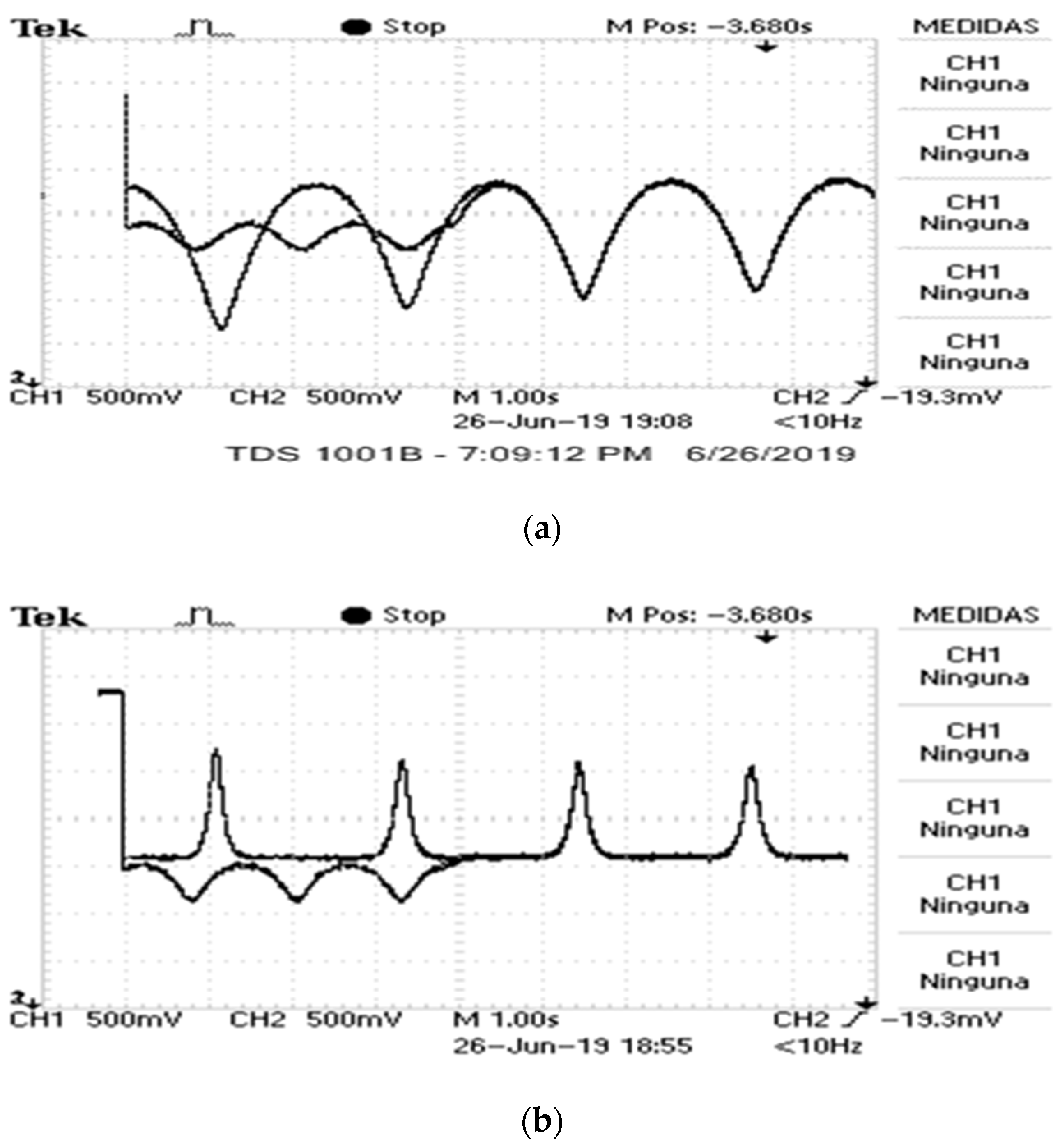
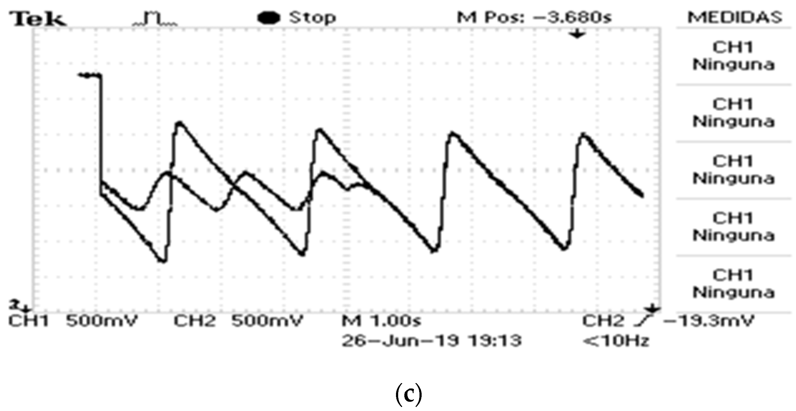
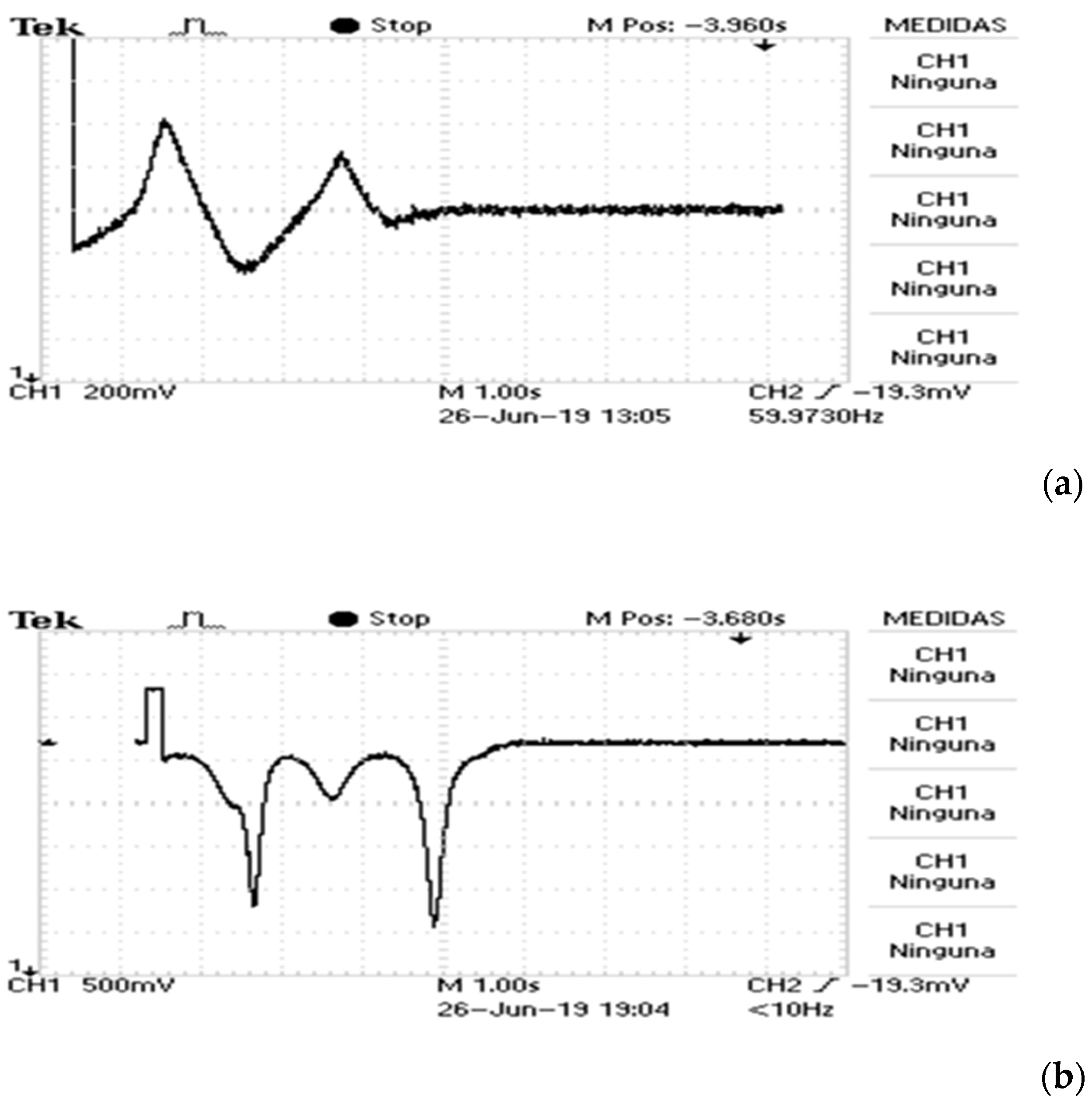
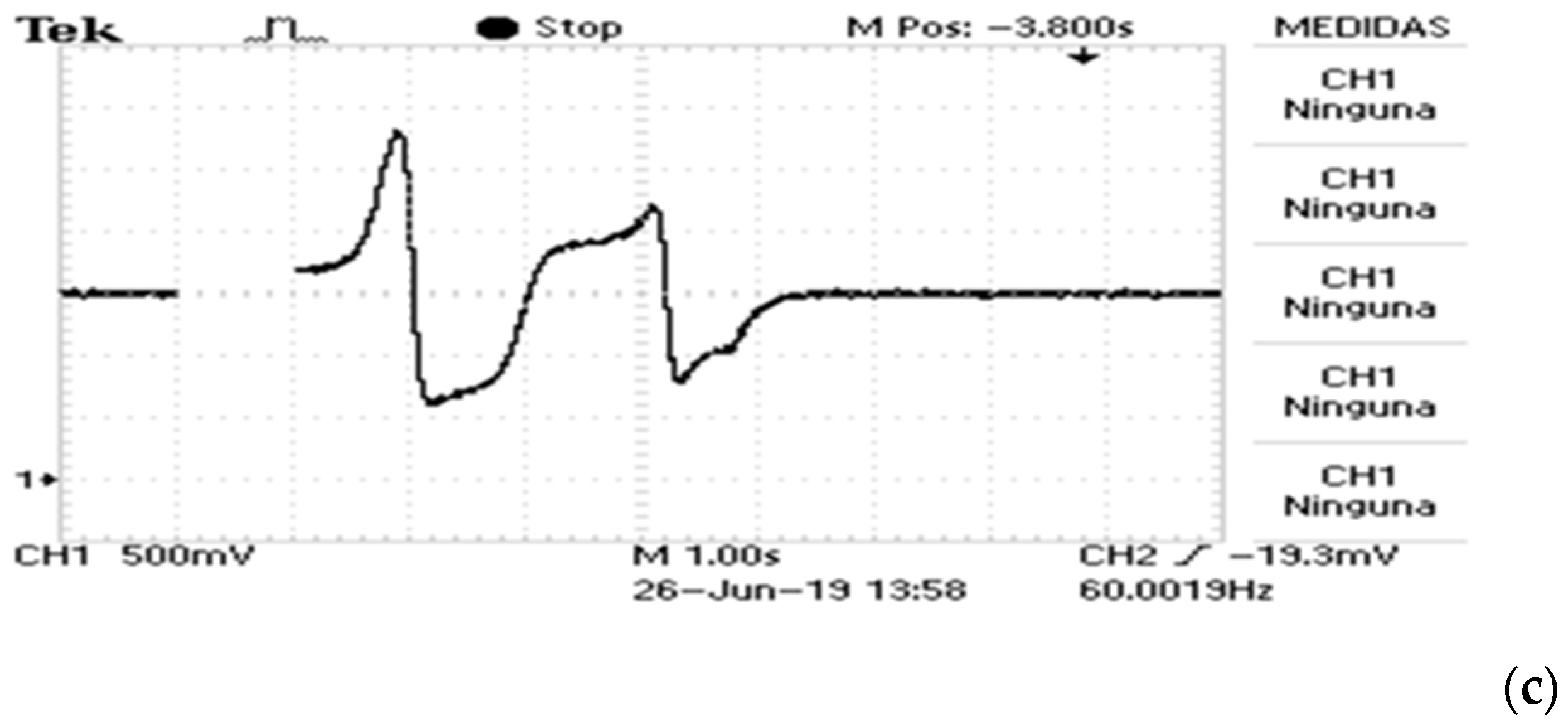
Experimental Results

As the digital to analog converter of the microcontroller has an operation range of $0.5$ to $2.7 \mathrm{V}$, the simulation and experimental results will be different in amplitude, except for states $x_m$ and $x_s$ whose values are inside the operating range of the microcontroller. If we want the same amplitude values that the numerical simulations, it would be necessary to add an external operational amplification stage for every state.

The state values of master and slave systems and synchronization error were scaled by software to avoid the amplification stage. The discrete Equations (21) remain the same, the values are only scaled before to be sent to the DAC’s to be seen in the oscilloscope, as it is shown in

Table 1. Scaling values of the experimental test using map function.

$o{x}_m\left(k\right)=map\left(x_m\left(k\right)\ast 1, -70.0, 21.0, 0.0, 4095.0\right)$

$o{x}_s\left(k\right)=map\left(x_s\left(k\right)\ast 1, -70.0, 21.0, 0.0, 4095.0\right)$

$o{y}_m\left(k\right)=map\left(y_m\left(k\right)\ast 10, -42.0, 50.6, 0.0, 4095.0\right)$

$o{y}_s\left(k\right)=map\left(y_s\left(k\right)\ast 10, -42.0, 50.6, 0.0, 4095.0\right)$

$o{z}_m\left(k\right)=map\left(z_m\left(k\right)\ast 40, -52.0, 52.0, 0.0, 4095.0\right)$

$o{z}_s\left(k\right)=map\left(z_s\left(k\right)\ast 40, -52.0, 52.0, 0.0, 4095.0\right)$

$o{e}_1\left(k\right)=map\left(e_1\left(k\right)\ast 50, -15.50, 22.0, 0.0, 4095.0\right)$

$o{e}_2\left(k\right)=map\left(e_2\left(k\right)\ast 20, -124.0, 00.0, 0.0, 4095.0\right)$

$o{e}_3\left(k\right)=map\left(e_3\left(k\right)\ast 60, -60.0, 86.4, 0.0, 4095.0\right)$

. In such a way, the equations in (21) are not modified. The scale value for each state or error is selected according to the minimum and maximum value obtained by simulation.

For the experimental tests, the next values were taking in account $a=12, b=0.4, r=1$ with initial conditions $x_m\left(0\right)= 0, y_m\left(0\right)= 0, z_m\left(0\right)= 0$ and $x_s\left(0\right)=-0.2, y_s\left(0\right)=-0.6, z_s\left(0\right)=0.2$. In Figure 8a–c the images of synchronization process are shown in a Tektronix TDS 1001B oscilloscope. During $t\le 4\mathrm{s}$ the behavior of both systems is different due to initial conditions, after $t>4 \mathrm{s}$ the synchronization process begins. The states $x_m$ and $x_s$ shown in Figure 8a has the same amplitude in experimental and numerical. The values of $y_m$, $y_s$ and $z_m$, $z_s$ are shown in Figure 8b,c, they do not have the same amplitude that values obtained by simulation, but they have the same behavior.

All signals have an offset due to the DAC operating range, it cannot be zero. The main idea of this experimental test is to see the feasibility to implement the active controller in a microcontroller, analyzing the synchronization behavior of the chaotic system and the performance of the active controller. For implementing the active controller in a real application, the offset produced by the DAC must be eliminated, and the state values of the chaotic differential equations must be scaled by using an external stage of operational amplifiers.

Finally, in Figure 9 is shown the behavior of the synchronization error obtained experimentally in the oscilloscope, by comparing this with the synchronization errors obtained in Figure 4 by simulation, it is possible to see that they have the same behavior, which implies that the synchronization process of the master-slave systems is achieved by the active control. The synchronization times after the control laws begin to work and the error values tend to zero are approximately $s{t}_{e_1}=1s; s{t}_{e_2}=0.8s; s{t}_{e_3}=0.9s$. Regarding to the time evolution of synchronization errors in Figure 9, all signals have offset due to the DAC operating range, the authors only placed the error signals in the center of the oscilloscope screen to see the behavior.

6. Conclusions

In this paper, an active controller was designed for the synchronization of the chaotic system of Petrzela. By using Lyapunov analysis, the exponential convergence to zero of the synchronization error was demonstrated. The gains used for $k_1,k_2 and k_3$ were selected by trial and error to guarantee system stability and, the feasibility of the controller was realized by numerical simulation and for the hardware implementation in a 32 bits ARM microcontroller. For future work, the controller can be optimized to find gains that do not compromise the speed of convergence with the magnitude of the input control.

References

1. Pecora, L.M.; Carroll, T.L. Synchronization in chaotic systems. Phys. Rev. Lett. 1990, 64, 821–825. [Google Scholar] [CrossRef] [PubMed]
2. Pecora, L.M.; Carroll, T.L.; Johnson, G.A.; Mar, D.J.; Heagy, J.F. Fundamentals of synchronization in chaotic systems, concepts, and applications. Chaos Int. J. Nonlinear Sci. 1997, 7, 520–543. [Google Scholar] [CrossRef] [PubMed] [Green Version]
3. Feki, M. An adaptive chaos synchronization scheme applied to secure communication. Chaos Solitons Fractals 2003, 18, 141–148. [Google Scholar] [CrossRef]
4. Tanougast, C.; Dandache, A.; Azzaz, M.S.; Sadoudi, S. Hardware design of embedded systems for security applications. In Embedded Systems—High Performance Systems, Applications and Projects; Intech: Rijeka Croatia, 2012; pp. 233–260. [Google Scholar]
5. Zapateiro De la Hoz, M.; Acho, L.; Vidal, Y. An experimental realization of a chaos-based secure communication using arduino microcontrollers. Sci. World J. 2015, 2015, 123080. [Google Scholar] [CrossRef] [PubMed]
6. Yang, T. A survey of chaotic secure communication systems. Int. J. Comput. Cognit. 2004, 2, 81–130. [Google Scholar]
7. Volos, C.K.; Kyprianidis, I.M.; Stouboulos, I.N. Image encryption process based on chaotic synchronization phenomena. Signal Proc. 2013, 93, 1328–1340. [Google Scholar] [CrossRef]
8. Nakamura, Y.; Sekiguchi, A. The chaotic mobile robot. IEEE Trans. Robot. Autom. 2001, 17, 898–904. [Google Scholar] [CrossRef]
9. Bae, Y.C.; Kim, J.W.; Kim, Y.G. Obstacle avoidance methods in the chaotic mobile robot with integrated some chaos equation. Int. J. Fuzzy Logic Intell. Syst. 2003, 3, 206–214. [Google Scholar] [CrossRef]
10. Fallahi, K.; Leung, H. A cooperative mobile robot task assignment and coverage planning based on chaos synchronization. Int. J. Bifurc. Chaos 2010, 20, 161–176. [Google Scholar] [CrossRef]
11. Fahmy, A.A. Performance evaluation of chaotic mobile robot controllers. Int. Trans. J. Eng. Manag. Appl. Sci. Technol. 2012, 3, 145–158. [Google Scholar]
12. Zang, X.; Iqbal, S.; Zhu, Y.; Liu, X.; Zhao, J. Applications of chaotic dynamics in robotics. Int. J. Adv. Robot. Syst. 2016, 13, 60. [Google Scholar] [CrossRef]
13. Volos, C.K.; Kyprianidis, I.M.; Stouboulos, I.N.; Nistazakis, H.E.; Tombras, G.S. Cooperation of autonomous mobile robots for surveillance missions based on hyperchaos synchronization. J. Appl. Math. Bioinf. 2016, 6, 125–143. [Google Scholar]
14. Campos, J.M.S. Inducción de trayectorias caóticas mediante acoplamiento de robots móviles para la cobertura de áreas específicas de forma síncrona. Ph.D. Thesis, Manufactura avanzada—CIATEQ, San Luis Potosí, México, January 2019. [Google Scholar]
15. Nasr, S.; Mekki, H.; Bouallegue, K. A multi-scroll chaotic system for a higher coverage path planning of a mobile robot using flatness controller. Chaos Solitons Fractals 2019, 118, 366–375. [Google Scholar] [CrossRef]
16. Lu, J.; Wu, X.; Han, X.; Lü, J. Adaptive feedback synchronization of a unified chaotic system. Phys. Lett. A 2004, 329, 327–333. [Google Scholar] [CrossRef]
17. Han, X.; Lu, J.A.; Wu, X. Adaptive feedback synchronization of Lü system. Chaos Solitons Fractals 2004, 22, 221–227. [Google Scholar] [CrossRef]
18. Wang, X.; Wang, Y. Adaptive control for synchronization of a four-dimensional chaotic system via a single variable. Nonlinear Dyn. 2011, 65, 311–316. [Google Scholar] [CrossRef]
19. Yang, C.C. Adaptive synchronization of Lü hyperchaotic system with uncertain parameters based on single-input controller. Nonlinear Dyn. 2011, 63, 447–454. [Google Scholar] [CrossRef]
20. Wang, F.; Liu, C. A new criterion for chaos and hyperchaos synchronization using linear feedback control. Phys. Lett. A 2006, 360, 274–278. [Google Scholar] [CrossRef]
21. Yan, Z.; Yu, P. Linear feedback control, adaptive feedback control and their combination for chaos (lag) synchronization of LC chaotic systems. Chaos Solitons Fractals 2007, 33, 419–435. [Google Scholar] [CrossRef]
22. Rafikov, M.; Balthazar, J.M. On control and synchronization in chaotic and hyperchaotic systems via linear feedback control. Commun. Nonlinear Sci. Numer. Simul. 2008, 13, 1246–1255. [Google Scholar] [CrossRef]
23. Chen, H.H. Chaos control and global synchronization of Liu chaotic systems using linear balanced feedback control. Chaos Solitons Fractals 2009, 40, 466–473. [Google Scholar] [CrossRef]
24. Huang, L.; Feng, R.; Wang, M. Synchronization of chaotic systems via nonlinear control. Phys. Lett. A 2004, 320, 271–275. [Google Scholar] [CrossRef]
25. Pérez-Cruz, J.H.; Portilla-Flores, E.A.; Niño-Suárez, P.A.; Rivera-Blas, R. Design of a nonlinear controller and its intelligent optimization for exponential synchronization of a new chaotic system. Optik 2017, 130, 201–212. [Google Scholar] [CrossRef]
26. Wang, Y.; Guan, Z.H.; Wang, H.O. Feedback and adaptive control for the synchronization of Chen system via a single variable. Phys. Lett. A 2003, 312, 34–40. [Google Scholar] [CrossRef]
27. Pérez-Cruz, J.H. Stabilization and Synchronization of Uncertain Zhang System by Means of Robust Adaptive Control. Complexity 2018, 2018, 4989520. [Google Scholar] [CrossRef]
28. Jiang, G.P.; Chen, G.; Tang WK, S. A new criterion for chaos synchronization using linear state feedback control. Int. J. Bifurc. Chaos 2003, 13, 2343–2351. [Google Scholar] [CrossRef]
29. Wu, X.; Cai, J.; Wang, M. Master-slave chaos synchronization criteria for the horizontal platform systems via linear state error feedback control. J. Sound Vib. 2006, 295, 378–387. [Google Scholar] [CrossRef]
30. Wu, X.; Chen, G.; Cai, J. Chaos synchronization of the master–slave generalized Lorenz systems via linear state error feedback control. Phys. D Nonlinear Phenom. 2007, 229, 52–80. [Google Scholar] [CrossRef]
31. Chen, Y.; Wu, X.; Gui, Z. Global synchronization criteria for a class of third-order non-autonomous chaotic systems via linear state error feedback control. Appl. Math Modell. 2010, 34, 4161–4170. [Google Scholar] [CrossRef]
32. Lin, Q.; Wu, X. The sufficient criteria for global synchronization of chaotic power systems under linear state-error feedback control. Nonlinear Anal. Real World Appl. 2011, 12, 1500–1509. [Google Scholar] [CrossRef]
33. Li, C.; Li, H. Robust control for a class of chaotic and hyperchaotic systems via linear state feedback. Phys. Scr. 2012, 85, 025007. [Google Scholar] [CrossRef]
34. Cruz, J.H.P.; Figueroa, M.; Paredes, S.A.R.; Villa, A.L. Synchronization of chaotic Akgul system by means of feedback linearization and pole placement. IEEE Latin Am. Trans. 2017, 15, 249–256. [Google Scholar] [CrossRef]
35. Shahverdiev, E.M.; Nuriev, R.A.; Hashimov, R.H.; Shore, K.A. Parameter mismatches, variable delay times and synchronization in time-delayed systems. Chaos Solitons Fractals 2005, 25, 325–331. [Google Scholar] [CrossRef] [Green Version]
36. Park, J.H.; Kwon, O.M. A novel criterion for delayed feedback control of time-delay chaotic systems. Chaos Solitons Fractals 2005, 23, 495–501. [Google Scholar] [CrossRef]
37. Emelianova, Y.P.; Emelyanov, V.V.; Ryskin, N.M. Synchronization of two coupled multimode oscillators with time-delayed feedback. Commun. Nonlinear Sci. Numer. Simul. 2014, 19, 3778–3791. [Google Scholar] [CrossRef] [Green Version]
38. Khan, A.; Budhraja, M.; Ibraheem, A. Multiswitching dual combination synchronization of time-delay chaotic systems. Math. Methods Appl. Sci. 2018, 41, 5679–5690. [Google Scholar] [CrossRef]
39. Varan, M.; Akgul, A. Control and synchronisation of a novel seven-dimensional hyperchaotic system with active control. Pramana 2018, 90, 54. [Google Scholar] [CrossRef]
40. Singh, P.P.; Roy, B.K. Comparative performances of synchronisation between different classes of chaotic systems using three control techniques. Ann. Rev. Control 2018, 45, 152–165. [Google Scholar] [CrossRef]
41. Vaidyanathan, S. Generalized projective synchronization of vaidyanathan chaotic system via active and adaptive control. In Advances and Applications in Nonlinear Control Systems; Springer: Cham, Switzerland, 2016; pp. 97–116. [Google Scholar]
42. Cicek, S.; Ferikoglu, A.; Pehlivan, I. A new 3D chaotic system: Dynamical analysis, electronic circuit design, active control synchronization and chaotic masking communication application. Optik 2016, 127, 4024–4030. [Google Scholar] [CrossRef]
43. Pérez, J.H. Neural control for synchronization of a chaotic Chua-Chen system. IEEE Latin Am. Trans. 2016, 14, 3560–3568. [Google Scholar] [CrossRef]
44. Jafari, S.; Sprott, J.C. Simple chaotic flows with a line equilibrium. Chaos Solitons Fractals 2013, 57, 79–84. [Google Scholar] [CrossRef]
45. Pham, V.T.; Jafari, S.; Volos, C.; Vaidyanathan, S.; Kapitaniak, T. A chaotic system with infinite equilibria located on a piecewise linear curve. Optik 2016, 127, 9111–9117. [Google Scholar] [CrossRef]
46. Jafari, S.; Sprott, J.C.; Pham, V.T.; Volos, C.; Li, C. Simple chaotic 3D flows with surfaces of equilibria. Nonlinear Dyn. 2016, 86, 1349–1358. [Google Scholar] [CrossRef]
47. Gotthans, T.; Petržela, J. New class of chaotic systems with circular equilibrium. Nonlinear Dyn. 2015, 81, 1143–1149. [Google Scholar] [CrossRef] [Green Version]
48. Nwachioma, C.; Pérez-Cruz, J.H. Realization and implementation of polynomial chaotic sun system. Phys. Sci. Int. J. 2017, 16, 1–7. [Google Scholar] [CrossRef]
49. Nwachioma, C.; Pérez-Cruz, J.H.; Jiménez, A.; Ezuma, M.; Rivera-Blas, R. A new chaotic oscillator-properties, analog implementation, and secure communication application. IEEE Access 2019, 7, 7510–7521. [Google Scholar] [CrossRef]
50. Rajagopal, K.; Cicek, S.; Pham, V.; Jafari, S.; Karthikeyan, A. A novel class of chaotic systems with different shapes of equilibrium and microcontroller-based cost-effective design for digital applications. Eur. Phys. J. Plus 2018, 133, 231. [Google Scholar] [CrossRef]
51. Giakoumis, A.E.; Volos, C.K.; Stouboulos, I.N.; Kyprianidis, I.K. Implementation of a hyperchaotic system with hidden attractors into a microcontroller. In Proceedings of the 20th International Conference on Circuits, Systems, Communications and Computers (CSCC 2016), Corfu Island, Greece, 14–17 July 2016. [Google Scholar]
52. Castañeda, C.E.; López-Mancilla, D.; Chiu, R.; Villafana-Rauda, E.; Orozco-López, O.; Casillas-Rodríguez, F.; Sevilla-Escoboza, R. Discrete-time neural synchronization between an Arduino microcontroller and a compact development system using multiscroll chaotic signals. Chaos Solitons Fractals 2019, 119, 269–275. [Google Scholar] [CrossRef]
53. Janakiraman, S.; Thenmozhi, K.; Rayappan, J.B.B.; Amirtharajan, R. Lightweight chaotic image encryption algorithm for real-time embedded system: Implementation and analysis on 32-bit microcontroller. Microprocess. Microsyst. 2018, 56, 1–12. [Google Scholar] [CrossRef]
54. Tlelo-Cuautle, E.; Rangel-Magdaleno, J.J.; Pano-Azucena, A.D.; Obeso-Rodelo, P.J.; Nunez-Perez, J.C. FPGA realization of multi-scroll chaotic oscillators. Commun. Nonlinear Sci. Numer. Simulat. 2015, 27, 66–80. [Google Scholar] [CrossRef]
55. Pano-Azucena, A.D.; Tlelo-Cuautle, E.; Rodriguez-Gomez, A.G.; de la Fraga, L.G. FPGA-based implementation of chaotic oscillators by applying the numerical method based on trigonometric polynomials. AIP Adv. 2018, 8, 075217. [Google Scholar] [CrossRef] [Green Version]
56. Tuna, M.; Fidan, C.B. Electronic circuit design, implementation and FPGA-based realization of a new 3D chaotic system with single equilibrium point. Optik 2016, 127, 11786–11799. [Google Scholar] [CrossRef]
57. Muthuswamy, B.; Banerjee, S. A Route to Chaos Using FPGAs; Springer: Cham, Switzerland, 2015. [Google Scholar]
Figure 1. (a) 3D projection of chaotic attractor system; (b) XY phase plane; (c) XZ phase plane; (d) YZ phase plane.
Computation 07 00040 g001
Figure 2. Chaotic attractor for master and slave systems; (a) 3D master attractor system; (b) 3D slave attractor system.
Computation 07 00040 g002
Figure 3. Synchronization process between master-slave systems by numerical simulation; (a) Synchronization process for first state; (b) Synchronization process for second state; (c) Synchronization process for third state.
Computation 07 00040 g003
Figure 4. Time evolution of synchronization error signals by numerical simulation e 1 ( t ) ,   e 2 ( t )   a n d   e 3 ( t ) .
Computation 07 00040 g004
Figure 5. Control signals u 1 ( t ) ,   u 2 ( t )   a n d   u 3 ( t ) .
Computation 07 00040 g005
Figure 6. Hardware of microcontroller based active controller implementation.
Computation 07 00040 g006
Figure 7. Flowchart of the active controller program.
Computation 07 00040 g007
Figure 8. Synchronization process between master-slave systems by experimental result; (a) Synchronization process for first state; (b) Synchronization process for second state; (c) Synchronization process for third state.
Computation 07 00040 g008aComputation 07 00040 g008b
Figure 9. Time evolution of synchronization error signals by experimental results; (a) synchronization error of e 1 ( t ) = x s x m ; (b) synchronization error of e 2 ( t ) = y s y m ; (c) synchronization error of e 3 ( t ) = z s z m .
Computation 07 00040 g009aComputation 07 00040 g009b