Clustering Improves the Goemans–Williamson Approximation for the Max-Cut Problem

 , , and
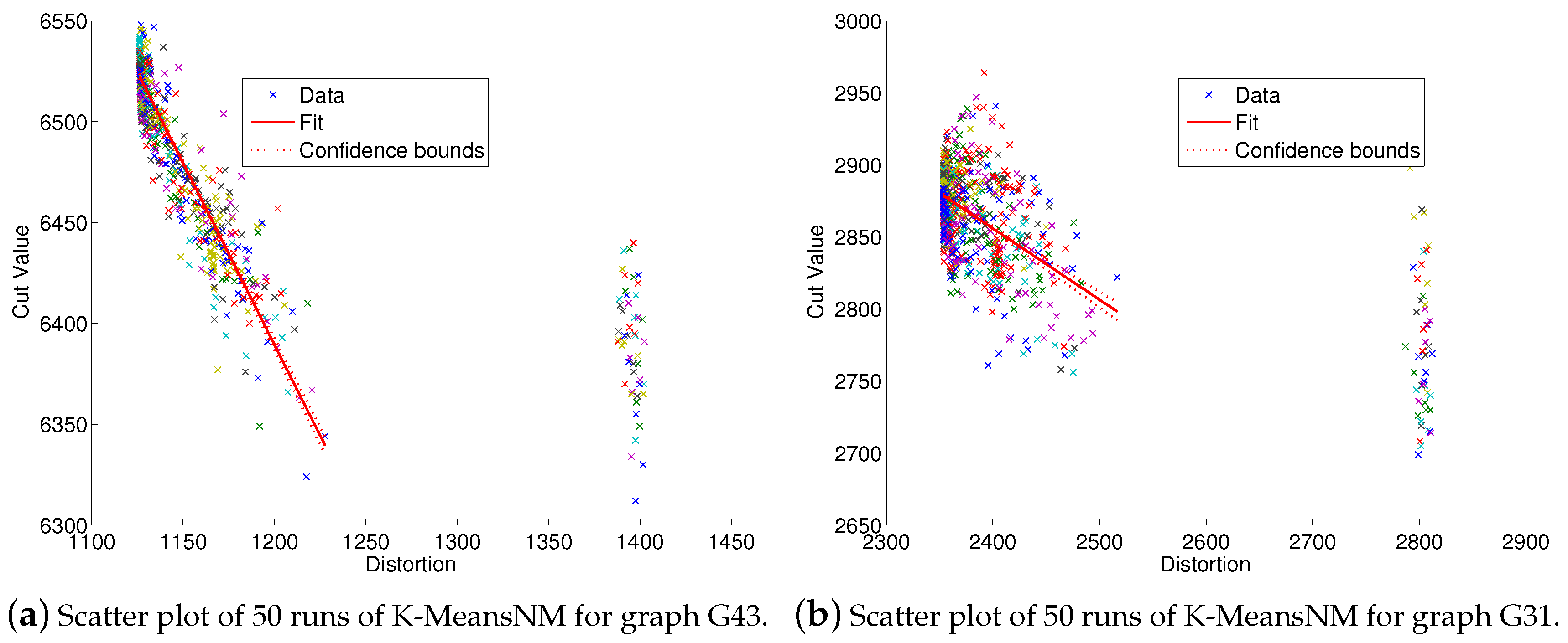
Abstract
:1. Introduction
2. Materials and Methods
2.1. Benchmark Data
2.2. Clustering in the Goemans–Williamson Algorithm
- Fuzzy c-means (Fuzzy)
- Randomized k-means initialized among vectors (K-MeansRand)
- Deterministic k-means (K-MeansDet)
- Randomized k-medoids (K-MedRand)
- Deterministic k-medoids (K-MedDet)
- Minimum Spanning Tree (MST)
- Randomized Rounding of Goemans–Williamson (RR)
- Randomized k-means initialized with two random vectors (K-Means2N)
- Randomized k-means initialized with a random vector and its negative (K-MeansNM)
2.3. Local Search
3. Results
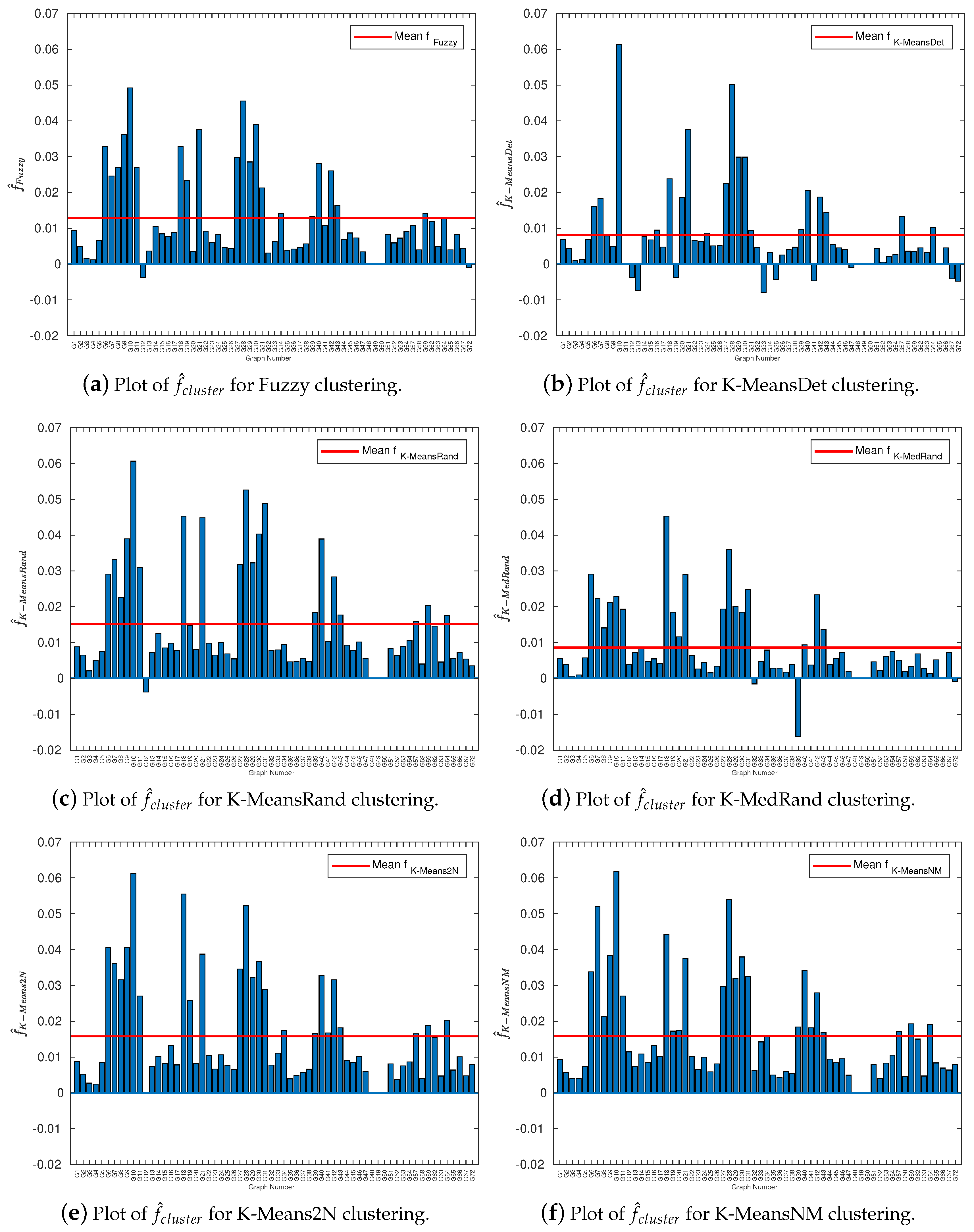
3.1. Cluster Quality Correlations with Solution Quality
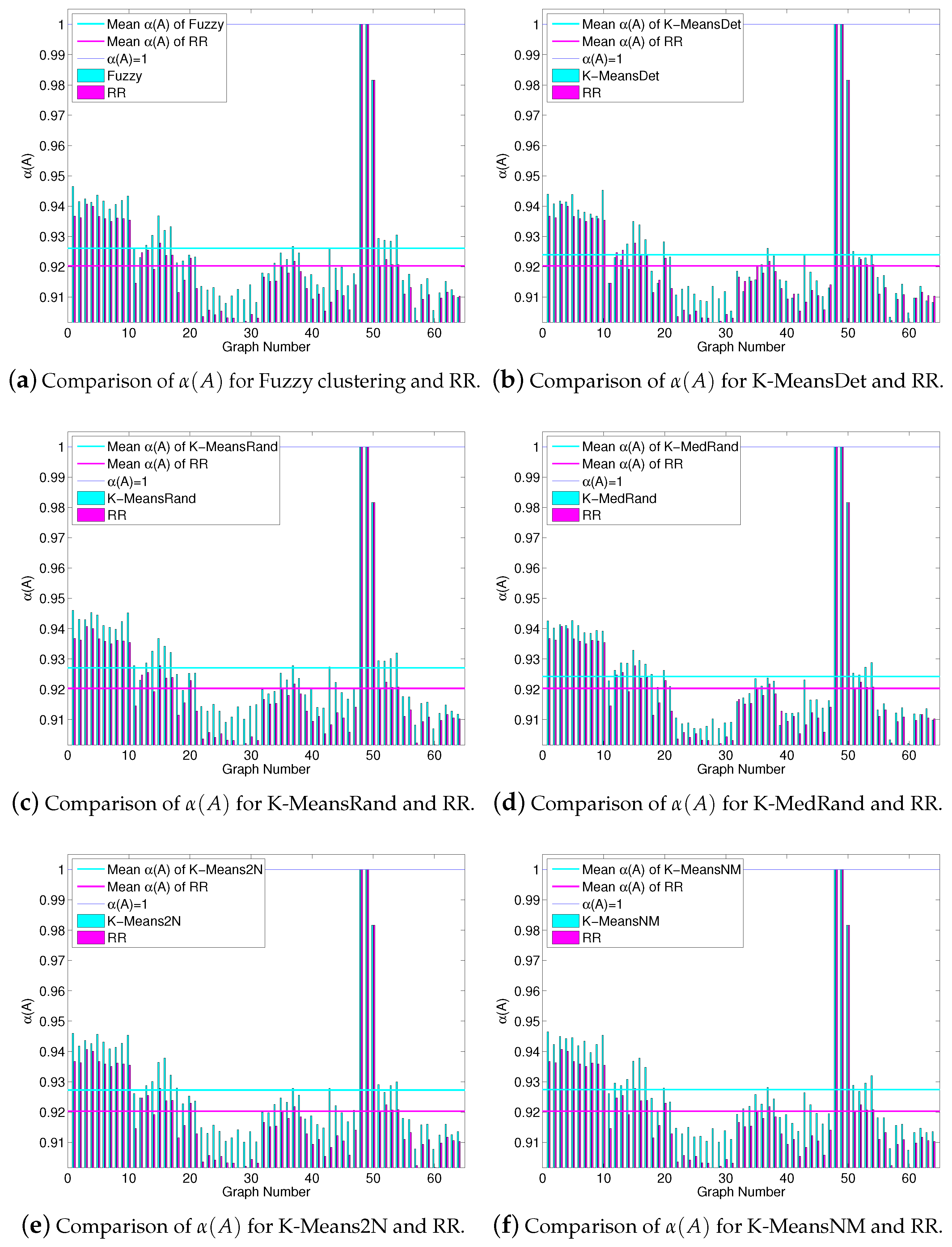
3.2. An Instance-Specific Approximation Guarantee
3.3. Benchmarking Experiments
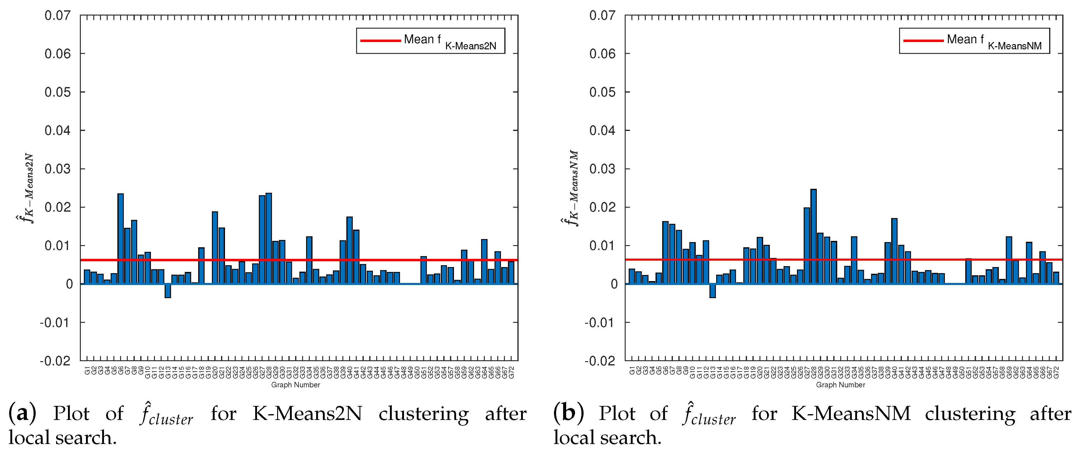
3.4. Local Search Improvement
4. Conclusions
Author Contributions
Funding
Acknowledgments
Conflicts of Interest
Abbreviations
| IQP | Integer Quadratic Programming |
| VP | Vector Programming |
| SDP | Semidefinite Programming |
| Fuzzy | Fuzzy c-means clustering |
| K-MeansRand | Randomized version of k-Means |
| K-MeansDet | Deterministic version of k-Means |
| K-MedRand | Randomized version of k-Medoids |
| K-MedDet | Deterministic version of k-Medoids |
| MST | Minimum Spanning Tree |
| RR | Randomized Rounding (Goemans–Williamson rounding) |
| K-Means2N | Randomized version of k-Means initialized with 2 random vectors |
| K-MeansNM | Deterministic version of k-Means initialized with a random vector and its negative |
References
- Karp, R.M. Reducibility among combinatorial problems. In Complexity of Computer Computation; Miller, R.E., Thacher, J.W., Eds.; Plenum Press: New York, NY, USA, 1972; pp. 85–103. [Google Scholar]
- Papadimitriou, C.H.; Yannakakis, M. Optimization, approximation, and complexity classes. J. Comput. Syst. Sci. 1991, 43, 425–440. [Google Scholar] [CrossRef] [Green Version]
- Hadlock, F. Finding a Maximum Cut of a Planar Graph in Polynomial Time. SIAM J. Comput. 1975, 4, 221–225. [Google Scholar] [CrossRef]
- Grötschel, M.; Nemhauser, G.L. A polynomial algorithm for the max-cut problem on graphs without long odd cycles. Math. Program. 1984, 29, 28–40. [Google Scholar] [CrossRef]
- Bodlaender, H.L.; Jansen, K. On the complexity of the maximum cut problem. Nord. J. Comput. 2000, 7, 14–31. [Google Scholar] [CrossRef]
- Anglès d’Auriac, J.C.; Preissmann, M.; Sebö, A. Optimal cuts in graphs and statistical mechanics. Math. Comput. Model. 1997, 26, 1–11. [Google Scholar] [CrossRef]
- Festa, P.; Pardalos, P.M.; Resende, M.G.C.; Ribeiro, C.C. Randomized heuristics for the Max-Cut problem. Optim. Methods Softw. 2002, 17, 1033–1058. [Google Scholar] [CrossRef]
- Klemm, K.; Mehta, A.; Stadler, P.F. Landscape Encodings Enhance Optimization. PLoS ONE 2012, 7, e34780. [Google Scholar] [CrossRef] [PubMed] [Green Version]
- Ma, F.; Hao, J.K. A multiple search operator heuristic for the max-k-cut problem. Ann. Oper. Res. 2017, 248, 365–403. [Google Scholar] [CrossRef] [Green Version]
- Shao, S.; Zhang, D.; Zhang, W. A simple iterative algorithm for maxcut. arXiv 2019, arXiv:1803.06496. [Google Scholar]
- Delorme, C.; Poljak, S. Laplacian eigenvalues and the maximum cut problem. Math. Program. 1993, 62, 557–574. [Google Scholar] [CrossRef]
- Poljak, S.; Rendl, F. Solving the max-cut problem using eigenvalues. Discret. Appl. Math. 1995, 62, 249–278. [Google Scholar] [CrossRef] [Green Version]
- Trevisan, L. Max Cut and the Smallest Eigenvalue. SIAM J. Comput. 2012, 41, 1769–1786. [Google Scholar] [CrossRef] [Green Version]
- Soto, J.A. Improved Analysis of a Max-Cut Algorithm Based on Spectral Partitioning. SIAM J. Discret. Math. 2015, 29, 259–268. [Google Scholar] [CrossRef] [Green Version]
- Goemans, M.X.; Williamson, D.P. Improved approximation algorithms for maximum cut and satisfiability problems using semidefinite programming. J. ACM 1995, 42, 1115–1145. [Google Scholar] [CrossRef]
- Grippo, L.; Palagi, L.; Piccialli, V. An unconstrained minimization method for solving low-rank SDP relaxations of the maxcut problem. Math. Program. 2011, 126, 119–146. [Google Scholar] [CrossRef]
- Palagi, L.; Piccialli, V.; Rendl, F.; Rinaldi, G.; Wiegele, A. Computational Approaches to Max-Cut. In Handbook on Semidefinite, Conic and Polynomial Optimization; Springer: Boston, MA, USA, 2011; pp. 821–847. [Google Scholar] [CrossRef] [Green Version]
- Mahajan, S.; Ramesh, H. Derandomizing semidefinite programming based approximation algorithms. In Proceedings of the IEEE 36th Annual Foundations of Computer Science, Milwaukee, WI, USA, 23–25 October 1995; pp. 162–169. [Google Scholar] [CrossRef]
- Håstad, J. Some optimal inapproximability results. J. ACM 2001, 48, 798–859. [Google Scholar] [CrossRef]
- Khot, S.; Kindler, G.; Mossel, E.; O’Donnell, R. Optimal inapproximability results for MAX-CUT and other 2-variable CSPs? SIAM J. Comput. 2007, 37, 319–357. [Google Scholar] [CrossRef] [Green Version]
- Feige, U.; Karpinski, M.; Karpinski, M. Improved approximation of Max-Cut on graphs of bounded degree. J. Algorithms 2002, 43, 201–219. [Google Scholar] [CrossRef]
- MacQueen, J. Some methods for classification and analysis of multivariate observations. In Proceedings of the Fifth Berkeley Symposium on Mathematical Statistics and Probability, Volume 1: Statistics; University of California Press: Berkeley, CA, USA, 1967; Volume 1, pp. 281–297. [Google Scholar]
- Dhillon, I.S.; Modha, D.S. Concept Decompositions for Large Sparse Text Data Using Clustering. Mach. Learn. 2001, 42, 143–175. [Google Scholar] [CrossRef] [Green Version]
- Kaufmann, L.; Rousseeuw, P. Clustering by Means of Medoids. In Data Analysis Based on the L1-Norm and Related Methods; Dodge, Y., Ed.; North-Holland: Amsterdam, The Netherlands, 1987; pp. 405–416. [Google Scholar]
- Bezdek, J.C. Pattern Recognition with Fuzzy Objective Function Algorithms; Springer: Boston, MA, USA, 1981. [Google Scholar] [CrossRef]
- Grygorash, O.; Zhou, Y.Z.; Jorgensen, Z. Minimum Spanning Tree Based Clustering Algorithms. In Proceedings of the 18th IEEE International Conference on Tools with Artificial Intelligence (ICTAI’06), Arlington, VA, USA, 13–15 November 2006; Lu, C.T.L., Bourbakis, N.G.B., Eds.; IEEE Computer Society: Los Alamitos, CA, USA, 2006; pp. 73–81. [Google Scholar] [CrossRef]
- Bishop, C.M. Pattern Recognition and Machine Learning (Information Science and Statistics); Springer: Berlin/Heidelberg, Germany, 2006. [Google Scholar]
- Hastie, T.; Tibshirani, R.; Friedman, J. The Elements of Statistical Learning: Data Mining, Inference, and Prediction; Springer: Berlin/Heidelberg, Germany, 2009. [Google Scholar]


© 2020 by the authors. Licensee MDPI, Basel, Switzerland. This article is an open access article distributed under the terms and conditions of the Creative Commons Attribution (CC BY) license (http://creativecommons.org/licenses/by/4.0/).
Share and Cite
Rodriguez-Fernandez, A.E.; Gonzalez-Torres, B.; Menchaca-Mendez, R.; Stadler, P.F. Clustering Improves the Goemans–Williamson Approximation for the Max-Cut Problem. Computation 2020, 8, 75. https://0-doi-org.brum.beds.ac.uk/10.3390/computation8030075
Rodriguez-Fernandez AE, Gonzalez-Torres B, Menchaca-Mendez R, Stadler PF. Clustering Improves the Goemans–Williamson Approximation for the Max-Cut Problem. Computation. 2020; 8(3):75. https://0-doi-org.brum.beds.ac.uk/10.3390/computation8030075
Chicago/Turabian StyleRodriguez-Fernandez, Angel E., Bernardo Gonzalez-Torres, Ricardo Menchaca-Mendez, and Peter F. Stadler. 2020. "Clustering Improves the Goemans–Williamson Approximation for the Max-Cut Problem" Computation 8, no. 3: 75. https://0-doi-org.brum.beds.ac.uk/10.3390/computation8030075