Article

Identifying Potential Machine Learning Algorithms for the Simulation of Binding Affinities to Molecularly Imprinted Polymers

1
Sensor Engineering Department, Faculty of Science and Engineering, Maastricht University, P.O. Box 616, 6200 MD Maastricht, The Netherlands
2
Maastricht Science Programme, Faculty of Science and Engineering, Maastricht University, P.O. Box 616, 6200 MD Maastricht, The Netherlands
*
Author to whom correspondence should be addressed.
Submission received: 13 August 2021 / Revised: 10 September 2021 / Accepted: 23 September 2021 / Published: 24 September 2021
(This article belongs to the Section Computational Chemistry)

Abstract

:
Molecularly imprinted polymers (MIPs) are synthetic receptors engineered towards the selective binding of a target molecule; however, the manner in which MIPs interact with other molecules is of great importance. Being able to rapidly analyze the binding of potential molecular interferences and determine the selectivity of a MIP can be a long tedious task, being time- and resource-intensive. Identifying computational models capable of reliably predicting and reporting the binding of molecular species is therefore of immense value in both a research and commercial setting. This research therefore sets focus on comparing the use of machine learning algorithms (multitask regressor, graph convolution, weave model, DAG model, and inception) to predict the binding of various molecular species to a MIP designed towards 2-methoxphenidine. To this end, each algorithm was “trained” with an experimental dataset, teaching the algorithms the structures and binding affinities of various molecular species at varying concentrations. A validation experiment was then conducted for each algorithm, comparing experimental values to predicted values and facilitating the assessment of each approach by a direct comparison of the metrics. The research culminates in the construction of binding isotherms for each species, directly comparing experimental vs. predicted values and identifying the approach that best emulates the real-world data.

1. Introduction

In recent decades, advancements in the field of biosensing have precipitated the development of point-of-care (PoC) technologies for the rapid analysis of a whole host of molecules [1,2]. The main driving force behind these marvels lies in the advancement of the receptor materials utilized in the transduction of a biological/chemical target into a tangible output signal [3]. Molecularly imprinted polymers (MIPs) are a primary example of a developed synthetic receptor material, consisting of a highly crosslinked polymeric network with selective nanocavities engineered for the binding of an analyte distributed throughout [4,5]. These synthetic alternatives to biological recognition elements demonstrate enhanced resistance to extreme physical conditions and can operate in a wide range of scenarios, which is highlighted in the increasing number of applications that have been linked to these synthetic wonders [6].
Traditionally, MIPs have been developed through a time-consuming trial-and-error methodology consisting of altering the chemical compositions and ratios of the monomer and crosslinker species to achieve desired results [7,8]. The same tedium exists for determining the performance of a MIP, having to expose it to countless molecular moieties to truly determine the selective capabilities of the polymer [9,10]. Due to the nature of PoC analysis, this testing process is vital, though traditional approaches have proven costly and protracted. The potential to lessen these constrictors does exist and lies within the realms of data science, more commonly referred to as computational chemistry. Many chemical processes have already benefited from the implementation of diverse algorithms, revolutionizing the fields of retrosynthesis, reaction optimization, and drug design [11,12,13]. Computational methods have also been applied to molecularly imprinted polymers, though they focus on the compositional nature rather than the binding of various analytes [14,15,16,17].
One computational tool that can aid the development of MIPs is machine learning, and in particular the use of neural networks (NN). This kind of machine learning methodology is most commonly applied in the fields of chemo-informatics, enabling the prediction of the physical and chemical properties of molecules, or even how a compound is likely to react [18,19,20]. As more datasets on molecules have become available, the use of NN has become increasingly more popular, with this approach offering more reliable chemical predictions [21,22]. This success can be derived from the different NN architectures possible, enabling chemical information to be layered and processed in numerous ways that allow new trends and relationships to be perceived [23]. The dataset and desired outcomes of analysis dictate which model is selected, though the selection may not have an obvious choice and requires investigation.
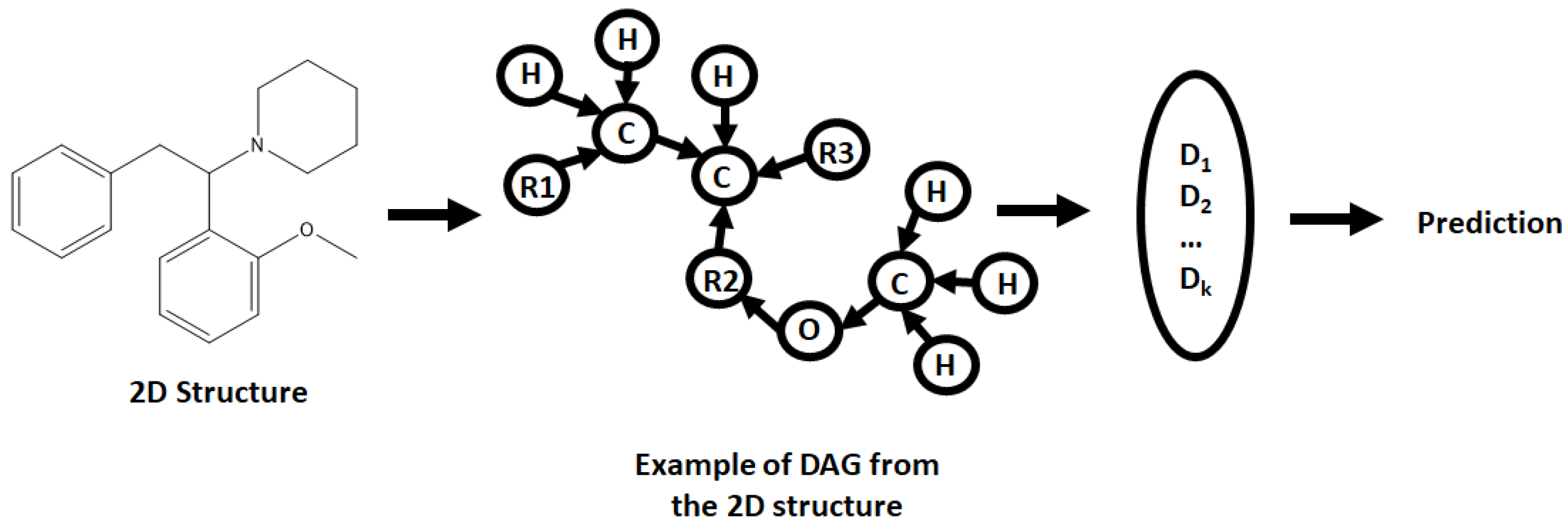
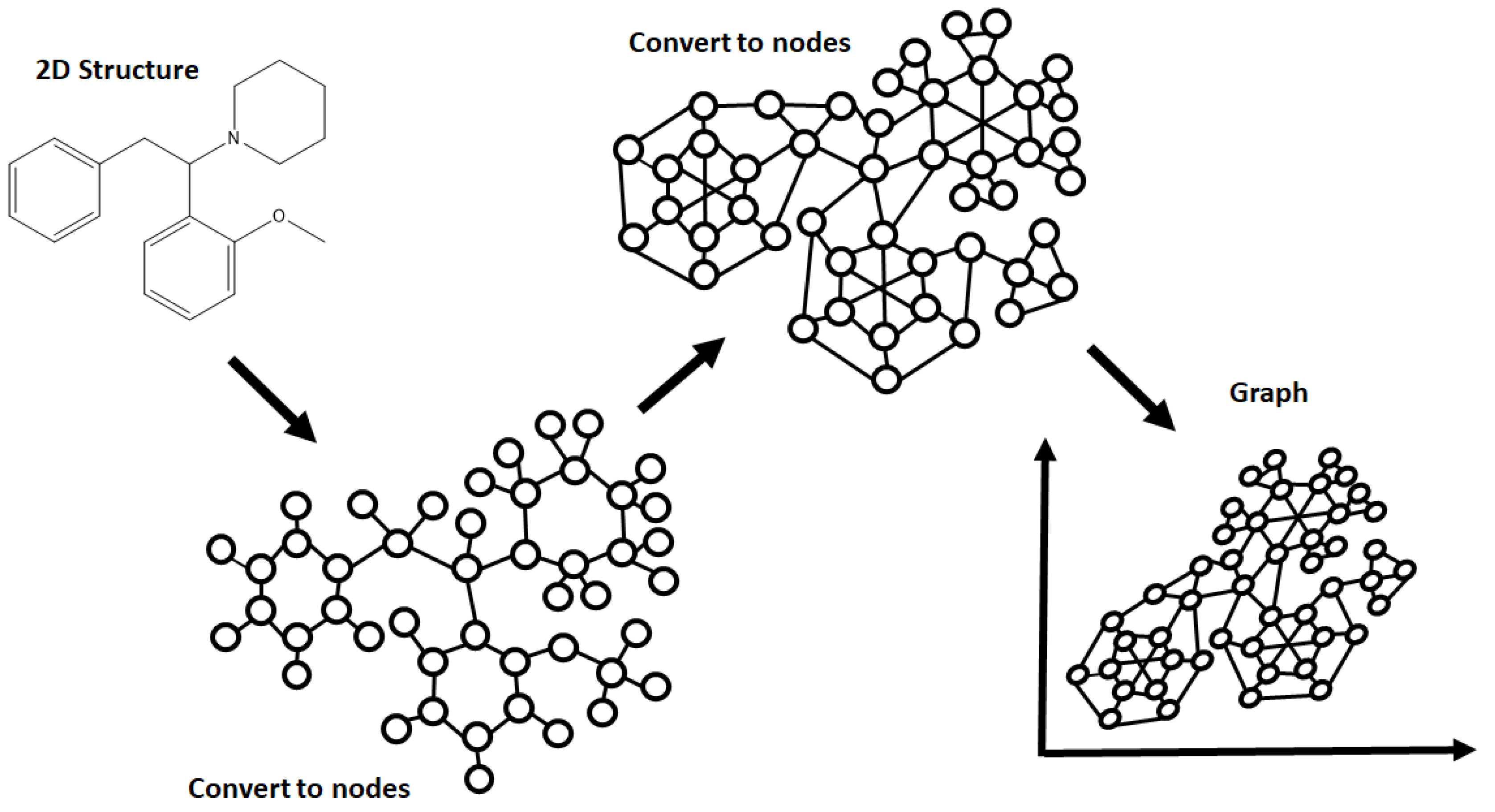
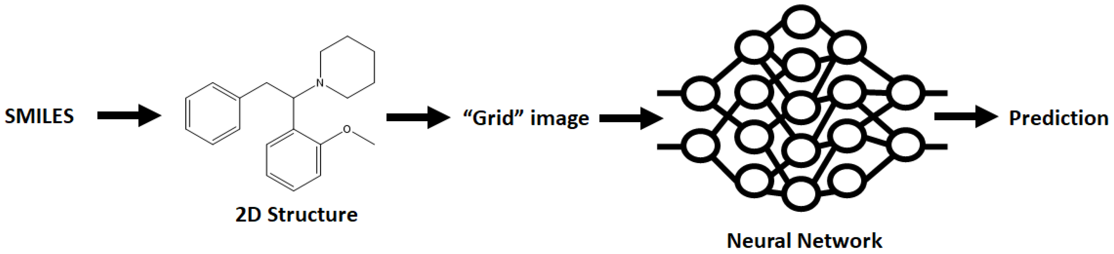
A wide range of NN architectures has been documented, including Directed Acyclic Graphs (DAG), Spatial Graph convolution, Multitask Regressors, and image classification models, to name just a few [24,25,26,27]. Each has a unique manner in which it processes data, though all require molecular structures and other variables to be preprocessed prior to analysis. This preprocessing is known as featurizing, a process that can also affect the way the model selected interprets the data [28,29]. Molecular structures are featurized by converting them into Simplified Molecular Input Line Entry Specification (SMILES), transforming a molecular structure into a line of text that the models can interpret [30]. The manner in which the rest of the data (including the SMILES) is featurized depends on the model selected, adding to the complexity of model selection. All in all, the best method of selecting a model is a trial and error approach, attempting different models and selecting the best performing as a basis to be built upon.
Due to the complex nature of NN, knowledge in the field is critical for success. As the field of neural networking has expanded, an increasing number of research groups in many different areas has adopted these algorithms for data analysis, making the demand for experts in NN higher than ever before [31]. This increase in demand has led to the development of deep learning frameworks such as DeepChem that offer a host of deep learning architectures that can be modified and used with little experience [32,33,34]. DeepChem is a python-based framework that specifically targets chemistry, offering deep learning algorithms tailored towards the analysis of molecular datasets, thus making it a perfect platform for building and testing molecular NN models for the analysis and prediction of MIP binding behavior.
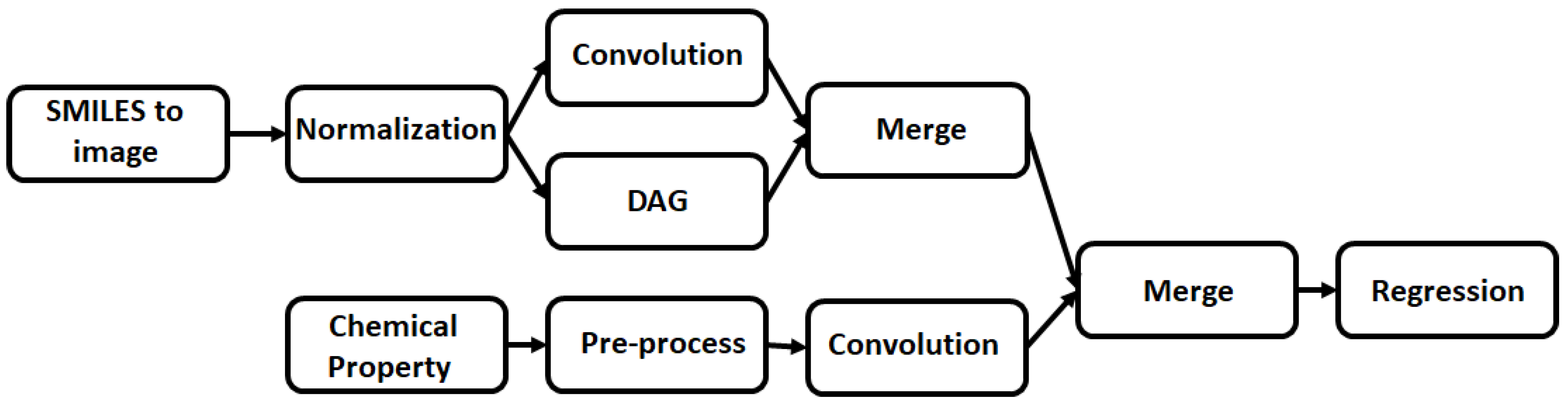
The presented research sets focus on using this framework to evaluate which model and featurizer simulates best the binding of specific substrates to a MIP when compared to real world data. To this end, four different featurizers were utilized in the modelling of this data: the RDKitDescriptors, weave featurizer, ConvMolFeaturizer, and the SmilesToImage featurizers. The featurized datasets were then coupled to three different NN models: the Directed Acyclic Graph (DAG) model, Graph Convolution model, and multitask regressor. These models were trained and tested with a combination of data from previous publications and data collected specifically for the purpose of this publication.

2. Dataset Selection

Over the years, MIPs have been applied to the detection of many different small molecules, demonstrating how they can be used as synthetic receptors in many different fields [35]. A lot of data therefore exists in regard to different compositions of MIPs with a corresponding template. The data however lack depth, with specific MIP binding data generally only extending towards the template molecule and a few analogues/interferants [36]. Finding datasets that provide a sufficient amount of molecular species binding to a MIP is therefore a tricky task.
An area where extensive binding data is of high importance is the field of drug screening. This area has seen a surge of activity in recent years with the “umbrella” of illicit substances being expanded to encompass new chemical architectures beyond classical drugs of abuse [37]. This extended prohibition now covers compounds coined New Psychoactive Substances (NPS), being compounds that are synthetically modified variants of classical compounds that contain a psychoactive pharmacophore with an overall different chemical architecture [38]. A prime example of such a compound is 2-methoxphenidine (2-MXP). Being akin to the classical compounds ketamine and phencyclidine (PCP), 2-MXP acts on the NMDA receptors and has dissociative effects on the user [39]. Other positional isomers of the compound exist, and current preliminary test methodologies can easily mistake the compound for a whole variety of compounds, including caffeine, which is not controlled [40]. It is therefore key to have binding data that covers a large array of molecules for sensors designed for these kinds of compounds, as false positives/negatives have become a greater issue as chemical architectures stray away from the norm.
With this in mind, the data selected for the training and testing of the generated neural network models are derived from the NPS field. With the research groups’ prior experience in this area, there is already MIP based data covering a range of chemical structures that can be used for training and test the models. The data were compiled from multiple NPS-based papers [41,42] and unpublished results to produced datasets for the training of the models. This training set was randomly selected from the data collected from the sources, introducing the models to a variety of structures in a bid to increase the models’ recognition of a diverse range of molecules. Each molecule introduced has a corresponding SMILES, initial concentration of substrate (Ci), amount of substrate bound to the MIP at equilibrium (Sb), and amount of substrate remaining in solution at equilibrium (Cf). The same was true for the testing dataset, though the number of molecules for this was dramatically reduced, as the bulk of the molecular data was used for the training of the models.
The following research therefore outlines the methods used to train and test models based on specific algorithms, evaluating these models using statistical techniques (R2, Pearson R2, and MAE score), alongside comparing the predicted values to those of the experimental data. Overall, the research endeavored to identify which of the algorithms are the most promising towards modelling MIP binding affinities based on limited datasets.

3. Modelling Methodology

3.1. Hardware and Software

All computational modelling and calculations were conducted on a desktop system (components and technical specifications: CPU—AMD Ryzen 7 3700x, MSI B550-A Pro motherboard ATX, 16 Gb DDR 4, 1 TB M.2 SSD, GPU—GeForce RTX 3070 OC 8 G, 850 W power supply) installed with Windows 10. Models and featurizers from DeepChem framework (with TensorFlow GPU enabled) were used for model training and testing, utilizing Jupyter Notebook to run the calculations, and data analysis was conducted with the NumPy package. The collected data was then plotted with OriginPro (2020 edition).

3.2. Datasets

All the data used in the training and testing of the computational models were gathered from previous publications or are unpublished data gathered with the distinct purpose of further characterizing the binding affinities of the selected MIP [41,42]. The MIP binding affinities for 2-MXP, 3-MXP, 4-MXP, caffeine, 2-MEPE, 3-MEPE, 4-MEPE, diphenidine, ephenidine, phenol red, crystal violet, malachite green, basic blue, paracetamol, aspirin, methyl orange, and sucrose were derived from these papers. The corresponding NIP data were collected to compliment these datapoints and to provide reference data for the computational models for comparison.
For the “training” of the NN models a dataset consisting of binding capacities (Sb) and free concentrations (Cf) at defined initial concentrations (Ci) for a variety of molecular species towards the target MIP was presented (see Supplementary Information Table S1). The molecular data in this training set were represented by the corresponding SMILES of each molecule, with this field being the primary featurized component of the data. Each model was then trained towards the prediction of the Sb and corresponding Cf at defined Ci values (0.1–0.5 mM). The same process was also completed for the corresponding MIP data to act as a reference (see Supplementary Information Table S2)
Three molecules were selected for the testing of the models, consisting of 3-methoxphenidine, diphenidine, and 3-methoxyephendine. The molecules selected were structural analogues of molecules in the training set, and were expected provide a valid metric of determining whether the models were performing sufficiently. As with the training set, the Sb and Cf values at defined Ci were determined and compared to the collected experimental values (see Supplementary Information Table S3). The same process was also completed for the corresponding MIP data to act as a reference (see Supplementary Information Table S4).

3.3. Directed Acyclic Graph (DAG) Model

An initial step of preprocessing the molecular data into a DAG compatible format was required, converting molecular structures into nodes/vertices (atoms) and edges (bonds) (Figure 1). This was achieved by processing the initial data frames with a DAG transformer, producing said vertices and edges for each molecule. As the graphs generated were acyclic, the orientation and direction of the graphs had been defined; therefore, all vertices were cycled through, designating each one vertex in turn the root of the graph. All other remaining vertices and edged were then direct towards the selected root, producing the DAG (example given in Figure 1, for the 2-methoxphenidine). As the data were built around the binding of simple molecules, it is feasible that a DAG can be generated for each atom within the molecule within a reasonable timeframe. In short, if a molecule has N vertices correlated with N atoms it will produce N DAG [43].
Each node (ν) has an associated contextual vector (Gν,k) indexed by k (the associated DAG). Gν,k correlates information about a corresponding atom and its neighbors (or parent vertices (pa1ν,k, …, panν,k)), with an input vector i and a function MG that implements recursion (Equation (1)) based on other parameters selected for the neural network [43]. The sum from each of the generated DAGs are then combined, producing a DAG-RNN (DAG–recursive neural network), relating all the information and producing an output value.
G ν , k =   M G ( i v ,   G pa [ ν ,   k ] 1 ,   , G pa [ ν ,   k ] n )
This model was constructed using the model builder in the DeepChem framework, training the model dataset using the default parameters settings (max_atoms = 50, n_atom_feat = 75, n_graph_feat = 30, n_outputs = 30, layer_sizes = [100], layer_sizes_gather = [100], dropout = none, model = regression, n_classes = 2), before using the basic model for parameter optimization. Hyperparameter optimization was conducted using a grid approach, determining the optimum model across a range of parameters (Appendix A) basing the optimum values off the generated R2 and Pearson R2 metrics. These parameters were analyzed across a range (10–1200) of epochs (iterations) to determine the optimum number of iterations to avoid over training of the model. The optimized model was then used to predict the Sb and corresponding Cf values at defined Ci values for the testing dataset. These values were then plotted alongside their experimental counterparts to produce a comparative binding isotherm.

3.4. Graph Convolution Model

Similar to DAG, the graph convolution model has the ability to represent a molecular structure as vertices (atoms) and edges (bonds) (Figure 2). The main difference lies in how the layers of the model are processed, with the model taking the product of translated functions (known as convolution) to extrapolate extra information or to find more complex patterns within the given data. At the lower levels of the network the same filter (convolution) is applied to neighboring atoms and bonds, with the information learned being combined after several steps generating a global pool that represents larger chunks of the network. The process can then be repeated for the higher levels, finding more relationships within the data and building a model of greater complexity [44].
This model was constructed using the model builder in the DeepChem framework, training the model dataset using the default parameters settings (number_atom_features = 75, graph_conv_layers = [64, 64], dense_layer_size = 128, dropout = none, model = regression, n_classes = 2), before using the basic model for parameter optimization. Hyperparameter optimization was conducted using a grid approach, determining the optimum model across a range of parameters (Appendix A) basing the optimum values of the generated R2 and Pearson R2 metrics. These parameters were analyzed across a range (10–1200) of epochs (iterations) to determine the optimum number of iterations to avoid over training of the model. The optimized model was then used to predict the Sb and corresponding Cf values at defined Ci values for the testing dataset. These values were then plotted alongside their experimental counterparts to produce a comparative binding isotherm.

3.5. Graph Convolution Weave Model

A different variant of the graph convolution model exists, consolidating primitive operations between atoms and their corresponding layers into a single module. Thus, rather than finding correlations in big chunks of data, the model finds links between smaller chunks going back and forth in nature. The back and forth nature of the learned relationships giving rise to the coined name “weave” convolution. The degree to which the data is weaved can easily be controlled by limiting the amount of “back and forth” data processing that occurs, with over iteration of this process having negative effects on the learned data. This methodology therefore has appeal, as it has the potential to produce more informative representations of the original input, and enables the option of stacking weave modules with limited atom pairs to produce more in-depth models [45].
As with the other models, the model was constructed using the DeepChem framework model builder, training the model data using the default parameter settings (n_atom_feat = 75, n_pair_feat = 14, n_hidden = 50, n_graph_feat = 128, n_weave = 2, fully_connected_layer_sizes = [2000, 100], conv_weight_init_stddevs = 0.03, weight_init_stddevs = 0.01, dropouts = 0.25, mode = regression) before using the basic model for parameter optimization. Hyperparameter optimization was conducted using a grid approach, determining the optimum model across a range of parameters (Appendix A) basing the optimum values off the generated R2 and Pearson R2 metrics. These parameters were analyzed across a range (10–1200) of epochs (iterations) to determine the optimum number of iterations to avoid over training of the model. The optimized model was then used to predict the Sb and corresponding Cf values at defined Ci values for the testing dataset. These values were then plotted alongside their experimental counterparts to produce a comparative binding isotherm.

3.6. Multitask Regressor Model

A multitask regressor approach would enable the training of multiple targets with the same input features, e.g., to classify/regress a molecule on both its 2D chemical structure and associated chemical properties. This means the model has more than one input that the model handles simultaneously and can be used to predict the regression product (Figure 3) [46]. This could be ideal for the analysis of molecular interactions with MIPs, as there are multiple chemical properties that can be factored into the model, producing more detailed and comprehensive predictions.
To this end, the RdKit descriptors were selected that could take the molecular SMILE and compute a list of chemical descriptors that are relevant to the selected molecule, e.g., molecular weights, number of valence electrons, partial charge, size, etc. [47]. This information was then used to featurize the experimental binding data to train the regressor model. To this end the DeepChem framework model builder was utilized for model training and testing using default parameters (n_features = 208, layer_sizes = [1000, 1000, 1000], dropout = 0.2, learn_rate = 0.0001) before using this base model for optimization. Hyperparameter optimization was conducted using a grid approach, determining the optimum model across a range of parameters (Appendix A) basing the optimum values off the generated R2 and Pearson R2 metrics. These parameters were analyzed across a range (10–1200) of epochs (iterations) to determine the optimum number of iterations to avoid over training of the model. The optimized model was then used to predict the Sb and corresponding Cf values at defined Ci values for the testing dataset. These values were then plotted alongside their experimental counterparts to produce a comparative binding isotherm.

3.7. ChemCeption Model

An alternative method of data analysis is possible by using the ChemCeption model of molecular analysis where a 2D structure of the molecule is generated from the SMILES, which in turn is mapped onto an array and used to train a neural network. The method essentially uses the 2D image of the molecule and breaks it down into a pixel grid which then has the measured chemical properties associated with it and a neural network generated that is trained towards the likeness of molecular structures (Figure 4). This simplistic approach bypasses a lot of other chemical characteristics that the other methods employ, though this technique has proven to be effective in other areas of cheminformatics.
As with the other algorithms, the model was constructed using the DeepChem framework model builder, training the model using the default parameter settings (img_spec = std, img_size = 80, base_filters = 16, inception_blocks = dict, n_classes = 2, mode = regression) before using the basic model for parameter optimization. As the model relies upon the transforming of an image into a neural network, a SMILES to image featurizer was utilized prior to the training and testing of the model data. Hyperparameter optimization was conducted using a grid approach, determining the optimum model across a range of parameters (Appendix A) basing the optimum values off the generated R2 and Pearson R2 metrics. These parameters were analyzed across a range (10–1200) of epochs (iterations) to determine the optimum number of iterations to avoid over training of the model. The optimized model was then used to predict the Sb and corresponding Cf values at defined Ci values for the testing dataset. These values were then plotted alongside their experimental counterparts to produce a comparative binding isotherm.

4. Results and Discussion

4.1. Direct Acyclic Graph (DAG) Model (ConvMolFeaturizer)

After optimization of the DAG model, it was trained at each Ci value individually, recording the MAE score, R2, Pearson R2, and RMS for each of the trained models (Table 1). This process was complete for both MIP and NIP datasets, enabling a critical review of the trained model to evaluate how well each model learned the given data.
The metrics revealed that each of the models was sufficiently trained, having low RMS error across the full Ci range for both MIP and NIP while also demonstrating good positive correlation highlighted by the R2 and Pearson R2. The MAE score measured the average magnitude of error in the models, with this value being sub 1 for all of the trained models. This process of analyzing the models was repeated for the trained data (Table 2), facilitating a comparison between the trained and tested data.
The predicted test data were plotted against the experimental data to produce the binding isotherms that correlate the amount of substrate bound to the MIP/NIP (Sb) against the free concentration in solution (Cf) (Figure 5). The plotted data revealed that the model was generally better at predicting values for the MIP verses the NIP, though this is to be expected as the MIP should have a degree of predictable specific binding where the NIP should only have non-specific interactions. It can be assumed that the prediction of non-specific interactions is harder to simulate than the specific interactions as they are somewhat more random in nature, and relies more upon the distribution of binding functionalities across the surface of the polymer rather than the distribution of nanocavities. Of the tested compounds, the predicted values for 3-MXP were the closest to the experimental values for both MIP and NIP, though the resemblance between the simulated and experimental values was not by any means perfect. Over the entire concentration range, the model over predicted the Sb values, whereas all the NIP values were under predicted apart from the fourth datapoint, which reflected the experimental values within a reasonable tolerance.
The simulated data for 3-MEPE were shown to follow the same trend as observed with the 3-MXP datapoints, though the values simulated were further from the experimental values bar a couple of points for both MIP/NIP. The simulated values for the diphenidine MIP resembled the experimental values in trend, though again all the values seemed to be higher in comparison to the real-world values. The predicted values for the NIP were completely off, producing data that were unrecognizable from the experimental data. As the model interprets the SMILES as a series of nodes and edges that are directed towards a given root, the algorithm might not form deep enough relationships to truly simulate the binding the testing molecules. It therefore may be more beneficial to select an approach that builds deeper correlations at the lower layers and can find links between nodes/edges that are further away to produce more accurate predictions.

4.2. Multitask Regressor Model (RdKit Featurizer)

As with the previous model, a critical review of how well the model performed with the training and testing data was conducted by analyzing the correlation coefficients and MAE score. The training of the model appeared to go well with strong R2/Pearson R2 values across the board for both MIP/NIP. The training data for the NIP, however, proved to show greater correlation than that of the MIP, though a downwards trend in the correlation values was visible as Ci increased (Table 3). The MAE score must also be taken into consideration to understand the true picture with this score being of a similar magnitude for both the imprinted and non-imprinted datasets. This suggests that the model responded in a similar manner to the training of both MIP/NIP. The interpretation of this score differed across the Ci range, as lower Sb and Cf values correlated with the lower initial concentrations. With this in mind, it is clear that the errors at the lower Ci values were more significant than those at higher concentrations. The MAE error in the MIP data was, however, shown to increase across the Ci range, though this trend was not necessarily true for NIP data. Thus, though there was acceptable correlation in the trained models, the error within these models could be considered higher than desired. This analysis of the metrics suggests that the multitask regressor algorithm was learning from the data fed to it, though there was clearly some information missing that could lead to a higher degree of correlation and lower error in the generated models.
The same analysis conducted with the test data revealed that the trained model performed less well with unfamiliar data (Table 4). In general, there was no real trend to be seen within the statistics for either MIP or NIP, though the MIP data produced the lower MAE score, indicating a lesser average magnitude of error in the results. The MAE score was generally high across all the predictions, demonstrating that though there was a correlation in the datapoints, there was high error on average. The performance of the models did not seem to increase or decrease with increasing Ci, with the correlation proving to be independent for each differing free concentration. Overall, most coefficients had values greater than 0.6, suggesting that there was some correlation within the models. When comparing these values to the training of the models, it is clear that the test data performed less well. This is to be expected, as the models were responding to unfamiliar molecules, though the similarities in these molecules to the training set should be enough to stimulate a higher degree of positive correlation.
Plotting of the simulated datapoints against the experimental values revealed that for the MIP, the predicted values were close to the actual values for 3-MXP and 3-MEPE (Figure 6). The deviations from the experimental values in these cases were slight, and the trend for each molecule was clearly present. This could also be said for diphenidine, though the predicted values were higher than the experimental values, and this effect seemed to be accentuated towards the higher Cf values. These were surprising results considering how poor the model seemed to perform under statistical analysis. This said, the plotted results have the same level of uncertainty associated with them as the analysis of the models represented in Table 4, thus meaning that although they may appear accurate and a good representation of the experimental values, they still have the associated error and uncertainty. The generated NIP data in comparison were a lot poorer, with none of the simulated datasets being close to those of the experimental values. Again, this could be due to the nature of the seemingly non-specific nature of the binding towards the NIPs, which is hard to predict. The overall simulated datapoints’ MAE score for both MIP and NIP is high, demonstrating a larger average error in the predicted values. The effect of this was lessened as Ci values increased, though not enough for the error to become negligible. The multitask regressor model itself seems better tailored for more predictable/organized data, as the model simultaneously attempted to analyze various facets of the molecule and its binding properties. When the binding was more random it can be thought that this approach was less effective due to the higher level of uncertainty in the actual binding of the molecules. This said, this model should shine with the limit dataset that was utilized in the training and testing of the model, though it appears that the model performs less well when compared to the other models critiqued in this manuscript.

4.3. Graph Convolution Model (ConvMolFeaturizer)

When critically analyzing the metrics associated with how well the MIP/NIP models were trained, it is clear that across the full Ci range, the Pearson R2, R2, and MAE scores were all excellent (Table 5). All of the trained models had correlation coefficients close to 1, indicating a strong positive correlation. The corresponding MAE scores complimented these statistics, proving to be relatively low and therefore demonstrating that there was a low average magnitude in error across the range of trained models. The MIP and NIP model training both had excellent statistical results, highlighting that it is possible to reliably train the graph convolution towards both types of data.
This trend ended when the models were subjected to the test datasets, with the correlation coefficients and the MAE score for all samples being affected (Table 6). The correlation coefficients for both MIP and NIP were drastically reduced, with a lot of the models tending towards an R2 of 0.6, indicating a weak correlation in the testing data. The associated MAE scores demonstrated a greater magnitude in error, highlighting how the model was overall less capable at statistically predicting test molecule values. This is in direct contrast to the trained data statistics above, with the models now under performing in comparison. The fact that this trend was true for both MIP and NIP suggests that the issue could stem from the limited datasets applied for testing, or the nature of the algorithm itself, though the method proved effective for the training of the models, which makes the limited test dataset the more likely cause of the issue.
When the trained models were used to generate a binding isotherm for 3-MXP, a clear likeness between the simulated and experimental data was observed for the MIP (Figure 7). The simulated NIP isotherm was, however, off for the lower concentrations but became more accurate as the higher concentrations were reached. The shape of the datapoints for the 3-MXP binding for MIP/NIP was accurate for the experimental data, suggesting the model understood the trend in the data, yet lacked information on how well the 3-MXP should bind to the NIP at lower concentrations. The model predicted the trend in the diphenidine MIP data, though greatly overestimated the Sb across the concentration range other than the lowest Ci (0.1 mM). When simulating the NIP for both diphenidine and 3-MEPE, the model struggled to replicate the experimental values, though it worked for the 3-MEPE interaction with the MIP at lower concentrations. Overall, the model performs poorly across each of the molecules apart from 3-MXP, with the trends in the simulated datapoints somewhat resembling the experimental data. This demonstrates that the model has the capacity to learn trends well but needs more information if it is to replicate the Sb and Cf values more accurately. As the model is a convolution system, it should be considered modifying the reach of the convolution to further/closer atomic neighbors to see how this affects the model. Other physical parameters could be used in the testing of the model, though a greater dataset for analysis may prove more useful for a full evaluation of the model.

4.4. Graph Convolution Model (Weave Featurizer)

The graph convolution from the previous experiment was modified and featurized with a weave featurizer to identify if the alternative featurization would affect the training and testing of the graph convolution model. To enable a comparison, the same statistical analyses of the trained models were conducted (Table 7). The use of the featurizer was found to have a negative effect on the correlation coefficients and MAE score of the trained model across the entire Ci range. The coefficients appeared to decrease as the initial concentration increased for the MIP, with the MAE score showing a similar trend. The NIP did not appear to show the same trend, with values for the correlation coefficients seeming to be independent of the Ci. When comparing this to the graph convolution without the weave featurizer, it showed a decrease in training performance, though the correlation coefficients remained relatively high in comparison to some of the other models tested. The main feature that seemed to be affected was the MAE score, with values across both MIP and NIP data being increased by a magnitude of 10–100. This shows a dramatic increase in the average error of each model and therefore means that the trained models were less reliable when compared to the previous model. The function of the weave featurizer to interconnect layers back and forth may be the reason for the increase in the error, with greater uncertainty being introduced as layers are now linked in a non-linear fashion.
This same affect can be seen in the test datasets for the models, with the average correlation coefficient tending towards 0.5 (Table 8). Though this is only a decrease of 0.1, it indicates that the tested data were harder to correlate and performed less well when compared to the pure graph convolution model without the featurizer. The associated MAE score for both MIP and NIP remained consistent with what was previously observed, though in comparison, the weave featurizer tended to produce the higher error overall. Again, with the training of the model, the reason for this likely lies with the nature of the featurizer used, and the back and forth facet that has been introduced to the model.
Not surprisingly, these results rippled through to the generation of the binding isotherms for the test molecules (Figure 8). Again, 3MXP was the strongest of the molecules, providing a simulated binding isotherm for both MIP and NIP close to the experimental values. The values generated were similar to the experimental values, though the trend that was previously seen with the graph convolution was no longer apparent. Values for diphenidine and 3-MEPE were of a similar manner to the associated experimental MIP values, though the model seemed to over predict (diphenidine) or under predict (3-MEPE) by a considerable margin. When analyzing the NIP data, the values predicted were completely off and did not show signs of matching the trends in the experimental data. When coupling these binding isotherms with the statistical analysis above, the excess error and reduced correlation coefficients suggest that the poor performance of the model may stem from the weaker training and less successful testing of the model. Overall, it should be considered that the use of the weave featurizer is more problematic for the smaller datasets, and a larger dataset would be required to make full use of the “weave” functionality that is introduced.

4.5. ChemCeption Model (SMILESToImageFeaturizer)

The ChemCeption model is the least similar to all the other approaches attempted, converting the molecular SMILES into a 2D image that is then divided into pixels and analyzed as a grid. This enables the direct comparison of the 2D chemical structures as the model operates on image comparison. This in theory should enable the rapid testing of other structures as the model focuses primarily on the similarities in the generated 2D images rather than solely focusing on associated chemical parameters and values between bonds and atoms. The trained model was therefore analyzed in the same manner as those previously, looking at the correlation coefficients and MAE score (Table 9). The trained models for MIP and NIP demonstrated highly positive correlations with corresponding low MAE scores, demonstrating that the models generated responded well to the training data and had little associated error. This is promising as it highlights how well the algorithm recognized the 2D structures when they were converted to pixel grids.
When the same evaluation was conducted for the testing data, it was clear that the model struggled to comprehend the unfamiliar structures (Table 10). The correlation coefficients and MAE scores across all the generated models for the Ci values were poor. MIP and NIP alike had sub 0.5 correlation coefficients, demonstrating that the models had little to no trend, and the error within these was high, as expressed by the MAE score. These values were worse for the NIP with the correlation coefficients being close to zero and no correlation whatsoever. Due to the non-specific nature of the binding towards the NIP this maybe expected, but the statistical data suggest that the model struggled to associate the test structures to any trends that were visible in the training NIP data. Overall, when comparing the trainings statistics to the testing it could be stipulated that 2D structure alone is not enough information to associate with Sb and Cf for the MIP/NIP, with models requiring more information to generate accurate predictions for the values. The limited data size may be another reason for the poor testing results, though the trained data analysis is promising and would initially indicate that the model should perform better than observed.
When plotting the simulated binding isotherms of each of the tested compounds against that of the experimental data, it is clear that the ChemCeption approach performed poorly (Figure 9). The approach struggled to simulate binding data for all three test molecules with there being little accuracy in the values generated and the trends within the data. This is true for the generation of the datapoints for both MIP and NIP alike, with the model failing to predict non-specific and specific interactions alike. As mentioned previously, this may be an effect of solely analyzing the 2D structures of the molecules and essentially doing an image comparison. The limited amount of data this produces is clearly insufficient to extract complex binding affinity data and to associate such data with molecules in a meaningful manner.

5. Limitations and Considerations

5.1. Optimization

For the optimization of each model, a set of hyperparameters were selected, and these values were based on values that had shown promise in the literature [48]. This being said, there is no real way of knowing if the optimized parameters selected are the optimum for the selected model due to the bias in the range of parameters analyzed. An alternative approach would be to randomly search hyperparameters, building after each iteration towards the more promising set of values randomly tested. A random search itself has certain limitations (upper and lower search limits), though these limitations may prove easier to overcome than the limitations of the current optimization process adopted in this research.

5.2. Computational Limitations

Most models took anywhere between 10–15 min to train and moments to predict values for the testing data, though some of the more sophisticated models/featurizers (DAG and weave) took much longer to train (up to an hour). Therefore, if more sophisticated/complex models were to be used in the future, more time would be required to train the models. The time intensive nature of the computation would also be molecule-specific, with larger molecules taking longer to compute than smaller molecules due to their increased number of molecular features. In the grand scheme of things, this is a small price to pay, though if multiple models are built on top of each other, the calculation time may soon get excessive and slow down the initial rapidness of the technique. A trade-off between model accuracy and time spent training the NN model must be made to ensure the efficiency of the process.

5.3. Limited Dataset

Deep learning is most commonly done on large datasets (hundreds to thousands of datapoints), where trends can easily be established by the selected trained architecture [49]. These large datasets are not currently available for MIP binding data, meaning that the models trained in the research were using minimal data. This could therefore affect the predictive capabilities of the models, reflecting poor results. This limitation would affect the hyperparameter optimization, making optimum values harder to determine as there are fewer datapoints to build relationships between. A remedy for this could lie in the horizontal expansion of the data, meaning that rather than gathering data on more molecules, the data for the current molecule is expanded. Further physical/quantum properties of the current molecule could be considered, building a more in-depth model between the current dataset molecules and what enables them to interact with a MIP in a specific manner. This said, smaller datasets are also notorious for data over fitting, resulting in a model that has very weak generalization and under performs in comparison to models trained with large datasets. The statistical analysis of the trained and tested models would reflect this flaw, with the trained models showing excellent statistical data and the tested models demonstrating poorer values.

5.4. Selection of Algorithms/Models

The algorithms and approaches selected for the analysis of the MIP/NIP data and the resulting predictions are just a handful of possible approaches out there. These methods represent some of the most common approaches that could be selected, although it should be made clear that there are a lot of other approaches that could be selected for the prediction of the binding isotherms. The selection of simpler machine learning methods could be employed if the objectives of the research were altered slightly. Simpler methods tend to be used in a classification approach (logistic regression, support vector learning), producing binary yes or no predictors, with the possibility of providing probability outcomes. If the research was orientated towards whether a molecule would bind or not bind to a MIP, then it would be possible to use other methods to conduct this research with a higher degree of accuracy/reliability.

6. Conclusions

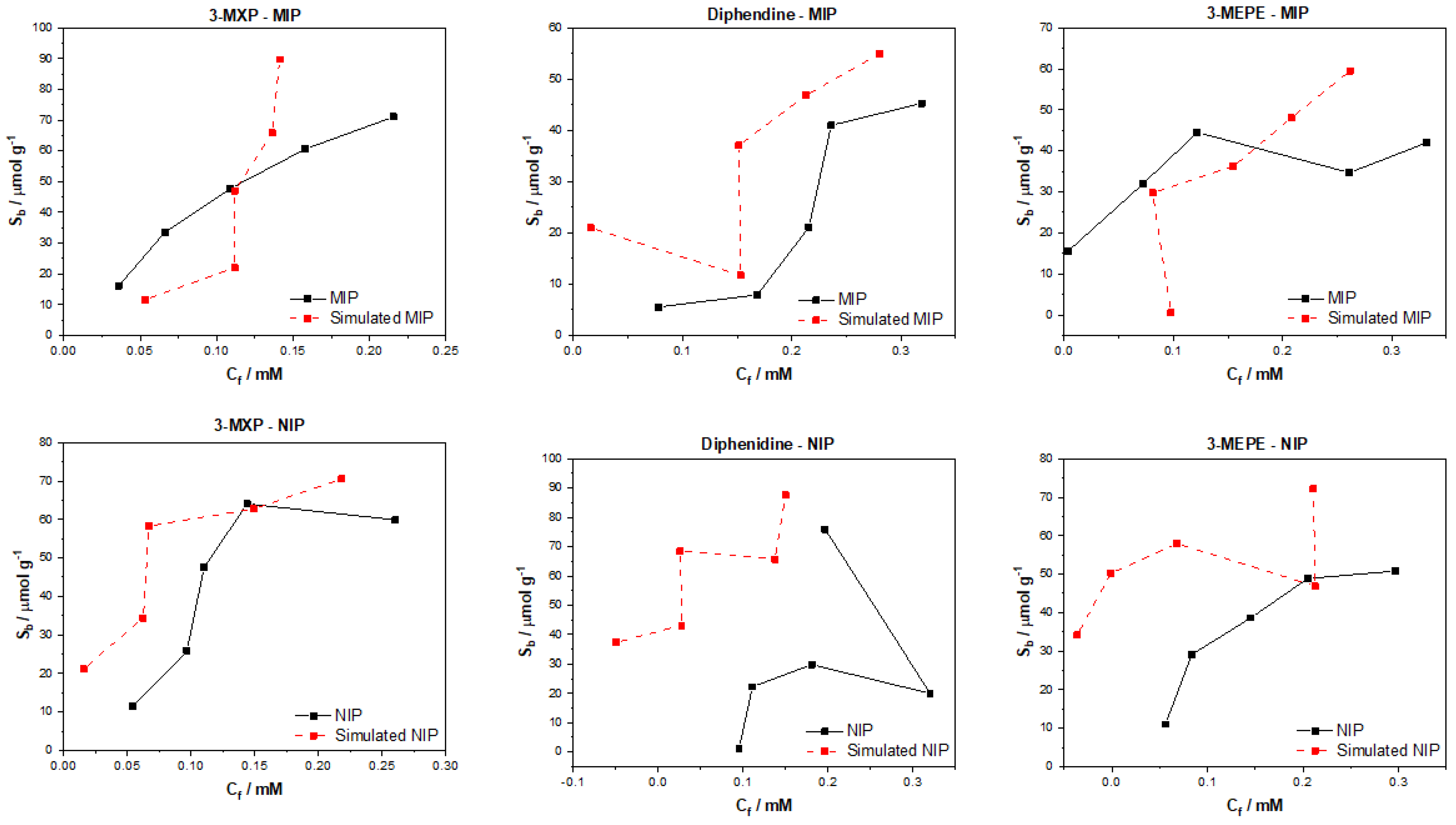
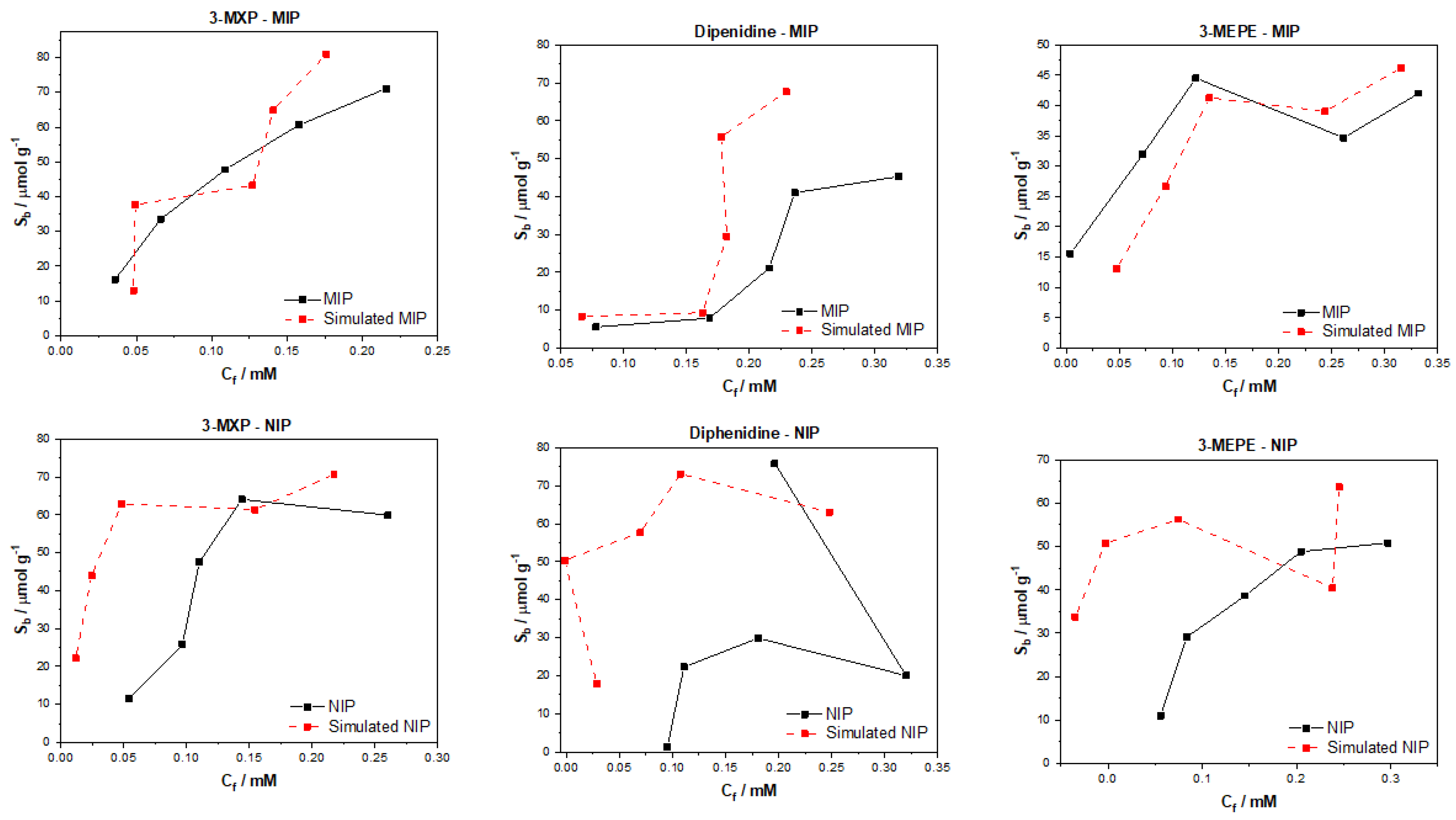
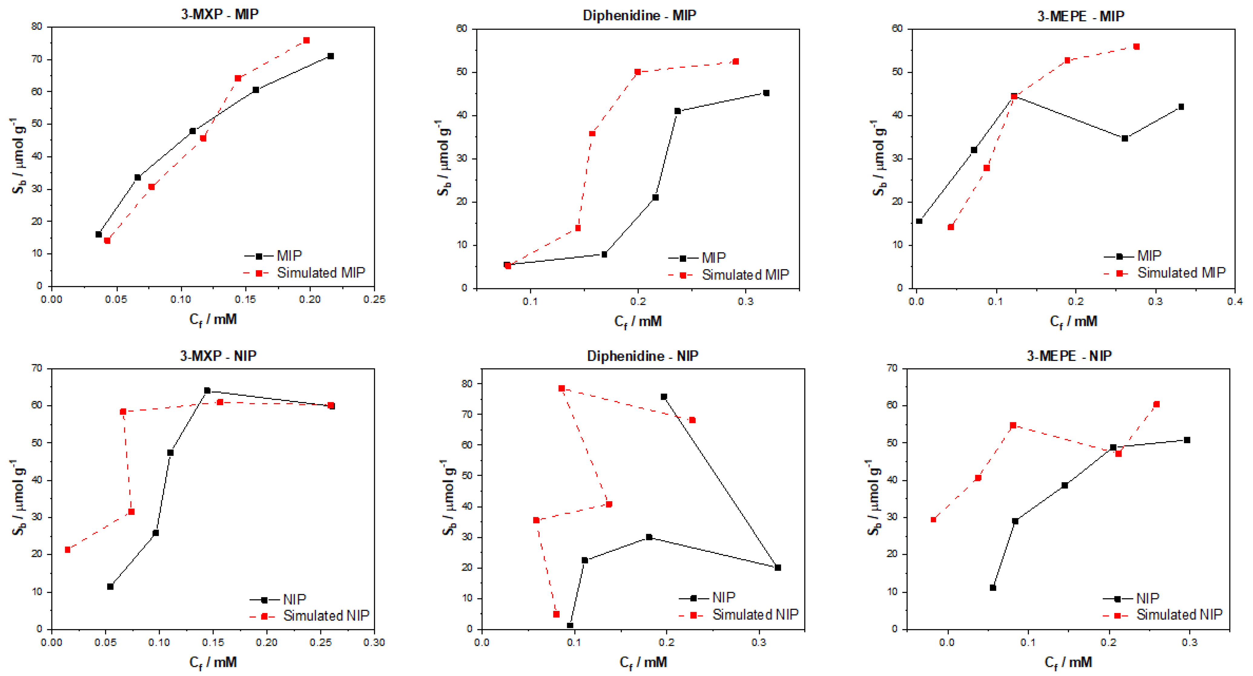
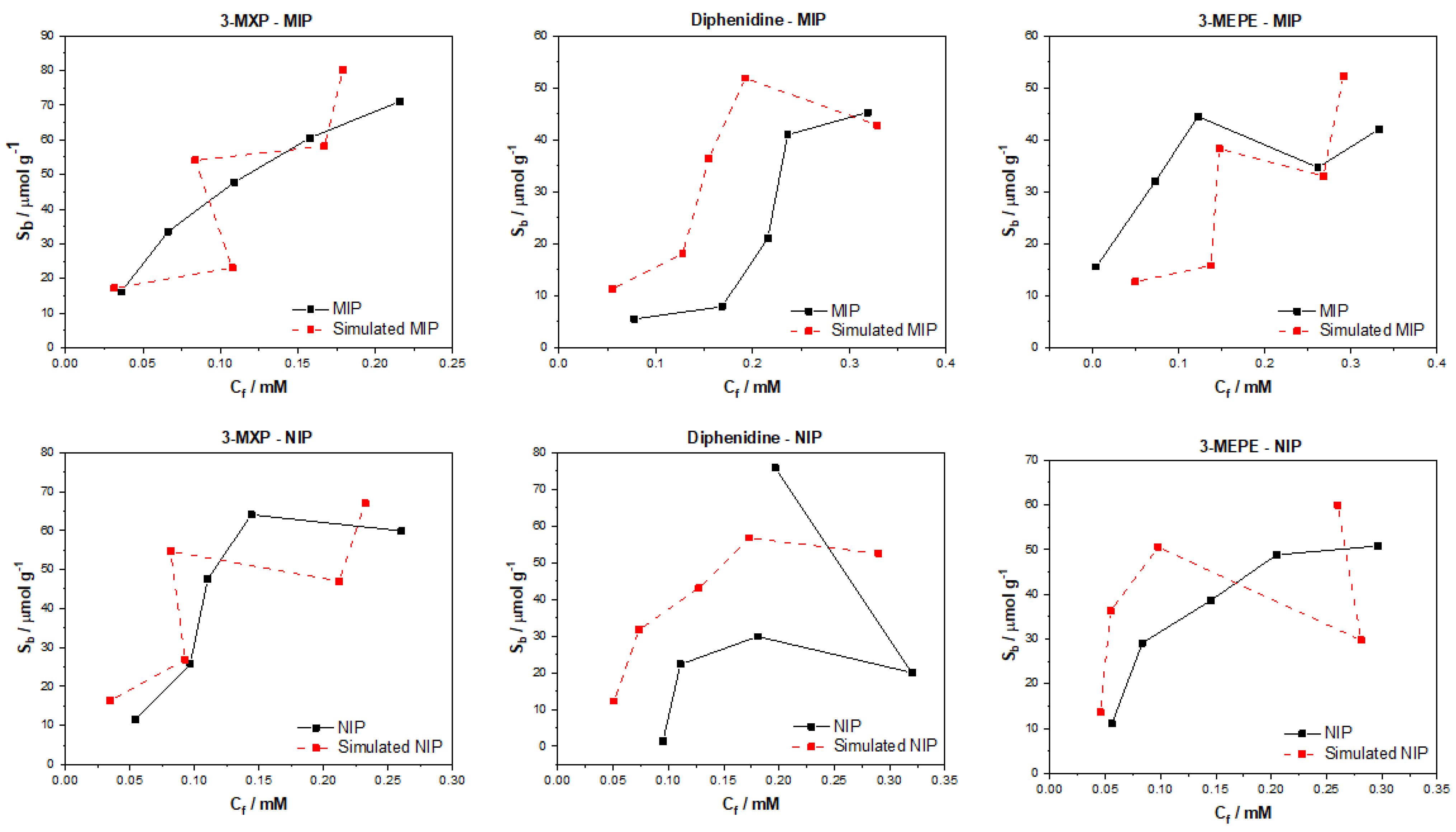
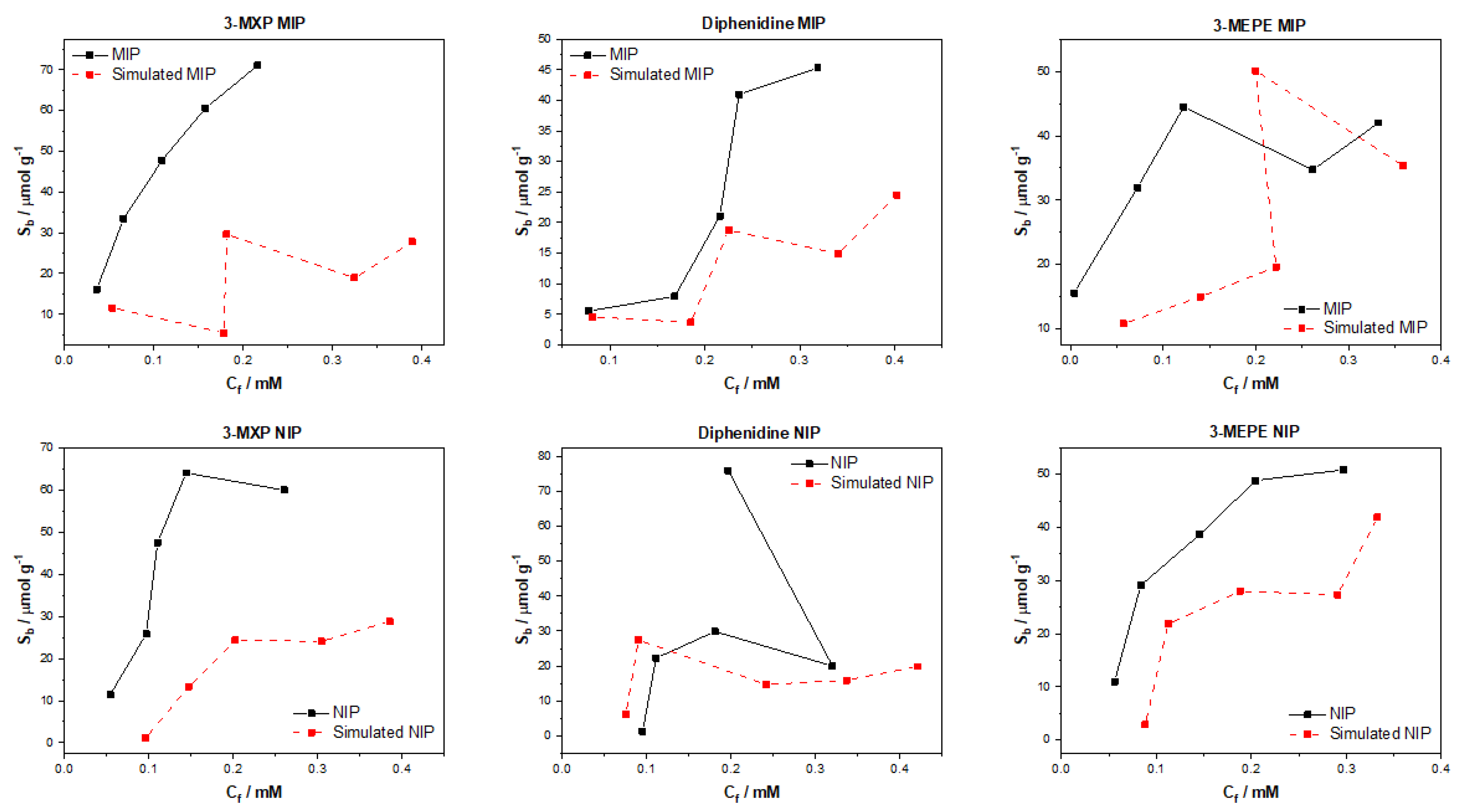
After testing the multiple algorithms for their potential in predicting MIP/NIP binding affinities, it can be concluded that there is great potential in these approaches for the simulation of MIP data. The most promising of these algorithms include the multitask regression and graph convolution models, with the simulated MIP data proving to be the most accurate representations of the experimental data discussed. The DAG, ChemCeption model and graph convolution with weave featurizer proved to have a harder time predicting the binding affinities of molecules, though DAG with modification could have the potential to predict the desired values better. The graph convolution and multitask regressor approaches could predict the trends in the experimental data, producing predicted values that were a fair representation of the testing data. The statistical analysis of all trained and tested models reveals that the models perform well when training but are weak when being tested. As previously mentioned, this is due to the limited dataset and the poor generalization of the models towards different molecules/data. Overall, though the models struggled with over or under predicting the Sb and Cf values, suggesting that additional chemical properties or a combination of algorithms might lead to a more rounded model for the prediction of these values and expansion of the datasets toward other molecules would be fruitful.
The data analyzed and simulated using these approaches were derived from MIP/NIPs synthesized by monolithic bulk polymerization. It should be mentioned that this approach produces relatively heterogeneous MIP/NIP samples with particle sizes and binding cavities randomly distributed throughout the material. The heterogeneous nature is followed into the generated binding isotherms with some of the experimental isotherms proving to have poor trends, and thus making them harder to learn via computational methods. In the future, a more homogenous MIP synthesis could be selected that would therefore lend itself to more homogenous MIP data that could prove easier for machine learning algorithms to learn and predict. Other factors such as MIP composition (monomers, crosslinkers, and porogens used) and MIP porosity could be factored into the models, building upon reliability and the precision of the approach.
The main take away from the research is that these algorithms can be applied to real world MIP/NIP binding data and can predict affinities that resemble experimental values. This opens up the possibility of utilizing this approach in real-world scenarios, with the manuscript highlighting that it is possible to computationally predict the binding of molecules to MIPs. This is the first instance of this to the authors’ knowledge and highlights the potential of machine learning algorithms in this field. The machine learning experiments presented have been conducted by scientists with limit knowledge in the field of machine learning, and have arguably produced results that warrant further investigation into the use of these algorithms in a deep context. If this knowledge was applied by users who have more experience with these models, then we believe that an algorithm and/or approach could easily be identified that could help predict the binding of molecules to specific MIP/NIP compositional chemistries. Thus, this basic research has the potential to open the door for rapid computational simulations of molecular binding affinities and could be used in the rapid analysis of MIPs, reducing material costs, analysis time, and chemical wastage.

Supplementary Materials

The following are available online at https://0-www-mdpi-com.brum.beds.ac.uk/article/10.3390/computation9100103/s1, Table S1: MIP training data. Table S2: NIP training data. Table S3: MIP testing data. Table S4: NIP testing data.

Author Contributions

Conceptualization, J.W.L. and H.D.; methodology, H.I. and J.W.L.; software, H.I. and M.K.K.; validation, J.W.L., K.E. and B.v.G.; formal analysis, M.C. and H.I.; investigation, H.I. and M.K.K.; resources, B.v.G.; data curation, J.W.L., H.I. and M.K.K.; writing—original draft preparation, J.W.L.; writing—review and editing, J.W.L., K.E. and M.C.; visualization, J.W.L.; supervision, H.D., K.E. and T.J.C.; project administration, T.J.C. and H.D.; funding acquisition, B.v.G., K.E. and H.D. All authors have read and agreed to the published version of the manuscript.

Funding

This research was funded by the province of Limburg (The Netherlands), grant “Limburg Meet”, in collaboration with SABER Print.

Data Availability Statement

The data is contained in the article, supplementary information and can also be requested from the corresponding author.

Acknowledgments

The authors are grateful to the DeepChem developer team, especially Bharath Ramsundar, Peter Eastman, Patrick Walters, Vijay Pande, Karl Leswing, and Zhenqin Wu, for establishing and maintaining the DeepChem infrastructure. The preliminary modelling conducted by Cyrille Sébert and Marc Astner was also greatly appreciated.

Conflicts of Interest

The authors declare no conflict of interest.

Appendix A. List of Optimized Hyperparameters for the Models

DAG model:
  • max_atoms = 50
  • n_atom_feat = 50, 75, 100
  • n_graph_feat = 30, 40, 50
  • n_outputs = 15, 30, 45
  • layer_sizes = [100], [150], [200]
  • layer_sizes_gather = [100], [150], [200]
  • mode = regression
  • n_classes = 2
RobustMultitaskRegressor:
  • Layer structure: three layers, 1000 nodes each
  • Learning rate: 0.0001
  • Dropout rate: 0.2
  • Featurizer: RDKit descriptors (size = 208)
GraphConvolution:
  • Hyperparameters changed from multitask to single task
  • Mode: regression
  • Number of tasks: 2
  • Parameters: Sb, Cf
  • Graph convolutional layers: ([256, 256]; [128, 128, 128]; [256, 256])
  • Dense layer size: 128
  • Dropout rate: (0.001; 0.00001; 0.01)
  • Number of atom features: (125; 125; 100)
GraphConvolution (weave featurizer):
  • n_weave = 1, 2
  • Mode: regression
  • Number of tasks: 2
  • Parameters: Sb, Cf
  • Graph convolutional layers: ([256, 256]; [128, 128, 128]; [256, 256])
  • Dense layer size: 128
  • Dropout rate: (0.001; 0.00001; 0.01)
  • Number of atom features: (125; 125; 100)
Chemception:
  • Hyperparameters changed from multitask to single task
  • Mode: regression
  • Augment: TRUE
  • Number of tasks: 2
  • Parameters: Sb, Cf
  • Number of base filters: (32; 32; 16)
  • Inception blocks: (A,B,C:3; A,B,C:3; A,B,C:9)

References

  1. Nayak, S.; Blumenfeld, N.R.; Laksanasopin, T.; Sia, S.K. Point-of-Care Diagnostics: Recent Developments in a Connected Age. Anal. Chem. 2017, 89, 102–123. [Google Scholar] [CrossRef] [PubMed] [Green Version]
  2. St John, A.; Price, C.P. Existing and Emerging Technologies for Point-of-Care Testing. Clin. Biochem. Rev. 2014, 35, 155–167. [Google Scholar] [PubMed]
  3. Kaur, H.; Shorie, M. Nanomaterial based aptasensors for clinical and environmental diagnostic applications. Nanoscale Adv. 2019, 1, 2123–2138. [Google Scholar] [CrossRef] [Green Version]
  4. Belbruno, J. Molecularly imprinted polymers. Chem. Rev. 2019, 119, 95–119. [Google Scholar] [CrossRef]
  5. Sharma, P.S.; Iskierko, Z.; Pietrzyk-Le, A.; D’Souza, F.; Kutner, W. Bioinspired intelligent molecularly imprinted polymers for chemosensing: A mini review. Electrochem. Commun. 2015, 50, 81–87. [Google Scholar] [CrossRef]
  6. Lowdon, J.W.; Diliën, H.; Singla, P.; Peeters, M.; Cleij, T.J.; van Grinsven, B.; Eersels, K. MIPs for Commercial Application in Low-cost Sensors and Assays—An Overview of the Current Status Quo. Sens. Actuators B Chem. 2020, 325, 128973. [Google Scholar] [CrossRef] [PubMed]
  7. Poma, A.; Guerreiro, A.; Whitcombe, M.J.; Piletska, E.V.; Turner, A.P.F.; Piletsky, S.A. Solid-phase synthesis of molecularly imprinted polymer nanoparticles with a reusable template—“Plastic Antibodies”. Adv. Funct. Mater. 2013, 23, 2821–2827. [Google Scholar] [CrossRef] [Green Version]
  8. Ambrosini, S.; Beyazit, S.; Haupt, K.; Bui, B.T.S. Solid-phase synthesis of molecularly imprinted nanoparticles for protein recognition. Chem. Commun. 2013, 49, 6746–6748. [Google Scholar] [CrossRef]
  9. Dorko, Z.; Nagy-Szakolczai, A.; Toth, B.; Horvai, G. The selectivity of polymers imprinted with amines. Molecules 2018, 23, 1298. [Google Scholar] [CrossRef] [Green Version]
  10. Alenazi, N.A.; Manthorpe, J.M.; Lai, E.P.C. Selectivity enhancement in molecularly imprinted polymers for binding of bisphenol A. Sensors 2016, 16, 1697. [Google Scholar] [CrossRef] [Green Version]
  11. Feng, F.; Lai, L.; Pei, J. Computational chemical synthesis analysis and pathway design. Front. Chem. 2018, 6, 199. [Google Scholar] [CrossRef] [Green Version]
  12. Cavasotto, C.N.; Aucar, M.G.; Adler, N.S. Computational chemistry in drug lead discovery and design. J. Quantum. Chem. 2019, 199, 25678. [Google Scholar] [CrossRef] [Green Version]
  13. Siddique, N.; Adeli, H. Nature inspired chemical reaction optimisation algorithms. Cogn. Comput. 2017, 9, 411–422. [Google Scholar] [CrossRef]
  14. Mamo, S.K.; Elie, M.; Baron, M.G.; Gonzalez-Rodriguez, J. Computationally desgined perrhenate ion imprinted polymers for selective trapping of rhenium ions. ACS Appl. Polym. Mater. 2020, 2, 3135–3147. [Google Scholar] [CrossRef]
  15. Woznica, M.; Sobiech, M.; Palka, N.; Lulinski, P. Monitoring the role of enantiomers in the surface modification and adsorption process of polymers imprinted by chrial molecules: Theory and practice. J. Mater. Sci. 2020, 55, 10626–10642. [Google Scholar] [CrossRef]
  16. Cowen, T.; Busato, M.; Karim, K.; Piletsky, S.A. Insilico synthesis of synthetic receptors: A polymerization algorithm. MacroMolecules 2016, 37, 2011–2016. [Google Scholar]
  17. Sobiech, M.; Zolek, T.; Lulinski, P.; Maciejewske, D. A computational exploration of imprinted polymer affinity based on coriconazole metabolites. Analyst 2014, 139, 1779–1788. [Google Scholar] [CrossRef] [PubMed]
  18. Maryasin, B.; Marquetand, P.; Maulide, N. Machine learning for organic synthesis: Are robots replacing chemists? Angew. Chem. 2018, 57, 6978–6980. [Google Scholar] [CrossRef]
  19. Balaraman, M.; Soundar, D. An artificial neural network analysis of porcine pancreas lipase catalyzed esterification of anthranilic acid with methanol. Proc. Biochem. 2005, 40, 3372–3376. [Google Scholar]
  20. Betiku, E.; Taiwo, A.E. Modeling and optimization of bioethanol production from breadfruit starch hydrolysate vis-à-vis response surface methodology and artificial neural network. Renew. Energy 2015, 74, 87–94. [Google Scholar] [CrossRef]
  21. Mater, A.C.; Coote, M.L. Deep learning in chemistry. J. Chem. Inf. Model. 2019, 59, 2545–2559. [Google Scholar] [CrossRef] [PubMed]
  22. Tkatchanko, A. Machine learning for chemical discovery. Nat. Commun. 2020, 11, 4125. [Google Scholar] [CrossRef] [PubMed]
  23. Mohapatra, S.; Dandapat, S.J.; Thatoi, H. Physicochemical characterization, modelling and optimization of ultrasono-assisted acid pretreatment of two pennisetum sp. Using Taguchi and artificial neural networking for enhanced delignification. J. Environ. Manag. 2017, 187, 537–549. [Google Scholar] [CrossRef]
  24. Ramsundar, B.; Kearnes, S.; Riley, P.; Webster, D.; Konerding, D.; Pande, V. Massively Multitask Networks for Drug Discovery. arXiv 2015, arXiv:1502.02072. [Google Scholar]
  25. Jiao, Z.; Hu, P.; Xu, H.; Wang, Q. Machine learning and Deep learning in chemical health and safety: A systematic review of techniques and applications. ACS Chem. Health Saf. 2020, 27, 316–334. [Google Scholar] [CrossRef]
  26. Sun, M.; Zhao, S.; Gilvary, C.; Elemento, O.; Zhou, J.; Wang, F. Graph convolutional networks for computational drug development and discovery. Brief. Bioinform. 2020, 21, 919–935. [Google Scholar] [CrossRef]
  27. Gonzalez-Diaz, H.; Perez-castillo, Y.; Podda, G.; Uriarte, E. Computational chemistry comparison of stable/nonstable protein mutants classification models based on 3D and topological indices. J. Comp. Chem. 2007, 28, 1990–1995. [Google Scholar] [CrossRef]
  28. Feinberd, E.N.; Joshi, E.; Pande, V.S.; Cheng, A.C. Improvement in ADMET prediction with multitask deep featurization. J. Med. Chem. 2020, 63, 8835–8848. [Google Scholar] [CrossRef]
  29. Jeon, W.; Kim, D. FP2VEC: A new molecular featurizer for learning molecular properties. Bioinfomatics 2019, 35, 4979–4985. [Google Scholar] [CrossRef]
  30. Toropov, A.A.; Toropova, A.P.; Benfenati, E.; Leszczynska, D.; Leszczynski, J. SMILES-based optimal descriptors: QSAR analysis of fullerene-based HIV-1 PR inhibitors by means of balance of correlations. J. Comp. Chem. 2009, 31, 381–392. [Google Scholar] [CrossRef]
  31. Baskin, I.I.; Winkler, D.; Tetko, I.V. A renaissance of neural networks in drug discovery. Expert Opin. Drug Discov. 2016, 11, 785–795. [Google Scholar] [CrossRef]
  32. Zhang, J.; Zhao, J.; Lin, H.; Tan, Y.; Cheng, J. High-speed chemical imaging by dense-net learning of femtosecond stimulated raman scattering. J. Phys. Chem. Lett. 2020, 11, 8573–8578. [Google Scholar] [CrossRef]
  33. Okuwaki, J.; Ito, M.; Mochizuki, Y. Development of educational scratch program for machine learning for students in chemistry course. J. Comp. Chem. 2020, 18, 126–128. [Google Scholar]
  34. Hutchinson, S.T.; Kobayashi, R. Solvent-specific featurization for predicting free energies of solvation through machine learning. J. Chem. Inf. Mod. 2019, 59, 1338–1346. [Google Scholar] [CrossRef] [PubMed]
  35. Janczura, M.; Lulinski, P.; Sobiech, M. Imprinting technology for effective sorbent fabrication: Current state-of-the-art and future prospects. Materials 2021, 14, 1850. [Google Scholar] [CrossRef] [PubMed]
  36. Suryana, S.; Rosandi, R.; Hasanah, A.N. An update on molecularly imprinted polymer design through a computational approach to produce molecular recognition material with enhanced analytical performance. Molecules 2021, 26, 1891. [Google Scholar] [CrossRef] [PubMed]
  37. Zapata, F.; Matey, J.M.; Montalvo, G.; Grcia-Ruiz, C. Chemical classification of new psychoative substances (NPS). Microchem. J. 2021, 163, 105877. [Google Scholar] [CrossRef]
  38. Castaing-Cordier, T.; Ldroue, V.; Besacier, F.; Bulete, A.; Jacquemin, D.; Giraudeau, P.; Farjon, J. High-field and benchtop NMR spectroscopy for the characterization of new psychoactive substances. Forensic Sci. Int. 2021, 321, 110718. [Google Scholar] [CrossRef] [PubMed]
  39. Valli, A.; Lonati, D.; Locatelli, C.A.; Buscagilia, E.; Tuccio, M.D.; Papa, P. Analytically diagnosed intoxication by 2-methoxphenidine and flubromazepam mimicking an ischemic cerebral disease. Clin. Toxicol. 2017, 55, 611–612. [Google Scholar] [CrossRef]
  40. Luethi, D.; Hoener, M.C.; Liechti, M.E. Effects of the new psychoactive substances diclofensine, diphenidine, and methoxphenidine on monoaminergic systems. Eur. J. Pharmacol. 2018, 819, 242–247. [Google Scholar] [CrossRef]
  41. Lowdon, J.W.; Eersels, E.; Rogosic, R.; Heidt, B.; Dilien, H.; Steen Redeker, E.; Peeters, M.; van Grinsven, B.; Cleij, T.J. Substrate displacement colorimetry fort he detection of diarylethylamines. Sens. Actuators B Chem. 2019, 282, 137–144. [Google Scholar] [CrossRef]
  42. Lowdon, J.W.; Alkirkit, S.M.O.; Mewis, R.E.; Fulton, D.; Banks, C.E.; Sutcliffe, O.B.; Peeters, M. Engineering molecularly imprinted polymers (MIPs) for the selective extraction and quantification of the novel psychoactive substance (NPS) methoxphenidine and its regioisomers. Analyst 2018, 9, 2002–2007. [Google Scholar] [CrossRef] [PubMed] [Green Version]
  43. Lusci, A.; Pollastri, G.; Baldi, P. Deep architectures and deep learning in chemoinformatics: The prediction of aqueous solubility for drug-like molecules. J. Chem. Inf. Model. 2013, 53, 1565–1575. [Google Scholar] [CrossRef] [PubMed] [Green Version]
  44. Son, J.; Kim, D. Development of a graph convolutional neural network model for efficient prediction of protein-ligand binding affinities. PLoS ONE 2021, 16, e0249404. [Google Scholar] [CrossRef] [PubMed]
  45. Tan, Z.; Li, Y.; Shi, W.; Yang, S. A multitask approach to learn molecular properties. J. Chem. Inf. Model. 2021, 61, 3824–3834. [Google Scholar] [CrossRef] [PubMed]
  46. Kearnes, S.; McCloskey, K.; Berndl, M.; Pande, V.; Riley, P. Molecular graph convolutions: Moving beyond fingerprints. J. Comp. Mol. Des. 2016, 30, 595–608. [Google Scholar] [CrossRef] [PubMed] [Green Version]
  47. Coley, C.W.; Green, W.H.; Jensen, K.F. RDChiral: An RDKit wrapper for handling stereochemistry in retrosynthetic template extraction and application. J. Chem. Inf. Model. 2019, 59, 2529–2537. [Google Scholar] [CrossRef]
  48. Yoo, Y. Hyperparameter optimization of deep neural network using univariate dynamic encoding algorithm for searches. Knowl. Based Syst. 2019, 178, 74–83. [Google Scholar] [CrossRef]
  49. D’souza, R.N.; Huang, P.; Yeh, F. Structural analysis and optimization of convolutional neural networks with a small sample size. Sci. Rep. 2020, 10, 834. [Google Scholar] [CrossRef]
Figure 1. Examples of how a molecule (2-methoxphenidine) can be converted into a directed acyclic graph (DAG), and then how the sum of different root versions of the DAG are used for a prediction.
Computation 09 00103 g001
Figure 2. The concept behind the graph convolution model, stemming from the conversion of a model compound (2-methoxphenidine) into nodes that are ready for convolution and graphing.
Computation 09 00103 g002
Figure 3. The concept behind the multitask regressor algorithm, simultaneously predicting values based off different chemical properties and then merging these values to generate an overall numerical prediction.
Computation 09 00103 g003
Figure 4. The concept behind the ChemCeption methodology of generating a neural network that relates the 2D structure of a molecule to a trained chemical property.
Computation 09 00103 g004
Figure 5. DAG simulated and experimental binding isotherms for MIP and NIP in regard to the binding of 3-MXP, diphenidine, and 3-MEPE.
Computation 09 00103 g005
Figure 6. Multitask regressor with the RdKit featurizer simulated and experimental binding isotherms for MIP and NIP in regard to the binding of 3-MXP, diphenidine, and 3-MEPE.
Computation 09 00103 g006
Figure 7. Graph convolution simulated and experimental binding isotherms for MIP and NIP in regard to the binding of 3-MXP, diphenidine, and 3-MEPE.
Computation 09 00103 g007
Figure 8. Graph convolution with a weave featurizer simulated and experimental binding isotherms for MIP and NIP in regard to the binding of 3-MXP, diphenidine, and 3-MEPE.
Computation 09 00103 g008
Figure 9. ChemCeption model with SMILEStoImage featurizer simulated and experimental binding isotherms for MIP and NIP in regard to the binding of 3-MXP, diphenidine, and 3-MEPE.
Computation 09 00103 g009
Table 1. Analysis of the error and correlation of the trained datasets at a given Ci value.
SbCf
CiR2Pearson R2MAE ScoreR2Pearson R2MAE Score
MIP0.10.99890.99990.4520.99990.99990.153
0.20.99990.99990.00030.99980.99980.0005
0.30.99990.99990.0550.99990.99992.683
0.40.99990.99990.0010.99990.99990.000006
0.50.99990.99990.0010.99990.99990.00001
NIP0.10.99990.99990.1630.99990.99990.00003
0.20.99990.99990.00040.99990.99990.000007
0.30.99990.99990.0060.99990.99990.000003
0.40.99990.99990.0010.99990.99990.000006
0.50.99990.99990.0020.99990.99990.000001
Table 2. Analysis of the error and correlation of the test datasets at a given Ci value.
SbCf
CiR2Pearson R2MAE ScoreR2Pearson R2MAE Score
MIP0.10.33420.450412.420.97760.989713.71
0.20.61020.75696.8090.84960.90270.019
0.30.77200.84096.6530.83210.83230.025
0.40.51690.956812.560.93780.96890.023
0.50.48130.954912.440.78320.83140.051
NIP0.10.01640.098113.530.13040.12810.039
0.20.27690.731314.720.63550.68530.022
0.30.58850.803516.590.71380.71930.029
0.40.31570.422616.200.45550.48630.066
0.50.56710.913413.670.92470.93810.030
Table 3. Analysis of the error and correlation of the trained datasets at a given Ci value for the multitask regressor model.
SbCf
CiR2Pearson R2MAE ScoreR2Pearson R2MAE Score
MIP0.10.91570.94983.9220.97010.978717.42
0.20.64790.67915.2580.39210.48430.191
0.30.72150.83055.9580.49440.79810.150
0.40.81430.82897.3920.69230.77690.209
0.50.84500.84508.5080.62720.81220.172
NIP0.10.95210.97122.3440.01100.06890.188
0.20.93410.93754.0730.82760.44450.236
0.30.92110.96574.9730.21760.69630.193
0.40.92780.95034.3160.64540.75150.196
0.50.85570.86177.8080.11170.87590.168
Table 4. Analysis of the error and correlation of the test datasets at a given Ci value for the multitask regressor model.
SbCf
CiR2Pearson R2MAE ScoreR2Pearson R2MAE Score
MIP0.10.52310.550110.400.89330.980522.25
0.20.71570.87596.2260.12070.24650.215
0.30.67340.82429.2280.46420.64490.183
0.40.76780.89928.1990.41640.90230.239
0.50.22030.830218.300.81200.95650.191
NIP0.10.44810.537411.460.31880.77900.1997
0.20.57290.933011.200.28710.70030.2561
0.30.69880.90937.5390.09130.04620.225
0.40.01570.435914.850.28730.81300.222
0.50.65360.878412.920.25330.84270.221
Table 5. Analysis of the error and correlation of the trained datasets at a given Ci value for the graph convolution model.
SbCf
CiR2Pearson R2MAE ScoreR2Pearson R2MAE Score
MIP0.10.99990.99990.0190.75220.913329.92
0.20.99990.99990.0120.95790.98300.011
0.30.99990.99990.0550.98970.99290.009
0.40.99960.99980.2940.99040.99120.010
0.50.99650.99881.0470.99300.99780.011
NIP0.10.99990.99990.0400.94540.95730.011
0.20.99990.99990.1070.99420.99450.005
0.30.99990.99990.0960.99170.99230.009
0.40.99960.99980.2880.99420.99420.011
0.50.99860.99940.7080.99880.99890.004
Table 6. Analysis of the error and correlation of the test datasets at a given Ci value for the graph convolution model.
SbCf
CiR2Pearson R2MAE ScoreR2Pearson R2MAE Score
MIP0.10.26710.52837.6340.33710.682913.43
0.20.54780.86457.4190.22480.62300.240
0.30.68680.73858.6850.24460.45950.308
0.40.15130.665513.970.15440.02310.301
0.50.45710.728220.200.00650.00620.345
NIP0.10.47240.60988.8180.57820.63950.251
0.20.42510.94046.4850.05630.05310.309
0.30.63280.94088.8240.00580.00130.442
0.40.34220.370515.880.44950.75240.409
0.50.58750.828913.050.11830.23550.348
Table 7. Analysis of the error and correlation of the trained datasets at a given Ci value for the graph convolution model with weave featurizer.
SbCb
CiR2Pearson R2MAE ScoreR2Pearson R2MAE Score
MIP0.10.96760.98202.7420.40110.74597.191
0.20.94170.96102.4310.77650.86780.261
0.30.97070.98922.7540.18960.11420.147
0.40.90750.94885.6450.34420.46410.366
0.50.039250.157128.560.17520.54570.117
NIP0.10.10660.972713.180.02040.08880.218
0.20.96870.98133.3620.03740.03710.109
0.30.94930.98124.9300.16970.13520.362
0.40.37150.855316.880.02340.16100.7454
0.50.77660.883813.140.42460.80270.327
Table 8. Analysis of the error and correlation of the test datasets at a given Ci value for the graph convolution model with weave featurizer.
SbCf
CiR2Pearson R2MAE ScoreR2Pearson R2MAE Score
MIP0.10.61820.63579.7250.87610.95913.591
0.20.61140.91096.8520.62490.70890.163
0.30.51320.63339.8450.33560.39520.162
0.40.53710.969111.700.83010.92610.628
0.50.054790.398915.280.78280.95620.049
NIP0.10.19620.52916.6800.20530.81940.338
0.20.12840.857914.090.18760.62240.073
0.30.32830.921912.050.72590.88820.501
0.40.56660.157525.040.47270.75070.755
0.50.57740.607110.100.63230.90360.450
Table 9. Analysis of the error and correlation of the trained datasets at a given Ci value for the graph ChemCeption model with SMILESToImage featurizer.
SbCf
CiR2Pearson R2MAE ScoreR2Pearson R2MAE Score
MIP0.10.99990.99990.016380.99990.99990.075
0.20.99970.99990.60110.99990.99990.000007
0.30.99990.99990.46710.99990.99990.0000004
0.40.99970.99990.067480.99990.99990.000001
0.50.99990.99990.0990.99990.99990.0000007
NIP0.10.99990.99990.012710.99990.99990.0000004
0.20.99990.99990.004750.99990.99990.0000008
0.30.99990.99990.013150.99990.99990.0000006
0.40.99990.99990.20950.99990.99990.0000004
0.50.99990.99990.12070.99990.99990.0000003
Table 10. Analysis of the error and correlation of the test datasets at a given Ci value for the ChemCeption model with SMILESToImage featurizer.
SbCf
CiR2Pearson R2MAE ScoreR2Pearson R2MAE Score
MIP0.10.44430.06724.6020.03480.288868.29
0.20.32780.261111.660.09300.12380.042
0.30.25570.585513.650.32380.38160.045
0.40.09970.0001722.189530.30020.30520.070
0.50.25290.573116.450.34850.30570.096
NIP0.10.11780.119954.92510.03500.15840.025
0.20.10830.38919.04140.57050.73380.027
0.30.0084530.0000128419.47870.64290.67400.030
0.40.011880.0393826.950.47900.49420.059
0.50.076710.0125329.33620.64630.68720.054
Publisher’s Note: MDPI stays neutral with regard to jurisdictional claims in published maps and institutional affiliations.

