
Exact Boolean Abstraction of Linear Equation Systems


1
CRIStAL—Centre de Recherche en Informatique, Signal et Automatique de Lille—UMR 9189, Université de Lille—Campus Scientifique, 59655 Villeneuve-d’Ascq, France
2
Faculte des Sciences et Technologies, University of Lille, 59650 Villeneuve-d’Ascq, France
3
Inria, Université de Lille, 59000 Lille, France
*
Author to whom correspondence should be addressed.
†
These authors contributed equally to this work.
Computation 2021, 9(11), 113; https://0-doi-org.brum.beds.ac.uk/10.3390/computation9110113
Submission received: 31 July 2021
/
Revised: 11 October 2021
/
Accepted: 12 October 2021
/
Published: 21 October 2021
(This article belongs to the Special Issue Formal Method for Biological Systems Modelling)
Abstract
:We study the problem of how to compute the boolean abstraction of the solution set of a linear equation system over the positive reals. We call a linear equation system ϕ exact for the boolean abstraction if the abstract interpretation of ϕ over the structure of booleans is equal to the boolean abstraction of the solution set of ϕ over the positive reals. Abstract interpretation over the booleans is thus complete for the boolean abstraction when restricted to exact linear equation systems, while it is not complete more generally. We present a new rewriting algorithm that makes linear equation systems exact for the boolean abstraction while preserving the solutions over the positive reals. The rewriting algorithm is based on the elementary modes of the linear equation system. The computation of the elementary modes may require exponential time in the worst case, but is often feasible in practice with freely available tools. For exact linear equation systems, we can compute the boolean abstraction by finite domain constraint programming. This yields a solution of the initial problem that is often feasible in practice. Our exact rewriting algorithm has two further applications. Firstly, it can be used to compute the sign abstraction of linear equation systems over the reals, as needed for analyzing function programs with linear arithmetics. Secondly, it can be applied to compute the difference abstraction of a linear equation system as used in change prediction algorithms for flux networks in systems biology.
1. Introduction
We develop approaches to remedy the incompleteness of abstract interpretation [1] of linear equation systems over the reals, in the algebra of booleans and the structure of signs . These abstractions have various applications: in systems biology, the boolean abstraction underlies abstractions of chemical reactions networks into Boolean networks [2,3]. In program analysis, the sign abstraction can be applied to functional programs with arithmetics for analyzing the signs of the possible values of floating-point variables [4,5].
The soundness of abstract interpretations of first-order logic formulas without negation was shown by John [6,7,8,9]. It applies to the interpretation in any concrete structure S, as long as it is connected by a homomorphism to the abstract structure . The concrete interpretation of a first-order formula is the set of concrete solutions , and its abstract interpretation is the set of its abstract solutions . John’s soundness theorem (see Theorem 1 below) states that the set of abstract solutions of overapproximates the abstraction by h of the set of concrete solutions:
When choosing the operators in , the class of negation-free first-order formulas with operators in extends on the classes of linear and polynomial equation systems. In this article, we consider the boolean abstraction which is the unique homomorphism , and the sign abstraction which is the unique homomorphism with respect to the operators in . The boolean abstraction maps any strictly positive real to 1 and 0 to 0. The sign abstraction extends on the boolean abstraction while mapping all strictly negative reals to . We note that the structure of signs is not an algebra since the sum of a positive and a negative number may have any sign.
1.1. Problematics
A natural question is whether abstract interpretation is complete [10] for the abstraction of formulas induced by a homomorphisms , i.e, whether for all negation-free first-order formulas with the same operators:
We call a formula h-exact if it satisfies this property. A counter example against the completeness of abstraction interpretation for the boolean and the sign abstraction is the linear equation equal to . Here, we write for the equality symbol inside the logic, to point out its difference from equality in the language of mathematics. Formula is neither -exact nor -exact. This can be seen as follows. Over the reals is equivalent to , so that all assignments that are abstractions of concrete solutions of must satisfy . When interpreted abstractly over or , however, admits the abstract solution which is not the abstraction of any concrete solution since .
To deal with the incompleteness of abstract interpretation, we propose to study the following two questions for homomorphism where h is either the boolean abstraction or the sign abstraction .
Exact Rewriting Can we rewrite linear equation systems to h-exact formulas?
Computing Abstractions Can we can compute the abstraction exactly for a given system of homogeneous linear equations ?
Geometrically speaking, the concrete solution sets and of homogeneous linear equation systems are polytopes—i.e., finite intersections of half-spaces in . The problem of computing boolean abstractions or sign abstraction is thus to compute the abstraction of a polytope given by a linear equation system.
For any h-exact formula , the computation of abstractions is equivalent to the computation of . Since the abstract structure is finite for the boolean and sign abstraction, we can compute the set of abstract solutions in at most exponential time by a naive generate and test algorithm. Finite domain constraint programming [11] can by used to avoid the naive generation of all variable assignments to in many practical cases. Therefore, any algorithm for exact rewriting induces an algorithm for computing abstractions that may be feasible in practice.
1.2. Contributions
Our main result is the first algorithm for exact rewriting that applies to linear equation systems for the Boolean abstraction. Based on this algorithm, we present a novel algorithm for computing the sign abstraction of linear equation systems.
Exact Rewriting for the Boolean Abstraction. In the first step, we study exact rewriting of (homogeneous) linear equation systems for boolean abstraction. The counter example , for instance, can be rewritten to -exact formula . The idea is to take the system of all linear consequences over of the linear equation system. There may be infinitely many such consequences, but all of them are linear combinations of the extreme rays of the cone . Up to normalization, there are only finitely many extreme rays, which are known as the elementary modes of the linear equation system [12,13,14,15]. These can be computed by libraries from computational geometry [16] in at most exponential time. Nevertheless, the computation is often well-behaved in practice.
Based on the elementary modes (Folklore Theorem 2), we can rewrite any (homogeneous) linear equation system into quasi-positive and strongly-triangular linear equation system that is equivalent over (Corollary 1), that can be computed in at most exponential time. As we prove, such systems are always -exact (Theorem 3). Hence, any system of linear equations can be converted in at most exponential time to some -equivalent -exact formula.
Note that -exact formulas may still not be -exact. A counter example is the strongly-triangular quasi-positive linear system . It is not -exact, since it entails over but still has the abstract solution over which maps x and y to distinct signs. Indeed, we don’t have any idea of how to do exact rewriting for the sign abstraction. The problem is that positivity is essential for our approach, and since the addition of positive and negative numbers may have any sign, fails to be an algebra, making the analogous argument as in the proof of -exactness fail.
Extension to -Mixed Systems. In the second step, we introduce -mixed systems, which by Theorem 4 generalize on systems of 1. linear equations, 2. positive polynomial equations , and 3. positive polynomial inequations , where p is a positive polynomial without constant term. We then show our main result:
Theorem 5 (Main). Any -mixed systems can be converted to a -exact formula by converting its linear subsystem to an -exact formula.
The correctness of the algorithm for -mixed systems relies on the notion of -invariant formulas that we introduce. The class of -invariant formulas subsume systems of positive polynomial equations and inequations , where p is a positive polynomials without constant terms.
Computing Sign Abstractions. In the third step, we present an algorithm for computing the sign abstraction of (homogeneous) systems of linear equations based on exact rewriting for the boolean abstraction (Theorem 6). For this, we decompose the sign abstraction into the boolean abstraction based on a function that is definable in first-order logic. This function decomposes real numbers into their positive part x and negative part y. At least one of these two parts must be zero, which can be expressed by the polynomial equation . The positivity of x can be expressed by and the positivity of y in analogy. In this way, we can reduce the problem of computing to the problem of computing for some existentially quantified -mixed system that we can make -exact based on our main Theorem 5.
Application to Program Analysis. We show how to apply the computation of the sign abstraction of linear equation systems to improve the analysis of functional programs with arithmetics. For finding program errors there it can be useful to know about the possible signs of the values of program variables. We elaborate an example in the final Section 10.
Implementation. We implemented the -exact rewriting algorithm for -mixed systems from the main Theorem 5 in Python. For this we used a library from computational geometry [16] for computing elementary modes. We also used finite domain constraint programming with Minizinc [17] for computing the set of boolean solutions over logical formulas. Some successful experiments are mentioned in the related work subsection below. We did not yet implemented the algorithm for computing sign abstractions, nor its application to program analysis though.
1.3. Related Work
We start with related work by the authors, and then move to related work by others.
Change Prediction of Reaction Networks. Our main Theorem 5 was recently applied to the change prediction of reaction networks in systems biology [6]. Indeed, the development of the present article was originally motivated by this application. The problem there is to compute the difference abstraction of linear equation systems, expressing the steady state semantics of chemical reaction networks. Two difference abstractions were considered, and a refinement thereof . In analogy to the approach adopted for computing sign abstractions (step three above), the algorithmic approach presented there is to decompose the difference abstractions and into the boolean abstraction and functions that are definable in first-order logic. The elaboration of this approach, however, is quite different for reflecting the nature of the difference abstractions.
Experimentation. We tested our implementation of the exact rewriting algorithm for the boolean abstraction successfully for computing difference abstractions in the application of change prediction in systems biology. The experimental results are presented in [6] are generally encouraging. They show that -exact rewriting based on elementary modes in combination with finite domain constraint programming may indeed avoid naive generate and test in many practical examples. In some of these examples, however, the overall computation time still took some hours.
Abstracting Reaction Networks to Boolean Networks. Independently, the authors proposed an abstraction of chemical reaction networks to boolean networks in [18], whose precision can be improved by using the -exact rewriting of -mixed equation systems.
Alternative Algorithm for Computing Sign Abstractions. An alternative algorithm for computing the sign abstraction of linear equation systems (and thus also the boolean abstraction) can be obtained by John’s overapproximation Theorem 1. It shows that it is sufficient to generate the finitely many abstract solutions in , and then to check for each of them whether there exists a concrete solution such that . To perform this latter test, note that is equivalent to the strict inequation and by the equation . Similarly, can be defined by the strict inequation . Whether there exists a concrete solution such is thus equivalent to the satisfiability of over , where is the set of free variables of . The satisfiability of systems of strict linear inequations and homogeneous linear equations without constant terms over are known to be decidable since at least 1926 [19]. But still, one has to generate the set of all abstract solutions . The new algorithm presented above avoids generating this set.
Abstract Program Interpretation over Numerical Domains. In abstract interpretation [20], nonrelational domains permit to approximate the set of values of program variables while ignoring the relationship to the values of others. Well-known nonrelational numerical domains include the interval domain [21] describing invariants of the form with reals and the constant propagation domain for invariants of the form [22].
Abstract interpretation of relational domains may yield better approximations that with nonrelational domains, since relationships between the values of different variables can be taken into account. Well-known relational numerical domains include the polyhedral domain [4]. A polyhedron is the solution set of systems of inhomogeneous linear inequations of the form . Alternatively, the linear equality domain [23] was considered. These are defined by system of inhomogeneous linear equations .
In the present paper, we study the problem of computing the sign abstraction of polytopes represented by homogeneous linear equation systems. The polytopes can be obtained by existing methods for the abstract program interpretation over the polyhedral domain. One weakness of our approach is that we study the homogeneous case only, so that we can only abstract polytope and not more general polyhedrons.
1.4. Outline
In Section 2, we recall preliminaries on homomorphisms between -structures. In Section 3, the first-order logic is recalled. John’s theorem and its relation to the soundness and completeness of abstract interpretation in the classical framework are discussed in Section 4. We discuss how to make linear equation system quasipositive and strongly triangular based on elementary modes in Section 5. These properties can be used to prove -exactness as we show in Section 6, and thus to obtain an -exact rewriting of linear equation systems. We introduce the notion of -invariance in Section 7 and apply it in Section 8 to lift the -exact rewriting algorithm from linear to -mixed systems. This allows us to define the sign abstraction of linear equation systems on Section 9. We finally apply this result in Section 10 to the sign analysis of functional programs with arithmetic.
2. Homomorphisms on -Structures
We need some basic notation from set theory and standard notion of universal algebra such as -algebras, -structures, and homomorphism.
For any set A and , the set of n-tuples of elements in A is denoted by . For finite sets A the number of elements of A is denoted by . Furthermore, for any function we define the function such that for all .
2.1. -Algebras
We next recall the notion of -algebras. Let be a ranked signature. We call the elements of are called n-ary function symbols, even though we may also use them as -ary relation symbols later on when moving to -structures. The elements in are called the constants of .
Definition 1.
A-algebra consists of a set and an interpretation such that for all , and for all .
Let be the set of booleans, the set of natural numbers including 0, the set of integers, the set of real numbers, and the set of positive real numbers including 0. Note that and . Let the addition on the reals be the binary function and the multiplication the binary function . Let the addition on the positive real numbers be equal to the restriction and the multiplication be the restriction .
Let be the set of boolean operators where + and * are binary function symbols and 0 and 1 constants. Note that constant 0 is freely overloaded with the boolean 0 and the constant 1 with the boolean 1.
Example 1.
The set of positive reals can be turned into a -algebra, in which the functions symbols are interpreted as binary functions and . The constants are interpreted by themselves and .
Example 2.
The set of Booleans equally defines a -algebra. There, the function symbols are interpreted as a disjunction and conjunction on Booleans. The constants are interpreted by themselves and .
2.2. -Structures
We next recall the usual generalization of -algebras to -structures. The objective is to generalize from functions to relations. For this, we consider n-ary function symbols as -ary relation symbols.
Definition 2.
A-structure consists of a set and an interpretation such that for all and for all .
Clearly, any -algebra is also a -structure. Note also that symbols in are interpreted as monadic relations, i.e., as subsets of the domain, in contrast to constants in C that are interpreted as elements of the domain.
We denote the subtraction on the reals by the binary function and the division on the reals by the ternary relation . Note that division by zero is undefined. Note also that subtraction on would yield only a partial function.
Let be the arithmetic signature, where 0 and 1 are constants, and all other operators are binary function symbols. Again, we freely overlead to constant 0 with real number 0 and the constant 1 with the real number 1.
Example 3.
The set of reals can be turned into a -structure, with the interpretation of the binary functions symbols as the ternary relations , , , . The constants are interpreted by themselves and . Note that is a partial but not a total function, since division by 0 is not defined. So we must see as a ternary relation, so that is not a -algebra. It still is a -algebra though.
Example 4.
The set of signs can be turned into a -structure with the interpretation , , and, given in Figure 1. The constants are interpreted by themselves and . Note that all contains , and meaning that the sum of a strictly negative and a strictly positive real has a sign in , so it may either be strictly positive, strictly negative, or zero. So is a -structure and even when restricting the signature to it remains a -structure that is not a -algebra.
2.3. Homomorphisms
We recall the standard notion of homomorphism for -structures which can also be applied to -algebras.
Definition 3.
A homomorphism between two Σ-structures S and Δ is a function such that for , , , and :
- 1
- , and
- 2
- if then .
We can convert any -ary relation to a n-ary set valued functions. In this way, any n-function is converted to a n-ary set valued n-functions. In other words, functions of type are converted to functions of type where . In set-valued notation, the second condition on homomorphism can then be rewritten equivalently as . A homomorphism for -algebras thus satisfies and for all function symbols and it satisfies
The boolean abstraction is the function with and if .
Lemma 1.
The boolean abstraction is a homomorphism between -algebras.
Proof.
For all we have:
Hence, and . Finally, for both constants we have that . □
The sign abstraction is the function with , for all strictly negative reals and for all strictly positive reals .
Lemma 2.
The sign abstraction h𝕊 is a homomorphism between -structures.
Proof.
Let . For the multiplication we have and thus . For the addition, we have to distinguish cases. If r and have the same sign, so has the same sign, so that we have . If and or vice versa then we have so that . The treatment of and is similar. For the constants, we have and . □
3. First-Order Logic
We recall the syntax and semantics of first-order logic with equality. For this, we fix a countably infinite set of variables that will be ranged over by .
3.1. Expressions
Given a ranked signature with constants and function symbols , the set of -expressions contains all terms that can be constructed from constants and variables by using function symbols:
| ::= | where , , , |
Let be the set of all variables that occur in e. Given a subset let be the subset of expression with .
The semantics of -expressions is defined in Figure 2. For any -structure S and variable assignment , any expression denotes a set of values . This set is defined recursively by set-valued interpretation of the operators of the expressions in the structure S. If S is a -algebra, then the result will always be a singleton.
3.2. Logic Formulas
The set of first-order formulas is the set of terms constructed with the usual first-order connectives from equations with symbols in and variables in :
| ::= | where and |
A -formula is a term, which either is a -equation with variables in , an existentially quantified formula , a conjunction , or a negation . A system of -equations is a conjunction of equations where .
The set of free variables contains all those variables of that occur outside the scope of any existential quantifier in . Given a subset we write for the subset of formulas such that .
First-order formulas can be defined for providing the missing logical operators. Firstly, we can define disjunctions and implications , and secondly, universally quantified formulas . Note that these formulas are not negation-free (and thus John’s theorem cannot be applied to them). Third, we define the valid formula . Fourth, we write instead of . In the case the conjunction is . Fifth, for any vector of variables we will write instead of .
For any , the semantics of first-order formulas for a -structure S and a variable assignment is the truth value defined in Figure 3.
Note that the equality symbol is interpreted as nondisjointness, i.e., an equation is true if and only if . In the case of -algebras, the equality symbol is indeed interpreted as equality of singletons. In the case of more general -structures, though, it is not interpreted as set equality.
The set of solutions with domain V of a formula over a -algebra S is:
If we omit the index V, i.e., .
Two formulas are called S-equivalent if they have the same solution sets over S on , that is . Note that is equivalent to and also to , i.e., to .
3.3. Examples
Since we can define the boolean abstraction by a formula in over with two variables :
Since we can define the sign abstraction by a formula in over with two variables :
where:
These definitions illustrate that both abstraction are closely related to strict inequations and . The boolean abstraction is concerned with strict positivity , while the sign abstraction is also concerned with strict negativity .
3.4. Semantic Properties of Free and Bound Variables
We need the following two standard lemmas on the role of free and bound variables for the solution sets of logic formulas. For any subset of variable assignments R of type and any disjoint sets of variables we define .
Lemma 3
(Cylindrification). If then .
Proof.
We can show that for all expressions with disjoint to V and any variable assignment by induction on the structure of expressions. From this, we can prove for all formulas such that is disjoint from V and that by induction on the structure of -formulas. This implies the lemma. □
The projection of a function is its restriction . The projection of a set F of functions is .
Lemma 4
(Quantification is projection). .
Proof.
This is follows from the semantics of existential quantified formulas as follows:
□
4. Abstract Interpretation
We recall the notion of -abstractions and use them for abstracting sets of concrete solutions of logic formulas within the usual framework of abstract interpretation. Due to John’s theorem, this abstraction can be soundly approximated by the abstract interpretation of logic formulas in the target structure of the -abstraction. We will argue that John’s overapproximation shows the soundness of abstract interpretation in the classical framework of Cousot & Cousot [1]. We will then introduce the notion of exactness of a logic formula with respect to a -abstraction and relate it to the completeness of abstract interpretation.
4.1. John’s Overapproximation for -Abstractions
The notion of -abstraction from [6] generalizes at the same time over the boolean abstraction and the sign abstraction.
Definition 4.
A Σ-abstraction is a homomorphism between Σ-structures such that .
The boolean abstraction is a -abstraction by Lemma 1. The sign abstraction is a -abstraction by Lemma 2.
Let be a -abstraction and . For any subset of assignments R of type , we define the abstraction:
Theorem 1
John’s theorem states that the abstraction with respect to h of the concrete solution set of a first-order formula can be overapproximated by abstract interpretation of the formula in the target structure of h.
We only give a brief sketch of the full proof, which can be found in [6]. Let and . For any expression , we can show by induction on the structure of e. It then follows for any negation-free formula that . This is equivalent to that and thus . Since , it follows that as required.
4.2. Exactness of -Formulas for -Abstractions
As a new contribution, we introduce the notion of exactness of first-order formulas with respect to a -abstraction.
Definition 5
(h-Exactness). Let be a Σ-abstraction and a formula. We call ϕ h-exact with respect to V if h We call ϕ h-exact if ϕ is h-exact with respect to .
For instance, the linear equation system equal to is neither -exact nor -exact. However it is equivalent to which is both -exact and -exact. To see this note that belongs to but not to since . The same assignment also belongs to but not to since .
4.3. Soundness and Completeness of Abstract Interpretation
John’s theorem is related to the soundness of abstract interpretation and the notion of exactness to its completeness. To state the precise relationship, we need to embed our setting into the classical framework of abstract interpretation [1,10].
When considering formulas as programs, the usual framework of abstract interpretation of programs applies to the interpretation of the formulas (programs) in the target structure of the -abstraction. More formally, we fix a finite subset of variables and consider the subset of formulas as programs:
The semantics of a program over a given -structure S is the set of its solutions over S:
The range of the semantics mapping is the space of concrete values . Note that is a complete lattice. An abstract interpretation of a program maps to the set of its solutions over :
The range of the abstract interpretation is the abstract domain . Clearly, is also a complete lattice. We define the abstraction function of our Galois connection such that for subsets of concrete assignments :
Definition 6
John’s theorem states that the abstract interpretation of negation free-formulas over is sound for the abstraction of with respect to the -abstraction . Furthermore, if all formulas of are h-exact then abstract interpretation over is complete for abstraction . As illustrated above, abstract interpretation over fails to be complete for the abstraction , and similarly, abstract interpretation over fails to be complete for the abstraction . Note that the completeness of abstract interpretations was largely studied in the context of program analysis (see e.g., Section 8 of [10] for an overview).
In the present article, we study the problem of exact rewriting for . The question is how to rewrite a -formula into a -exact formula that is -equivalent. Note that exact rewriting of linear equation system for is a different problem than to decide whether abstract interpretation is complete for on linear equation systems. Still, both notions are closely related: exact rewriting can help to improve the precision of abstract interpretation just in the case where it is not already complete, i.e., maximally precise. Otherwise, exact rewriting is trivial.
In the case of the sign abstraction, we do not have any algorithmic idea of how to do exact rewriting for linear equation systems. Therefore, we study the easier problem of exact rewriting for the boolean abstraction of linear equation systems in the first place. Given an -exact formula , we can compute the abstraction by finite domain constraints programming. We then use exact rewriting for the boolean abstraction to compute sign abstractions of linear equation systems , rather than relying on exact rewriting for the sign abstraction itself. For this, we use first-order definitions beside of finite domain constraint programming.
4.4. Galois Connection
We finally introduce the concretization operation that corresponds to the abstraction of the solution set of a logic formula with respect to a -abstraction, and show that the pair of abstraction and concretization forms a Galois connection.
Given a -abstraction , and a set R of variable assignments to , we define the left-decomposition of R with respect to h as the following set of variable assignments to :
So let be the abstraction induced by -abstraction h. We define the corresponding concretization function such that for all abstract assignments :
Lemma 5.
is a Galois connection, i.e., for all and :
Proof.
If then and since we have . If conversely then and since it follows that . □
5. Equation Systems, Positivity, and Triangularity
We study systems of -equations for positivity and triangularity. These notions will be essential for showing -exactness. We are not only interested in homogeneous linear equations but also in more general polynomial equations without constant term.
5.1. Classes of Equation Systems
Let be a sequence of expressions and . If we define and . For , we define and . Furthermore, for any expression we define:
A polynomial (with natural coefficients) is a -expression of the following form:
where l and are natural numbers, variables, all are natural numbers called the coefficients, and all are natural numbers called the exponents. The products are called the monomials of the polynomial.
Definition 7.
A polynomial with natural coefficients has no constant term if none of its monomials are equal to 1, i.e., for all . It is linear if all its monomials are variables, i.e., and for all .
A polynomial equation is a -equation between polynomials. A polynomial equation system is a system of polynomial equations.
Linear polynomials have the form where l and all are naturals and all are variables. In particular, linear polynomials do not have a constant term. Note that the constant 0 is equal to the linear polynomial with . A (homogeneous) linear equation is a polynomial equation with linear polynomials, so without constant terms. A (homogeneous) linear equation system is a system of linear equations.
A (homogeneous) integer matrix equation has the form where A is a matrix of integers for some naturals such that and . Any integer matrix equation can be turned into a linear equation system with natural coefficients, by bringing the negative coefficients positively on the right-hand side. For instance, the linear integer matrix equation:
corresponds to the following system of linear -equations:
Therefore, we will sometimes confuse an integer matrix equations with the corresponding system of linear -equations. Conversely, any system of linear -equations can be converted into a integer matrix equation by moving the positive right-hand sides negatively to the left and factorizing the expressions for the different occurrences of the same variable.
5.2. Positivity and Triangularity
such that We next define positivity and triangularity properties for equation systems. These are key properties to show -exactness of linear equation systems.
Definition 8.
A -equation is called positive if it has the form and quasi-positive if it has the form , where , , and . We call a system of -equations positive respectively quasi-positive if all its equations are.
This definition makes sense, since all constants in -expressions are positive and all operators of -expressions preserve positivity. Note also that any positive equation is quasipositive since the constant 0 is equal to the polynomial .
This above system of linear equations is quasipositive, but not positive since appears on a right-hand side. More generally, the linear equation system for a integer matrix equation is positive if and only if all integers in A are positive, and quasipositive if each line of A contains at most one negative integer.
Definition 9.
We call a quasipositive system of -equations triangular if it has the form such that the variables are l-fresh for all , i.e., and if then . We call the quasi-positive polynomial system strongly-triangular if it is triangular and satisfies for all .
The above linear equation system is triangular, but not strongly triangular since the right-hand side of the first equation is 0. Consider an integer matrix equation . If A is positive and triangular, then the corresponding linear equation system is positive and triangular too. For being quasipositive and strongly-triangular, the integers below the diagonal of A must be negative, those on the diagonal must be strictly negative, and those on the right of the diagonal must be positive.
5.3. Linear Equation Systems and Elementary Modes
We next show that elementary modes [12,13,14,15] can be used to transform systems of linear equations into -equivalent systems that are quasi-positive and strongly-triangular.
We first recall the necessary definitions and folklore results on elementary modes and the double description method. We limit the presentation to equations with integer coefficients solved in , since more general definitions and results for elementary modes in are not needed for this paper.
Definition 10.
The support of a function is .
Definition 11
(Elementary Modes). An elementary mode of an integer matrix is a vector such that for any sequence of pairwise distinct variables the function is a solution in such that:
- is minimal, i.e., there exist no such that ,
- σ is normalized, i.e., there exist variables in such that and are coprimes (their greatest common divisor is 1).
The elementary modes of a matrix A are the extreme directions of the polyhedral cone . This implies that any solution of the linear system can be expressed as a weighted sum of its elementary modes, where all the weights are non negative. Due to normalization, the number of elementary modes is finite for all integer matrices.
Theorem 2
(Folklore). For any integer matrix one can compute a matrix of natural numbers in at most exponential time, such that the -formulas for and are -equivalent for all vectors and of pairwise distince variables. Furthermore, the o columns of E are the elementary modes of A.
We note that Theorem 2 can be lifted to matrices of rational numbers , since any rational matrix equation can be rewritten to a integer matrix equation with the same -solution set, by multiplying with the natural numbers in the denominators of the rational numbers. The freely available cddlib tool in the rational mode [24] inputs a matrix , and outputs the list of (integer) elementary modes of A. From this list, we can construct the matrix E for A by aligning the elementary modes of A as the columns of E.
Note that the interface of the cddlib tool is more general, in that it applies to rational matrix inequations interpreted over the reals, rather than to rational matrix equations interpreted over the positive reals: it permits to compute the normalized extreme directions of the polyedral cone for any rational matrix inequation B over the reals. If one wants to compute the elementary modes of a rational matrix A – that is the normalized extreme directions of polyhedral cones of over the positive reals – then one can chose where is the identity matrix with as many columns as A.
Corollary 1
(Elementary Mode Rewriting). Given a system of linear equations , one can compute in at most exponential time an -equivalent formula that has the form where is quasi-positive and strongly-triangular system of equations.
Proof.
Any system of linear equations can be converted into some integer matrix equation where is a vector that contains all variables in exactly once. Let E be a matrix of elementary modes of A from Theorem 2. This theorem states that and thus is -equivalent to for some vector of fresh variables . So let be and be . Since all entries of E are positive, the variables in are pairwise distinct, and the variables in are chosen freshly, it follows that is both quasi-positive and strongly-triangular. □
We have implemented the elementary mode rewriting in Python based on the cddlib tool, and plan to make our tool publically available soon. An example input is the system of linear -equations given in Figure 4. The corresponding integer matrix equation system is given there too. The elementary modes of the matrix of this system are the vectors and . When putting these vectors in the columns of a new matrix, our tool returns the elementary mode rewriting in Figure 5.
6. -Exact Rewriting of Linear Equation Systems
Our next objective is to study the preservation of h-exactness by logical operators. The main difficulty of this paper is the fact that h-exactness is not preserved by conjunction. Nevertheless, as we will show next, it is preserved by disjunction and existential quantification.
To do so we first show that h-exactness is preserved when adding variables. For this, we have to assume that the -abstraction h is sujective, which will be the case of all -abstractions of interest.
Lemma 6
(Variable extension preserves exactness). Let be a Σ-abstraction that is surjective and a formula. Then the h-exactness of ϕ implies the h-exactness of ϕ with respect to V.
Proof.
This follows from that abstractions of solutions of can be extended arbitrarily to variables that do not appear freely in as stated by the following claim.
Claim 1.
For all : iff .
For the one direction let . Then, there exists such that . Since it follows that . Furthermore and thus .
For the other direction let . Then, there exists such that . For any let be such that . Such values exists since h is surjective. Now define . Since it follows that . Furthermore, , so . □
For the case of disjunction, we need a basic property of unions (joins) which fails for intersections (meets).
Lemma 7
(Abstraction preserves joins). Let V be a set of variables, and be subsets of assignments of type and be a Σ-abstraction. Then:
Proof.
This lemma follows from the following equivalences:
□
Proposition 1.
The disjunction of h-exact formulas is h-exact.
Proof.
Let and be negation free formulas that are h-exact. Let . Lemma 6 shows that and are also h-exact with respect to the extended variable set V, i.e., for both :
The h-exactness of the disjunction can now be shown as follows:
□
Lemma 8
(Projection commutes with abstraction). For any Σ-abstraction , subset R of assignments of type , and variable : .
Proof.
For all we have . □
Proposition 2
(Quantification preserves exactness). For any surjective Σ-abstraction and formula , if ϕ is h-exact then is h-exact.
Proof.
Let be h-exact. By definition is h-exact with respect to . Since h is assumed to be surjective, Lemma 6 implies that is h-exact with respect to (independently of whether x occurs freely in or not). Hence:
□
We next study the h-exactness for strongly-triangular systems of -equations, under the condition that h is an abstraction between -algebras with unique division (see Definition 12).
Lemma 9
(Singleton property). If S is a Σ-algebra, , and a variable assignment, then the set is a singleton.
Proof.
By induction on the structure of expressions :
Case of constants . The set is a singleton.
Case of variables . The set is a singleton.
Case where and .
This set is a singleton since are singletons by induction hypothesis, meaning that is also a singleton since S is a -algebra. □
A -algebra is a -structure with the singleton property. Let be the function that maps any singleton to the element that it contains.
Definition 12.
We say that a -structure S has unique division if it satisfies the first-order formula for all nonzero natural numbers .
Clearly, the -structures , , and have unique division. Note, however, that is not a -algebra, so that the following two Propositions 3 and 4 cannot be applied to instead of .
For any element s of the domain of a -structure S with unique division and any nonzero natural number , we denote by the unique element of .
Lemma 10.
Let be a formula and S a -algebra with unique division. For nonzero natural number n, variable , and expression :
Proof.
We fix some arbitrarily. Since S is a -algebra, is a singleton and , is defined uniquely. Furthermore S has unique division, so that is a well-defined element of . Therefore and since , is the unique solution of the equation that extends on .
Firstly, we prove the inclusion “⊇”. Let , , and is a solution of , it follows that is a solution of .
Secondly, we prove the inverse inclusion “⊆”. Let . Since is the unique solution of the equation that extends on it follows that so that while . □
Proposition 3.
Let a formula, a natural number, an expression, , and a -abstraction between -algebras with unique division. Under these conditions, if ϕ is h-exact then is h-exact.
Proof.
Let an expression. □
Claim 2.
For any : .
This can be seen as follows. For any Theorem 1 on homomorphism yields . Since S and are both -algebras, the sets and are both singletons by Lemma 9, so that .
Claim 3.
For any and a natural number: .
Since S is assumed to have unique division is well-defined as the unique element of such that . Hence, and since h is a homomorphism, it follows that . Since is assumed to have unique division, this implies that .
The Proposition can now be shown based on these two claims. Let be h-exact, , and . We have to show that is h-exact too:
Proposition 4.
Let be a -abstraction between algebras with unique division. Then any strongly-triangular system of -equations is h-exact.
Proof.
Any strongly-triangular system of equations has the form where n and are naturals and is i-fresh for all . The proof is by induction on n. In the case , the conjunction is equal to which is h-exact since . In the case , we have by induction hypothesis that is h-exact. Since it follows from Proposition 3 that that is h-exact. □
We notice that Proposition 4 remains true for triangular systems that are not strongly-triangular. This follows from results that we can only present in the next section (Theorem 4 and Proposition 5), since they require an additional argument.
Theorem 3
(-Exactness). Quasi-positive strongly-triangular polynomial systems are -exact.
Proof.
The -algebras and have unique division, so we can apply Proposition 4 for proving the theorem. □
We note that the analogous statement for instead of fails, even though has unique division. The problem is that is not a -algebra. As a counter-example, reconsider the strongly-triangular system of quasi-positive system equations:
This system implies over but accept the abstract solution mapping x and y to distinct signs, so it is not -exact. Nevertheless, it is -exact by Theorem 3.
Corollary 2
(-exact rewriting of linear equation systems). For any linear -equations ϕ the elementary mode rewriting is -equivalent, -exact, and can be computed in at most exponential time from ϕ.
Proof.
The elementary modes rewriting Corollary 1 shows that any linear -equation system is -equivalent a formula of the form such that is a quasi-positive strongly-triangular linear equation system. Theorem 3 shows that any quasi-positive strongly-triangular linear equation system is -exact, so is . Existential quantification preserves -exactness by Proposition 2, so is -exact too. □
This -exact rewriting permits us to compute the boolean abstraction of any system of linear -equations by computing the -solutions of the -equivalent -exact formula. The latter can be done by finite domain constraint programming.
Our objective to find an algorithm for computing the sign abstraction of a system of linear -equations remains open. We finally approach it in Section 9. While the idea is to use the -exact rewriting algorithm, we first need to generalize it from linear systems to mixed systems. This is done in Section 8. The generalization relies on the notion of -invariance, which we discuss next in Section 7.
7. Invariance
A problem that we need to overcome is that conjunctions of two h-exact formulas may not be h-exact. The situation changes when assuming the following notion of h-invariance for at least one of the two formulas.
Definition 13
(Invariance). Let be a Σ-abstraction and a subset of variables. We call a subset R of variable assignments of type h-invariant iff:
We call a Σ-formula ϕ h-invariant if its solution set is.
The relevance of the notion of invariance for exactness of conjunctions—that we will formalize in Proposition 5—is due to the the following lemma:
Lemma 11.
If either or are h-invariant then: .
Proof.
The one inclusion is straightforward without invariance:
For the other inclusion, we can assume without loss of generality that is h-invariant. So let . Then, there exist and such that . By h-invariance of it follows that . So , and hence, . □
We can now present the algebraic characterization of h-invariance based on the concretization function of the Galois connection of h. Recall that for all subsets of concrete variable assignments R. The inverse inclusion characterizes the h-invariance of R.
Lemma 12
(Algebraic characterization). Let be a Σ-abstraction. A subset R of concrete variable assignment is h-invariant for h iff h .
Proof.
“⇒”. Let R be h-invariant and . Then, there exists such that . The h-invariance of R thus implies that .
“⇐”. Suppose that . Let such that and . We have to show that . From and it follows that and thus as required. □
Lemma 13
(Variable extension preserves invariance). Let h be a surjective abstraction and R a subset of functions of type and V a subset of variables disjoint from . If R is h-invariant then is h-invariant too.
Proof.
This follows straightforwardly from the characterization of h-invariance in Lemma 12 and the following two claims:
Claim 4.
If h is surjective then .
This follows from where we use the surjectivity of h in the last step.
Claim 5.
for any subset of functions of type .
□
Lemma 14.
Let be a surjective Σ-abstraction, ϕ be a Σ-formula, and . Then, the h-invariance of ϕ implies the h-invariance of .
Proof.
This follows from the cylindrification Lemma 3 and that extension preserves h-invariance as shown in Lemma 13. □
Proposition 5
(Exactness is preserved by conjunction when assuming invariance). Let h be a surjective Σ-abstraction. If and are h-exact Σ-formulas and or are h-invariant then the conjunction is h-exact.
Proof.
Let and be h-exact -formulas. We assume without loss of generality that is h-invariant. Let . Since the set is h-invariant too by Lemma 14. We can now show that is h-exact as follows:
□
Our next objective is to show that h-invariant formulas are closed under conjunction, disjunction, and existential quantification. The two former closure properties rely on the following two algebraic properties of abstraction decomposition.
Lemma 15
(Concretization preserves join and meet). For any Σ-abstraction , any subsets of assignments of type and and V a subset of variables:
- .
- .
For general Galois connections, concretization is well-known to preserve joins but may not preserve meets. Still, meets are preserved for any Galois connections where the the concrete and abstract domains C and A are powersets as in our setting, so that joins are unions and meets intersections.
Proof.
The case of unions follows straightforwardly from the definitions:
The case of intersection is symmetric:
□
Lemma 16
(Intersection and union preserve invariance). Let be a Σ-abstraction. Then, the intersection and union of any two h-invariant subsets and of variables assignments of type is h-invariant.
Proof.
This follows from the algebraic characterization Lemma 12 for invariance, in combination with the algebraic properties of composition and decomposition given in Lemmas 7, 11, and 15. □
Lemma 17
(Concretization commutes with projection). .
Proof.
For all we have . □
Proposition 6
(Invariance is preserved by conjunction, disjunction, and quantification). If h is a surjective abstraction, then the class of h-invariant FO-formulas is closed under conjunction, disjunction, and existential quantification.
Proof.
Let be a -abstraction.
Case of conjunction: Let and be h-invariant and . By Lemma 14 the sets and are both h-invariant, and so by Lemma 16 is their intersection. Hence:
By Lemma 12 in the other direction, this implies that is h-invariant.
Case of disjunction: Analogous to the case of conjunction.
Case of existential quantification:
By Lemma 12, this implies that is h-invariant. □
We do not know whether negation preserves h-invariance in general, but for finite it can be shown that if is h-exact and h-invariant, then is h-exact and h-invariant too.
Proposition 7.
Let h be a surjective Σ-abstraction. Then, the class of h-exact and h-invariant Σ-formulas is closed under conjunction, disjunction, and existential quantification.
Proof.
Closure under conjunction follows from Propositions 5 and 6, closure under disjunction from Propositions 1 and 6, and closure under existential quantification by Propositions 2 and 6. □
Theorem 4
(-invariance and -exactness of polynomial equations). Any positive polynomial equation such that p has no constant term is -exact and -invariant.
Proof.
Consider a positive polynomial equation such that p has no constant term and only positive coefficients. Thus, p has the form where , and .
Claim 6.
For both algebras :
The polynomial has a value of zero if and only if all its monomials do, that is: for all . Since constant terms are ruled out, we have . Furthermore, we assumed for all polynomials that . So for all there must exist such that .
Claim 7.
The equation is -exact and -invariant.
This proof of this claim is straightforward from the definitions.
With these two claims, we are now in the position to prove the Theorem 4. Since the class of -exact and -invariant formulas is closed under conjunction and disjunction by Proposition 7, it follows from by Claim 7 that is both -exact and -invariant. Since this formula is equivalent over to the polynomial equation by Claim 6, the -invariance carries over to . The -exactness also carries over based on the equivalence for both structures and :
□
8. -Exact Rewriting of -Mixed Systems
In this section, we lift our main result to -mixed system, presenting a rewrite algorithm that makes any -mixed system -exact.
Definition 14.
A -mixed system is a formula in of the form where ϕ is a system of linear -equations and a -invariant and -exact first-order formula.
Note that linear equation systems , with A an integer matrix and a sequence of pairwise distinct variables, need not to be -exact, if A is not positive. However, as shown by the elementary mode rewriting Corollary 1 any linear equation systems is -equivalent to some quasipositive strongly-triangular linear system, that is -exact by Theorem 3.
Our next objective is to rewrite formulas to reduce the overapproximation coming with the abstract interpretation over the Booleans by John’s theorem. The idea is to make a linear equation system -exact that are used as subformulas as for instance of -mixed systems.
We recall from Corollary 1 that the elementary mode rewriting of a linear equation system is an -exact formula that is -equivalent to . We now introduce the boolean rewriting by lifting the elementary mode rewriting to a richer class of formulas. Given a vector , a linear equation system , and a formula , the boolean rewriting is defined by:
The boolean rewriting may indeed reduce the overapproximation coming with abstract interpretation of formulas over the booleans, as show by the following proposition.
Proposition 8.
.
Proof.
Let be a linear equation system, , and . Since is -equivalent to , it follows that is -equivalent to . Hence, so that:
By John’s theorem, we have:
Furthermore, by -exactness, -equivalence, and again John’s theorem, we have:
Therefore, it follows that:
In combination this yields the inclusions of the proposition. □
Theorem 5
(Main). For any -mixed system the boolean rewriting is -exact, -equivalent to ψ, and can be computed in at most exponential time.
Proof.
Let be a -mixed system . where is a linear equation system and a first-order formula that is -exact and -invariant. Based on the elementary modes rewriting Corollary 1, the linear equation system can be transformed in at most exponential time to the form where is a quasipositive strongly-triangular system of linear equations. Such polynomial equation systems are -exact by Theorem 3, and so is . The Invariance Proposition 5 shows that the conjunction is -exact too, since was assumed to be -exact and -invariant. The -exactness is preserved by existential quantification by Proposition 2, so the formula is -exact too. □
Corollary 3.
The -abstraction of the -solution set of a -mixed system ϕ, that is , can be computed in at most exponential time in the size of the system ϕ.
Proof.
Given a -mixed system , we can apply Theorem 5 to compute in at most exponential time a -equivalent formula that is -exact. It is then sufficient to compute in exponential time in the size of . This can be done in the naive manner, that is by evaluating the formula —which may be of exponential size—over all possible boolean variable assignments, of which there may be exponentially many. For each assignment, the evaluation can be done in PSpace, and thus in exponential time. The overall time required is thus a product of two exponentials, which remains exponential. □
The algorithm from the proof Corollary 3 can be improved so that it becomes sufficiently efficient for practical use. For this the two steps with exponential worst case complexity must be made polynomial for the particular instances. Firstly, note that the computation of the elementary modes (Corollary 1) is known to be computationally feasible. Various algorithms for this purpose were implemented [16,24,25,26] and applied successfully to problems in systems biology [14]. The second exponential step concerns the enumeration of all boolean variable assignments. This enumeration may be avoided by using constraint programming techniques for computing the solution set . For those -mixed systems for which both steps can be done in polynomial time, we can compute the boolean abstraction of the -solution set in polynomial time too. The practical feasibility of this approach was demonstrated recently at an application to knockout prediction in systems biology [6], where previously only over-approximations could be computed.
9. Computing Sign Abstractions
We next show how to compute the sign abstraction for systems of linear -equations. To apply -exact rewriting, we decompose the sign abstraction into the boolean abstraction and functions definable in first-order logic.
9.1. Decomposition
We can decompose any real number into a pair of two positive numbers —negative and the positive part—as follows:
The image of this surjective function is , so it has an inverse , which satisfies for all pairs in the domain:
Furthermore, recall that satisfies .
Lemma 18
(Decomposition).
Proof.
If r is negative then . Otherwise if r is positive then = = . □
9.2. Positivity
We show in a first step that first-order formulas over the reals can be rewritten, such that interpretation over the positive reals is enough.
We call a formula flat if all equations contained in have the form , , , or for some variables . Note that any formula can be converted to an equivalent flat formula in linear time by introducing fresh existentially quantified variables, so that we can assume flatness without loss of generality.
We fix two generators of fresh variable , . For any , the intention is that stands for the positive part of x and for its negative part. We will preserve the invariants and . Furthermore, we define such that for all :
For any flat formula we define a formula with the variables and instead of x for all . Otherwise the formula has the same meaning as over the reals than .
where
Note that the definition in the case of addition, the definition relies on that subtraction in the structure of reals is the inverse of addition . The expressions that are to be subtracted on one side of the equation are added to the other side instead. This is also used in the case of multiplication, in combination with the distributivity law for addition and multiplication . Furthermore, belongs to and can be computed in linear time from .
Proposition 9
(Positivity). For any flat formula :
Proof.
By induction on the structure of . In the first case of reals, can use that is the inverse of and that the distributivity laws holds for and . □
Lemma 19.
For any flat linear equation system ϕ, the formula is a -mixed system.
Proof.
If is a flat linear system, then is a linear system, so that is a -mixed system. □
9.3. Computing Sign Abstractions
We now have developed all the prerequisite for computing the sign abstraction of linear equation systems by using -exact boolean rewriting of -mixed systems.
Theorem 6.
For any linear equation system , the formula can be computed in at most exponential time and satisfies:
Proof.
Let be a system of linear equations. Without loss of generality, we can assume that is flat. Let: . The formula is a -mixed system by Lemma 19 with so that we can apply the Main Theorem 5 to it. It shows that boolean rewriting is an -equivalent formula in that is -exact and can be computed in at most exponential time. We can now conclude as follows:
The sign abstraction of a system of -equations with free variables in can thus be computed by first computing the -exact formula from Theorem 6 by applying the Positivity Proposition 9 and the Main Theorem 5, then computing by finite domain constraint programming, and finally inferring thereof based on the equation of Theorem 6.
Corollary 4.
The sign abstraction can be computed in at most single exponential time in the size of ϕ.
Proof.
The formula is of exponential size but contains only twice as many variables than . Let . We can then compute by testing variable assignments for membership to . Each such test is linear in the size of , and thus in where m is the size of . So the overall time is in and since in . □
We finally show that the same algorithm as for computing the sign abstraction for linear equation systems can be lifted to a richer class of formulas to obtain another and possibly more precise overapproximation of the sign abstraction than John’s.
Proposition 10.
Let in for some linear equation system ϕ and formula . The formula then yields an overapproximation of the sign abstraction of ϕ:
Proof.
Along the lines of the proof of Theorem except that is not -exact. Therefore, the equality where the -exactness was used must be weakened to an inclusion. □
10. Application to Program Analysis
We illustrate our results by applying the sign abstraction for program analysis based on abstract interpretation. We consider the Python implementation in Figure 6 of the function . A call supposedly computes the approximation of the integral with step width for some total function . Abstract interpretation allows us to find out the conditions that must hold on the input parameters for to work properly, and in particular to avoid exception throwing.
We can first interpret numeric programs abstractly as a formula of first-order logic with signature . We illustrate this in an ad hoc manner on the integral example :
The variables and are the formal parameters in the definition of . The others are fresh variables introduced to handle exceptions or function calls: the boolean flag represents exception throwing, the boolean flag has a true value only when a recursive call is made to with actual parameters represented by the variables and return value represented by , while is the variable for the return value of the call to the function . The final return value of is represented by the variable . In what follows, we are not interested in the signs of the last three variables, so we quantify them existentially.
The sign behavior of function is given by the formula’s sign abstraction . Given that is not -mixed system, we cannot apply the algorithm from Theorem 6 directly to compute this sign abstraction. Nevertheless, it will be beneficial as we will illustrate below.
By John’s theorem, the sign abstraction can be overapproximated by the abstract interpretation . Since is a finite structure, this abstract interpretation can be computed by finite domain constraint programming. For this, we implemented a solver for first-order formulas over the structure with Minizinc [17]. When applied to it returns the set of abstract solutions given in Table 1. This set contains the 6 unjustified abstract solutions outside . In the table they are distinguished by gray background color. We also note that the last three solutions could be ruled out when using a more precise abstract program interpretation, taking into account that no recursive call is possible when an exception is thrown.
The sets of abstract solutions provide information on possible sign of values of the parameters in a call . For example, solution 1 in Table 1 states that when called with values of signs the function will not raise an exceptions nor make a recursive call. Solution 8 states that when called with values of signs function may go into recursion with signs without raising an exception.
Any set of abstract solutions defines an abstract call graph. The abstract call graphs of and from Table 1 are given in Figure 7. Solution 1 in Table 1 implies a solid edge from the node to the node . The edge is solid since solution 1 is justified. Edges induced by unjustified solutions are dashed. The unjustified solution 10 for instance induces the dashed edge from to . Solutions with and do not induce any edge. Instead, they show that the computation may stop, producing final nodes that are surrounded by a double circle. The final nodes are and . Note that for all nonfinal nodes, either an exception is raised or the computation loops endlessly. Solutions with induce an edge to the except node.
Given that only 2 unjustified solutions with and (10 and 18), there are only 2 dashed edges in the graph. Furthermore, the edges induced by the last three solutions 17, 18, 19 are drawn in blue, since these could be removed with a more precise abstract program interpretation than .
The sign analysis without the unjustified dashed edges yields the following result: the program in state , where and may either terminate, loop indefinitely, or go to state and terminate there immediately. With the unjustified dashed edges, however, it wrongly seems possible that the program may also raise an exception by passing through . This overapproximation would be particularly unfortunate since state is the only useful state to call .
We next show how to remove the unjustified solutions by applying the overapproxmation algorithm for the sign abstraction from Proposition 10, that lifts the algorithm for exact sign abstraction from Theorem 6 to a richer class of formulas. The idea is to split the formula into its linear part and the rest. Before doing so, we preprocess the inequation : We introduce a fresh variable , add the equation , and rewrite to . The linear part of then becomes:
We can then rewrite the linear part into the signature by moving the negative parts positively onto the other side. This yields the following linear equation system:
The remainder of can be rewritten as follows:
It is not clear whether the conjunction of both parts is a -mixed system, since it is not clear how to show the -invariance of the equation . Still, we can apply the overapproximation algorithm of the sign abstraction from Proposition 10. It indeed improves on John’s approximation, ruling out both unjustified solutions. The details are worked out in Appendix A.
In the general case, linear equation systems are not enough, in which case our algorithm from Theorem 6 for computing sign abstractions cannot be applied. But then we can still apply the overapproximation algorithm from Proposition 10 which rewrites a linear part of the formula exactly. As illustrated by the present example, this overapproximation is often way more precise than John’s.
11. Example for the Overapproximation of the Sign Abstraction
We reconsider conjunction of the linear part obtained and the rest of , that is where:
The decomposition of the linear subsystem for interpretation over as defined in Section 9 is obtained by splitting each variable x into two fresh variables and representing its positive and negative part:
The additional constraints on the decomposition variables are:
The elementary mode rewriting is the following -equivalent -exact -formula obtained via Corollary 1:
The nonlinear remainder also needs to be rewritten with the decomposition variables for interpretation over . The formula below is except that we simplified the rewriting of inequations a bit.
For any solution of the conjunction of the above three blocks of formulas over the algebra of booleans , we then obtain an assignment according to Theorem 6:
12. Conclusions and Future Work
We showed that any -mixed system can be rewritten into an -exact formula by computing the elementary modes of the linear subsystem. In previous work, -exact rewriting -mixed systems was applied to compute difference abstractions exactly. In the present paper, we showed that -exact rewriting can also be used to compute sign-abstractions exactly.
We have illustrated the usefulness of the computation of sign abstraction for linear formulas for the sign analysis of function programs. Using John’s overapproximation is often not good enough for such applications, since the relationships between the signs of different variables are quickly lost. We saw that elementary mode rewriting yields better a better approximation of the sign abstraction even for nonlinear equation systems, which may preserve these relationships.
The time for computing abstractions exactly strongly depends on the time needed to compute the elementary modes. Some experiments were reported in [6] in the case of the difference abstraction. There, one has to compute the elementary modes for a linear equation system that contains two copies of the linear equation system given with the input. The copying doubles the size and may increase the time for the computation of the elementary modes seriously. In the application of difference abstraction to change prediction of reaction networks, we observed cases where John’s overapproximation of the difference abstraction could be computed in circa 10 min, while the exact computation required circa 10 h.
In the future, it would we of interest to find heuristics for approximating abstractions of linear equation systems that reduce the computation time of the exact algorithm while improving John’s overapproximation in precision. In the case of difference abstractions, the minimal support heuristics was proposed for this purpose [6]. In the example mentioned above, this heuristics could be computed in circa 10 min, like John’s overapproximation, while yielding the exact result. In general, however, the minimal support heuristics is not exact.
Another interesting question for future work is how to compute more quantitative abstractions exactly, as for instance with intervals. In this case however the structure of abstract values is infinite, therefore finite domain constraint programming is no longer sufficient to compute the set of abstract solutions.
Author Contributions
These authors contributed equally to this work. All authors have read and agreed to the published version of the manuscript.
Funding
This research received no external funding.
Data Availability Statement
Data sharing not applicable.
Acknowledgments
We would like to acknowledge the reviewers for the constructive feedback.
Conflicts of Interest
The authors declare no conflict of interest.
Appendix A
The system of linear -equations corresponds to the following linear integer matrix equation:
The elementary mode rewriting corresponds to the linear integer matrix equation:
References
- Cousot, P.; Cousot, R. Systematic Design of Program Analysis Frameworks. In Proceedings of the Sixth Annual ACM Symposium on Principles of Programming Languages, San Antonio, TX, USA, 29–31 January 1979; pp. 269–282. [Google Scholar] [CrossRef]
- Paulevé, L.; Sené, S. Non-Deterministic Updates of Boolean Networks. In Proceedings of the 27th IFIP WG 1.5 International Workshop on Cellular Automata and Discrete Complex Systems (AUTOMATA 2021), Marseille, France, 12–14 July 2021; pp. 10:1–10:16. [Google Scholar] [CrossRef]
- Paulevé, L. Most Permissive Reaction Networks. Available online: https://loicpauleve.name/md/ak8WJ5d2TqKpmJBtP_8BaQ# (accessed on 2 September 2021).
- Cousot, P.; Halbwachs, N. Automatic Discovery of Linear Restraints Among Variables of a Program. In Proceedings of the Fifth Annual ACM Symposium on Principles of Programming Languages, Tucson, AZ, USA, 23–25 January 1978; pp. 84–96. [Google Scholar] [CrossRef] [Green Version]
- Granger, P. Static Analysis of Linear Congruence Equalities among Variables of a Program. In Colloquium on Trees in Algebra and Programming, Proceedings of the International Joint Conference on Theory and Practice of Software Development (TAPSOFT’91), Brighton, UK, 8–12 April 1991; Abramsky, S., Maibaum, T.S.E., Eds.; Lecture Notes in Computer Science; Springer: Berlin/Heidelberg, Germany, 1991; Volume 493, pp. 169–192. [Google Scholar] [CrossRef] [Green Version]
- Allart, E.; Niehren, J.; Versari, C. Computing Difference Abstractions of Linear Equation Systems. Theor. Comput. Sci. 2021. [Google Scholar] [CrossRef]
- Allart, E.; Versari, C.; Niehren, J. Computing Difference Abstractions of Metabolic Networks Under Kinetic Constraints. In Computational Methods in Systems Biology, Proceedings of the 17th International Conference on Computational Methods in Systems Biology (CMSB 2019), Trieste, Italy, 18–20 September 2019; Bortolussi, L., Sanguinetti, G., Eds.; Lecture Notes in Computer Science; Springer: Berlin/Heidelberg, Germany, 2019; Volume 11773, pp. 266–285. [Google Scholar] [CrossRef] [Green Version]
- Niehren, J.; Versari, C.; John, M.; Coutte, F.; Jacques, P. Predicting changes of reaction networks with partial kinetic information. Biosyst. 2016, 149, 113–124. [Google Scholar] [CrossRef] [PubMed] [Green Version]
- John, M.; Nebut, M.; Niehren, J. Knockout Prediction for Reaction Networks with Partial Kinetic Information. In Verification, Model Checking, and Abstract Interpretation, Proceedings of the 14th International Conference on Verification, Model Checking, and Abstract Interpretation (VMCAI 2013), Rome, Italy, 20–22 January 2013; Giacobazzi, R., Berdine, J., Mastroeni, I., Eds.; Lecture Notes in Computer Science; Springer: Berlin/Heidelberg, Germany, 2013; Volume 7737, pp. 355–374. [Google Scholar] [CrossRef] [Green Version]
- Giacobazzi, R.; Ranzato, F.; Scozzari, F. Making abstract interpretations complete. J. ACM 2000, 47, 361–416. [Google Scholar] [CrossRef]
- Nethercote, N.; Stuckey, P.J.; Becket, R.; Brand, S.; Duck, G.J.; Tack, G. MiniZinc: Towards a Standard CP Modelling Language. In Principles and Practice of Constraint Programming—CP 2007, Proceedings of the 13th International Conference on Principles and Practice of Constraint Programming (CP 2007), Providence, RI, USA, 23–27 September 2007; Bessiere, C., Ed.; Lecture Notes in Computer Science; Springer: Berlin/Heidelberg, Germany, 2007; Volume 4741, pp. 529–543. [Google Scholar] [CrossRef]
- Motzkin, T.; Raiffa, H.; Thompson, G.; Thrall, R. The double description method. In Contributions to the Theory of Games; Kuhn, H.W., Tucker, A.W., Eds.; Princeton University Press: Princeton, NJ, USA, 1953; Volume 2, pp. 51–74. [Google Scholar]
- Fukuda, K.; Prodon, A. Double Description Method Revisited. In Combinatorics and Computer Science, Proceedings of the 8th Franco-Japanese and 4th Franco-Chinese Conference, Brest, France, 3–5 July 1995; Deza, M., Euler, R., Manoussakis, Y., Eds.; Lecture Notes in Computer Science; Springer: Berlin/Heidelberg, Germany, 1995; Volume 1120, pp. 91–111. [Google Scholar] [CrossRef]
- Gagneur, J.; Klamt, S. Computation of elementary modes: A unifying framework and the new binary approach. BMC Bioinform. 2004, 5, 175. [Google Scholar] [CrossRef] [PubMed] [Green Version]
- Zanghellini, D.; Ruckerbauer, D.E.; Hanscho, M.; Jungreuthmayer, C. Elementary flux modes in a nutshell: Properties, calculation and applications. Biotechn. J. 2013, 8, 1009–1016. [Google Scholar] [CrossRef] [PubMed]
- Bagnara, R.; Hill, P.M.; Zaffanella, E. The Parma Polyhedra Library: Toward a complete set of numerical abstractions for the analysis and verification of hardware and software systems. Sci. Comput. Program. 2008, 72, 3–21. [Google Scholar] [CrossRef] [Green Version]
- Rendl, A.; Guns, T.; Stuckey, P.J.; Tack, G. MiniSearch: A Solver-Independent Meta-Search Language for MiniZinc. In Principles and Practice of Constraint Programming, Proceedings of the 21st International Conference on Principles and Practice of Constraint Programming (CP 2015), Cork, Ireland, 31 August–4 September 2015; Pesant, G., Ed.; Lecture Notes in Computer Science; Springer: Berlin/Heidelberg, Germany, 2015; Volume 9255, pp. 376–392. [Google Scholar] [CrossRef]
- Allart, E.; Niehren, J.; Versari, C. Reaction Networks to Boolean Networks. Available online: https://hal.archives-ouvertes.fr/hal-02279942 (accessed on 2 September 2021).
- Dines, L.L. On Positive Solutions of a System of Linear Equations. Ann. Math. 1926, 28, 386–392. [Google Scholar] [CrossRef]
- Miné, A. A Few Graph-Based Relational Numerical Abstract Domains. In Static Analysis, Proceedings of the 9th International Static Analysis Symposium (SAS 2002), Madrid, Spain, 17–20 September 2002; Hermenegildo, M.V., Puebla, G., Eds.; Lecture Notes in Computer Science; Springer: Berlin/Heidelberg, Germany, 2002; Volume 2477, pp. 117–132. [Google Scholar] [CrossRef] [Green Version]
- Cousot, P.; Cousot, R. Static determination of dynamic properties of programs. In Proceedings of the Second International Symposium on Programming, Paris, France, 13–15 April 1976; pp. 106–130. [Google Scholar]
- Granger, P. Static analysis of arithmetical congruences. Int. J. Comput. Math. 1989, 30, 165–190. [Google Scholar] [CrossRef]
- Karr, M. Affine relationships among variables of a program. Acta Inf. 1976, 6, 133–151. [Google Scholar] [CrossRef]
- Fukuda, K. cddlib—An efficient implementation of the Double Description Method. 2018. Available online: https://github.com/cddlib/cddlib (accessed on 2 September 2021).
- Klamt, S.; Stelling, J.; Ginkel, M.; Gilles, E.D. FluxAnalyzer: Exploring structure, pathways, and flux distributions in metabolic networks on interactive flux maps. Bioinformatics 2003, 19, 261–269. [Google Scholar] [CrossRef] [PubMed] [Green Version]
- Avis, D.; Jordan, C. mplrs: A scalable parallel vertex/facet enumeration code. Math. Program. Comput. 2018, 10, 267–302. [Google Scholar] [CrossRef] [Green Version]
Figure 1.
Evaluation in the -structure of signs .

Figure 2.
Set-valued interpretation of expressions .

Figure 3.
Interpretation of formulas as truth values over a -structure S given a variable assignment .
Figure 3.
Interpretation of formulas as truth values over a -structure S given a variable assignment .

Figure 4.
A linear equation system and the corresponding integer matrix equation.

Figure 5.
The elementary mode rewriting and the corresponding matrix equation.

Figure 6.
Python function approximating the integral for a given function .

Figure 7.
Sign call graph of function in Figure 6 created from the sets of abstract solutions in Table 1. Solid lines correspond to abstract solutions in , while dashed lines correspond to unjustified abstract solutions in . For example, represents assignment , that is signs of and in calls where and . Light blue edges may be removed by improving so that solutions 17, 18, 19 become impossible. Computation may terminate without raising an exception in nodes surrounded by a double circle.


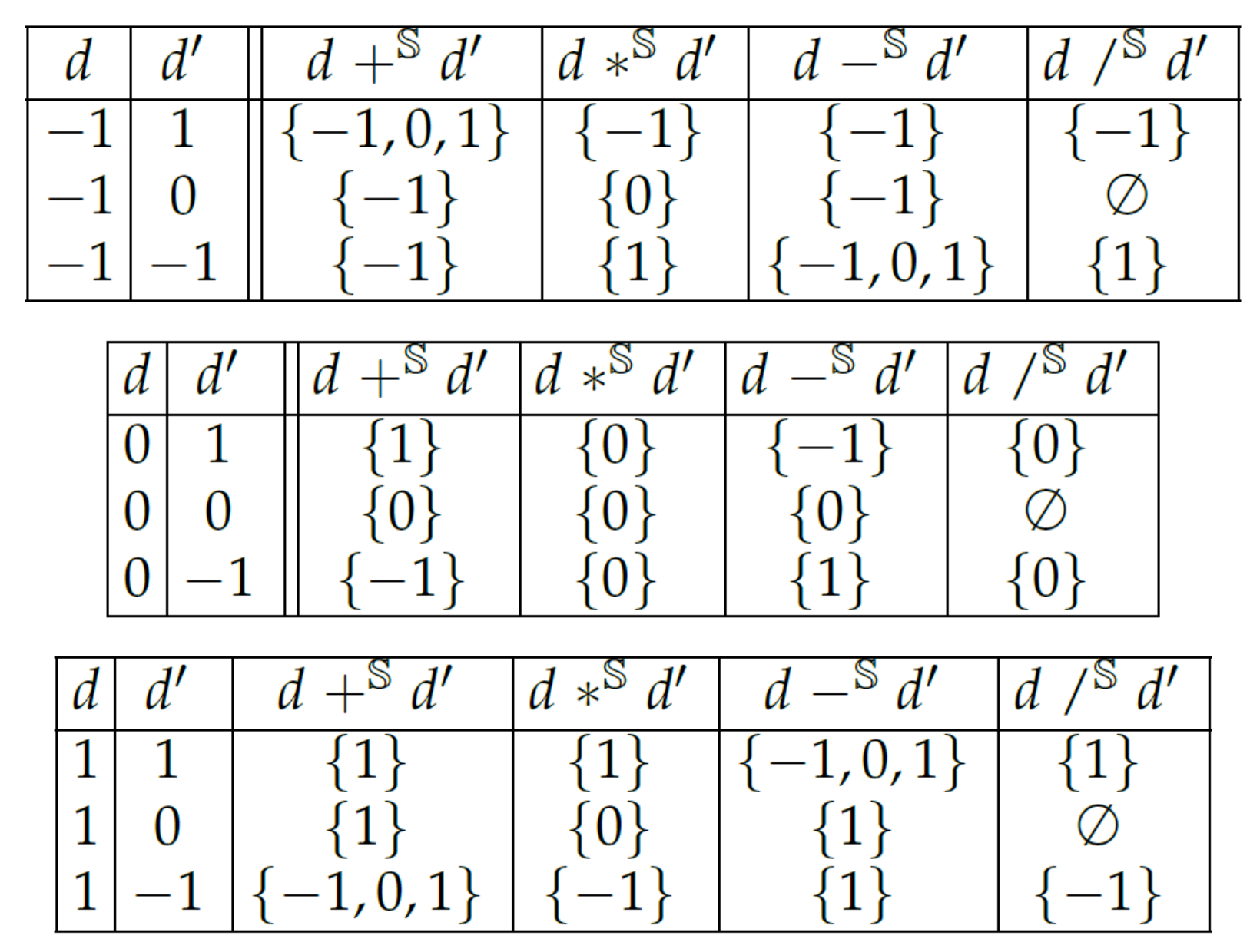
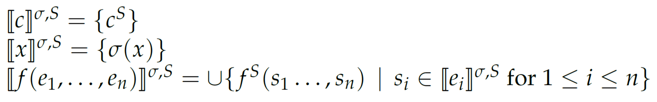
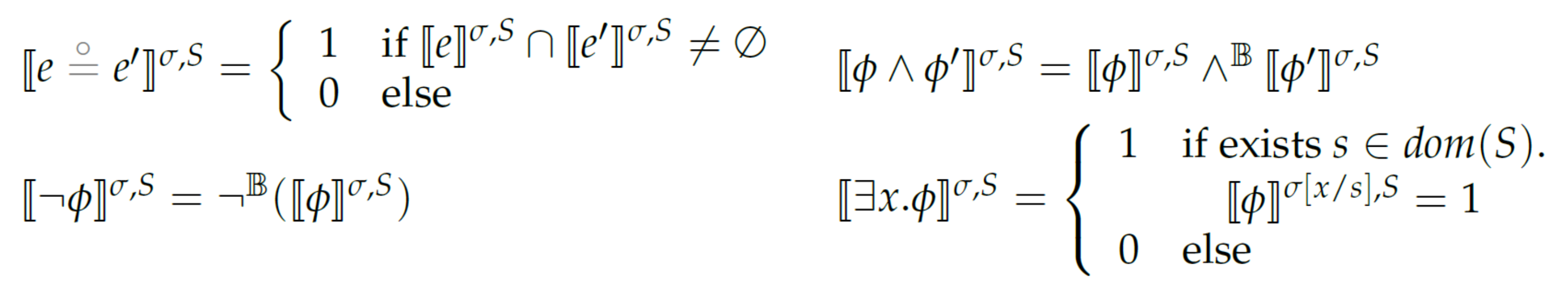
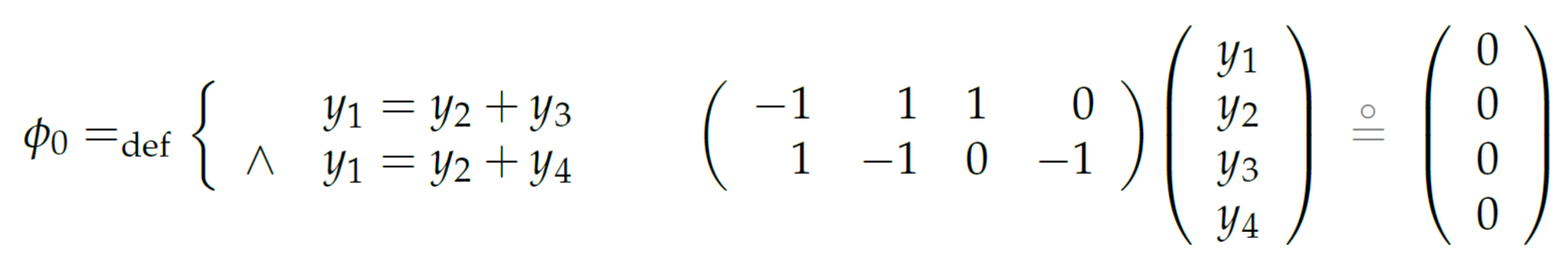
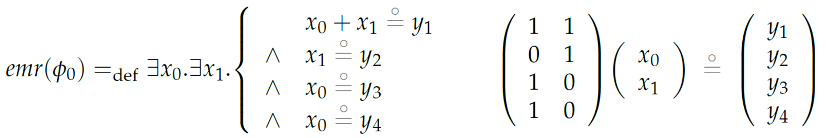
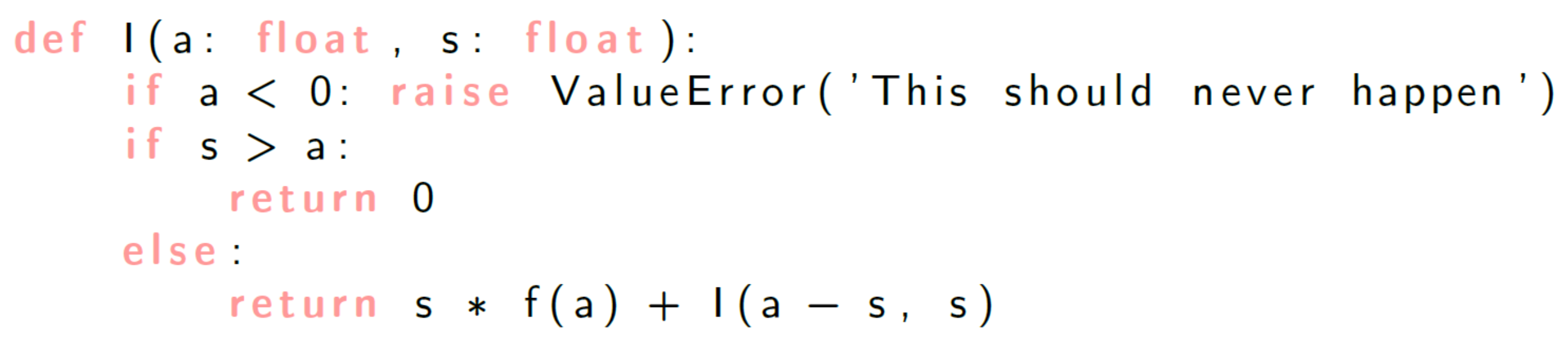
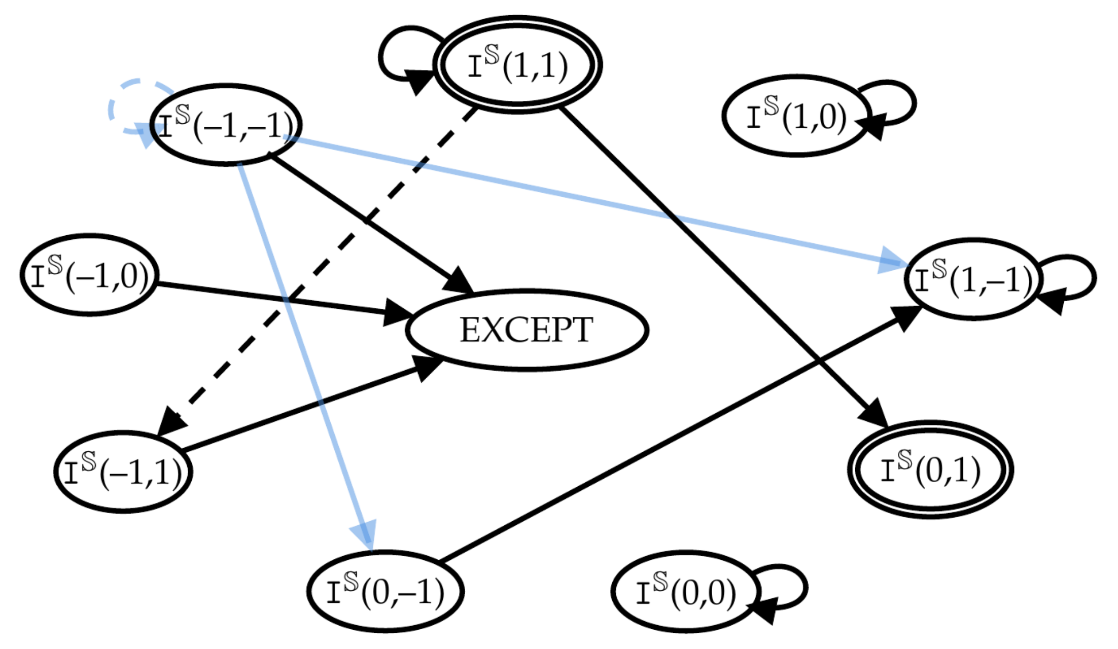
Table 1.
Set of abstract solutions in . Six solutions with gray background color are unjustified since outside .
Table 1.
Set of abstract solutions in . Six solutions with gray background color are unjustified since outside .
| # | ||||||
|---|---|---|---|---|---|---|
| 1. | 0 | 0 | 0 | 1 | −1 | 1 |
| 2. | 0 | 0 | 1 | 1 | 0 | 1 |
| 3. | 0 | 0 | 1 | 1 | −1 | 1 |
| 4. | 0 | 0 | 1 | 1 | 1 | 1 |
| 5. | 0 | 1 | 0 | 0 | 0 | 0 |
| 6. | 0 | 1 | 1 | 0 | 1 | 0 |
| 7. | 0 | 1 | 0 | −1 | 1 | −1 |
| 8. | 0 | 1 | 1 | 1 | 0 | 1 |
| 9. | 0 | 1 | 1 | −1 | 1 | −1 |
| 10. | 0 | 1 | 1 | 1 | −1 | 1 |
| 11. | 0 | 1 | 1 | 1 | 1 | 1 |
| 12. | 1 | 0 | −1 | 0 | −1 | 0 |
| 13. | 1 | 0 | −1 | −1 | 0 | −1 |
| 14. | 1 | 0 | −1 | −1 | −1 | −1 |
| 15. | 1 | 0 | −1 | −1 | 1 | −1 |
| 16. | 1 | 0 | −1 | 1 | −1 | 1 |
| 17. | 1 | 1 | −1 | −1 | 0 | −1 |
| 18. | 1 | 1 | −1 | −1 | −1 | −1 |
| 19. | 1 | 1 | −1 | −1 | 1 | −1 |
Publisher’s Note: MDPI stays neutral with regard to jurisdictional claims in published maps and institutional affiliations. |
© 2021 by the authors. Licensee MDPI, Basel, Switzerland. This article is an open access article distributed under the terms and conditions of the Creative Commons Attribution (CC BY) license (https://creativecommons.org/licenses/by/4.0/).
Share and Cite
MDPI and ACS Style
Allart, E.; Niehren, J.; Versari, C. Exact Boolean Abstraction of Linear Equation Systems. Computation 2021, 9, 113. https://0-doi-org.brum.beds.ac.uk/10.3390/computation9110113
AMA Style
Allart E, Niehren J, Versari C. Exact Boolean Abstraction of Linear Equation Systems. Computation. 2021; 9(11):113. https://0-doi-org.brum.beds.ac.uk/10.3390/computation9110113
Chicago/Turabian StyleAllart, Emilie, Joachim Niehren, and Cristian Versari. 2021. "Exact Boolean Abstraction of Linear Equation Systems" Computation 9, no. 11: 113. https://0-doi-org.brum.beds.ac.uk/10.3390/computation9110113
Note that from the first issue of 2016, this journal uses article numbers instead of page numbers. See further details here.