Video-Based Deep Learning Approach for 3D Human Movement Analysis in Institutional Hallways: A Smart Hallway

McGuirk, Connor J. C.; Baddour, Natalie; Lemaire, Edward D.

doi:10.3390/computation9120130

Open AccessArticle

Video-Based Deep Learning Approach for 3D Human Movement Analysis in Institutional Hallways: A Smart Hallway

by

Connor J. C. McGuirk

^1,2,*,

Natalie Baddour

¹

and

Edward D. Lemaire

^2,3

¹

Department of Mechanical Engineering, University of Ottawa, Ottawa, ON K1N 6N5, Canada

²

The Ottawa Hospital Research Institute, Ottawa, ON K1H 8M2, Canada

³

Faculty of Medicine, University of Ottawa, Ottawa, ON K1H 8M5, Canada

^*

Author to whom correspondence should be addressed.

Computation 2021, 9(12), 130; https://0-doi-org.brum.beds.ac.uk/10.3390/computation9120130

Submission received: 13 October 2021 / Revised: 22 November 2021 / Accepted: 22 November 2021 / Published: 2 December 2021

(This article belongs to the Section Computational Engineering)

Download

Browse Figures

Versions Notes

Abstract

:

New artificial intelligence- (AI) based marker-less motion capture models provide a basis for quantitative movement analysis within healthcare and eldercare institutions, increasing clinician access to quantitative movement data and improving decision making. This research modelled, simulated, designed, and implemented a novel marker-less AI motion-analysis approach for institutional hallways, a Smart Hallway. Computer simulations were used to develop a system configuration with four ceiling-mounted cameras. After implementing camera synchronization and calibration methods, OpenPose was used to generate body keypoints for each frame. OpenPose BODY25 generated 2D keypoints, and 3D keypoints were calculated and postprocessed to extract outcome measures. The system was validated by comparing ground-truth body-segment length measurements to calculated body-segment lengths and ground-truth foot events to foot events detected using the system. Body-segment length measurements were within 1.56 (SD = 2.77) cm and foot-event detection was within four frames (67 ms), with an absolute error of three frames (50 ms) from ground-truth foot event labels. This Smart Hallway delivers stride parameters, limb angles, and limb measurements to aid in clinical decision making, providing relevant information without user intervention for data extraction, thereby increasing access to high-quality gait analysis for healthcare and eldercare institutions.

Keywords:

Smart Hallway; artificial intelligence; motion analysis; marker-less; computer vision; 3D reconstruction; gait

1. Introduction

Motion analysis provides information and insights into the quality of movement for rehabilitation, performance analysis of professional athletes, and animation for video games or computer-generated imagery in movies. Of particular interest is improving the quality of information provided to healthcare professionals. Stride analysis and gait information are used in clinical decision making to optimally care for patients. Human motion analyses can aid in understanding rehabilitation progress [1], fall risk [1,2], progression of neurodegenerative diseases [3], and classifying gait patterns [4,5,6]. However, equipment, access, space, and human-resource requirements limit quantitative movement assessment within healthcare and eldercare environments. A Smart Hallway implementation could automatically record movement as a person walks through a hallway within an institution so that a therapist or physician can review walking parameters before their appointment. In an eldercare residence, movement data could be collected multiple times a day, thereby providing data to track changes in movement quality. Big data models could also be implemented to provide indicators for fall risk or dementia progression. The Smart Hallway design enables non-invasive data collection that would not interfere with existing hospital processes. These new capabilities rely on automated movement-data acquisition without human intervention.

A depth-camera approach for a Smart Hallway was created and validated by Gutta et al. [7]. Multiple Intel RealSense depth cameras were used to generate a point cloud of the person’s lower leg, processing the point-cloud-generated stride parameter outcome measures, which can be used for clinical decision making. Limitations of camera-person distance for accurate body digitization restricted the camera positioning to waist height along the hallway walls. This setup could lead to issues with camera obstruction and people hitting the cameras as they traverse the hallway in daily use.

A marker-less approach to human movement analysis could also utilize an array of RGB cameras, paired with an artificial intelligence model, to determine two-dimensional (2D) coordinates of a person’s major joints. The set of joint coordinates can then be used as point correspondences to create a three-dimensional (3D) skeleton reconstruction of the person. With these data, stride parameters and other biomechanical measurements can be extracted and used for clinical decision making [5,8]. Since data are extracted from video without requiring patient preparation or other interventions, this approach could eliminate many of the practical obstacles to implementing movement analysis in healthcare workflows.

Various marker-less motion-analysis systems have been reported. Labuguen et al. [9] implemented a four-camera system capturing 720p resolution and 30 frames per second (fps) to reconstruct 3D joint positions. OpenPose BODY25 was solely used to detect keypoints, and no tracking, filtering, or foot-event detection was implemented for full movement analysis. Results from this approach had a maximum average error of 7 cm on joint position. This system was also limited in its ability to track high-speed movements due to the low capture rate. Other methods implementing Microsoft Kinect^® sensors are limited in scalability due to each sensor requiring its own computer for processing [10]. Furthermore, depth-sensor approaches have significant noise when assessing foot-contact events and suffer from increasing depth-estimation errors at long ranges [7]. Due to the useable range of Kinect sensors, they typically must be kept close to the participant, as in the system implemented by Rodrigues et al. [10], where sensors were placed at waist level within two to three meters of the participant. This system utilized an array of Kinect sensors calibrated to each participant and synchronized at 35 fps. This method of calibration is too cumbersome to deploy for daily use and is therefore not adaptable to a Smart Hallway-type application. Methods that implement RGB camera arrays with pose-inference models have shown promising results for human motion analysis, such as the system implemented by Nakano et al. [11]. However, they did not implement proper synchronization methods or state-of-the-art calibration approaches needed to develop a useable system capable of producing semi-real-time results. Moreover, the Nakano et al. system does not automatically detect foot events and requires post-analysis of the data to segment strides, which is not useable for the Smart Hallway proposed in this paper. Overall, these existing marker-less motion-analysis approaches included some but not all the elements necessary for an automated Smart Hallway application. Table 1 details other approaches to the non-invasive motion-analysis problem. System error is not reported, as no standardized measure is used across all studies.

The goal of this research is to design, develop, and evaluate a marker-less motion-analysis system that provides movement-outcome measures for institutional hallway settings. The system must be non-invasive in its inherent design and provide a modular approach that is optimized and can be deployed in any institutional hallway setting. The system should also improve on past marker-less systems by providing a sufficient capture rate, a robust synchronization and calibration approach, and a method to automatically detect foot events and return common outcome measures. By implementing in an institutional hallway, the system would be accessible and enable movement analysis to be integrated into daily schedules. The ultimate goal for a “Smart Hallway” is to accurately and non-invasively assess and report a person’s human-movement status in an institutional setting, with minimal or no human intervention.

2. Materials and Methods

Motion-capture systems require a variety of components to work optimally in tandem. This research includes computer simulations to determine optimal camera layout, temporospatial synchronization validation, calibration validation, and evaluation with various walking scenarios. Appendix A, Appendix B and Appendix C provide details of optimal camera layout, temporospatial synchronization validation, calibration validation, and validation methods used to design the Smart Hallway.

Based on preliminary research [16], the open-source OpenPose BODY25 model was used for all body keypoint inferences. The OpenPose model was trained on a combination of the COCO and MPII pose datasets. OpenPose BODY25 produced accurate keypoint results from preliminary testing on clinically relevant movements [16]. These 2-dimensional (2D) points combine to create a skeleton model of the person of interest (Figure 1).

2.1. System Design Requirements

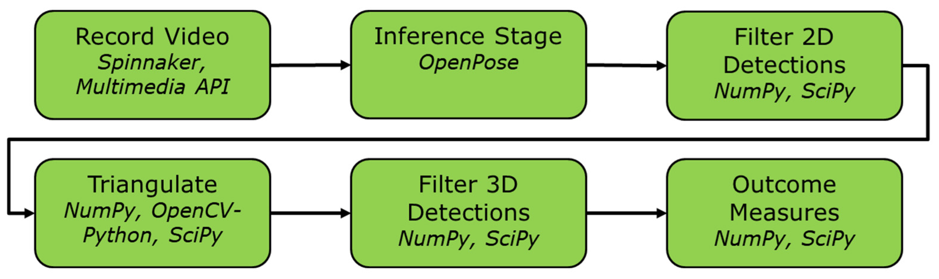
The Smart Hallway’s goal is to provide a non-invasive approach to extract gait outcome measures without human intervention. To effectively incorporate the system into hospital processes, the system must not interfere with individuals moving through the hallway [17]. Thus, typical hospital hallway dimensions were considered (length × 2.4 m × 2.8 m) when determining the placement of system components. The system components (cameras, cables, high-performance computing unit) should be mountable on the ceiling or high enough from the ground to not interfere with carts or people passing through. To extract data for 3D reconstruction using triangulation, at least two cameras are needed [18,19,20]. Increasing the number of cameras improves 3D reconstruction accuracy; this is a function of the camera-view overlap and number of detections of the point of interest, which can be passed to the optimization method. Based on simulation results, four cameras were used [8,21]. Other factors relating to 3D reconstruction accuracy include the camera resolution and synchronization. For the most accurate keypoint placement from OpenPose BODY25, the target must be at least 300 pixels tall in the camera frame [16,22]. Camera resolution is also dependent on the target-capture volume and lens specifications.

Camera synchronization is paramount for accurate reconstruction; having all cameras capture images at the same time reduces 3D reconstruction error. For this level of synchronization, a hardware approach with a stable sync signal is desirable. The system framerate is dependent on the type of motion being analyzed. For normal walking, a framerate of 60 fps is sufficient to reconstruct movement and extract useful outcome measures [23,24,25].

An accurate calibration routine for the camera array is required to extract accurate 3D information from the marker-less keypoints. Each camera’s projection matrix relative to the world origin contains variables for lens distortion, intrinsic parameters, and extrinsic parameters. These parameters are normally determined using a patterned calibration object and techniques such as Zhang’s method with random sample consensus (RANSAC) and bundle adjustment for camera extrinsic parameters [26,27,28]. These parameters should be calibrated such that the reprojection error is less than 1.0 pixel; however, this is dependent on camera resolution.

2.2. System Design

3D simulations were performed to determine the volumetric coverage achievable with four and eight cameras, respectively, within a hallway scenario. The simulated hallway was modelled as 5 m × 2.4 m × 2.8 m based on measurements from a typical hospital hallway. Selected components were modelled using Blender’s (Blender Foundation, Blender 2.91) camera object, and several iterations were performed while varying camera pose and placement relative to the world origin. The various configurations were compared based on parameters relating to capture volume that each setup produced (i.e., total capture volume, ground-area coverage, and view overlap). An array of four FLIR BlackFly^® S USB3 (BFS-U3-16S2C-CS) machine-vision cameras with Fujinon 3 MP Varifocal Lenses (YV4.3X2.8SA-2) were selected based on simulations. Figure 2 shows the virtual Smart Hallway camera layout, providing a 5 m × 2.4 m × 2.8 m (29 m³) capture volume with four cameras in an arc layout. Appendix A provides a detailed explanation of the simulation methods used.

System components were selected based on geometric and data-transfer constraints. Geometric constraints were based on the institutional hallway simulations and the maximum cable lengths for each communication standard (USB, GiGE, etc.). Data-transfer constraints were based on the desired multi-camera system performance in terms of resolution (minimum 960 × 720), pixel format (minimum 8 bit colour depth), and frame capture rate (minimum 60 fps). The selected components that best addressed the Smart Hallway requirements are detailed in Table 2.

A hardware synchronization cable was designed and created to ensure reliable image capture for the multi-camera system. A primary camera sends a sync signal at the beginning of exposure to the other cameras in the array, and the secondary cameras begin exposure once the sync signal has been received. This synchronization approach was validated by capturing 10,000 images and comparing the timestamps produced by each FLIR camera. The cameras remained synchronized within 5 μs of the primary camera when capturing at 60 fps (16,667 μs/image). This solution provides a repeatable synchronization method without the need for synchronization post data capture. Detailed cable design and validation methods are given in Appendix B for reproducibility.

Spatial synchronization for the multi-camera system was accomplished with a ChArUCo calibration pattern. Calibration was performed by capturing several views of the ChArUCo board and implementing OpenCV and Ceres libraries for robust camera parameter calculation. Final reprojection error from the distortion, intrinsic, and extrinsic parameters was less than 1.0 pixels. The multi-camera system calibration was tested by comparing system output to measured dimensions along the length of the capture volume (5 markers on the floor spaced at 1 m intervals). X-axis error was 1.7 (SD = 1.2) cm, Y-axis error was 2.4 (SD = 1.5) cm, and Z-axis error was 1.9 (SD = 1.4) cm. This solution allows for one-time system calibration that does not need to be performed prior to each data-collection session. The hardware pipeline is highlighted in Figure 3. Details of the calibration approach are given in Appendix C.

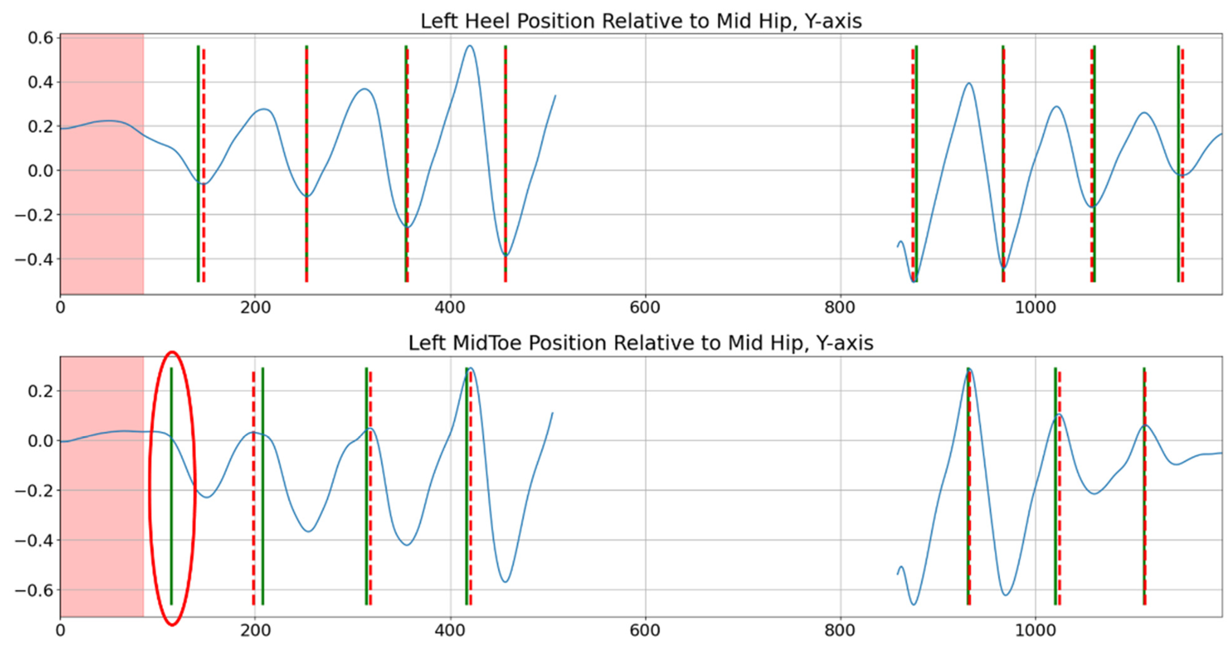
2.3. Signal Processing

Videos of participants were recorded and stored on the NVIDIA Jetson AGX’s solid-state drive. The videos were then passed to the OpenPose BODY25 model to perform inference and create a set of 2D keypoints, locating participant joint centres for every video frame. For every video, the 2D keypoint data contains confidence scores that describe the likelihood of correct marker location. Data from each video were preprocessed by removing points below 10% confidence and using a cubic spline to interpolate gaps in the dataset that are five frames (0.083 s) or less. The dataset was then filtered using a zero-phase low-pass 12 Hz Butterworth filter. Figure 4 shows an example of the 2D keypoint data after preprocessing.

2D keypoint data from each camera were passed to the triangulation pipeline, along with the intrinsic and extrinsic parameters. Point correspondences from the 2D keypoints were used in a non-linear optimization RANSAC triangulation method to determine an optimal set of 3D keypoints describing the body at each timestep in the video. For each trial’s 3D data, regions where 3D keypoint data reprojection error exceed two standard deviations from the mean were removed to reduce outlier effects.

Software was written in Python 3.7 to calculate body-segment lengths, stride parameters, and hip, knee, and ankle angles. 3D data were filtered using a zero-phase low-pass 5 Hz Butterworth filter, based on findings from other research involving OpenPose keypoint inferences and marker-based approaches [25,29].

Body-segment lengths were calculated using the Euclidean distance between limb endpoints. Body-segment lengths were measured at each timestep in the video. Measurements outside two standard deviations from the mean were identified as outliers and removed. For evaluation, body-segment length deltas were calculated as limb length subtracted from the measured limb length.

Ground-truth stride parameters were calculated from ground-truth foot events obtained by manually labelling foot offs and foot strikes in each video. Detected foot events were obtained by using the Zeni et al. algorithm [30]. The set of detected foot events was improved by implementing an algorithm to recover gait initiation and gait termination (initiation termination recovery, it recovery). Figure 5 shows an example of the detected foot events prior to the initiation and termination recovery algorithm.

Regions such as the one highlighted by the red ellipse in Figure 5 were recovered by searching the window between the stop region (red area) and the next detected foot event. The algorithm determined whether an initiation occurred by analyzing the linear fit of the curve in a calculated search region. The search region was assessed by detecting a potential foot event, using SciPy’s signal.find_peaks function, and fitting a line between the potential foot event and the next detected foot event [31]. Linear fits above an R-squared value of 0.85 were selected as gait initiations and added to the list of detected foot events. Foot events that were missed or not recovered by Zeni’s algorithm were backfilled using the algorithm proposed by Capela, Lemaire, and Baddour [32,33]. Algorithm 1 and Algorithm 2 describe the methods implemented by this research to detect foot events.

Algorithms 1 Method for detecting stops in a trial given an array of chest keypoint position per frame. Detect Stops.
0	Get first derivative of keypoints in chest keypoint array, A_C, smooth the array with a low-pass filter
1	get net average velocity of keypoints in the array V_N
2	set current stopped state to False
3	for index, point in A_C
4	create a sliding window on A_C of size K
5	get average velocity of the window V_W
6	if V_W less than V_N * scalar and current state is not stopped
7	current stop append frame index
8	stopped state to True
9	else if V_W greater than V_N * scalar and current state is stopped
10	current stop append frame index → S
11	S appended to S_N, current stop S set to empty list
12	stopped state to False
13	else pass
14	end
15	Return list of stops S_N

Algorithm 2 Method for detecting foot strikes during gait initiation and gait termination. Detect Foot Strikes.
0	create an empty event displacement array E ← [empty]
1	for index, point in foot/heel keypoint array, A_K
2	get heel keypoint displacement relative to the bottom chest keypoint
3	append the displacement data to E
4	smooth E with a low-pass filter
5	fine detect initial peaks in E as foot strikes F_S
6	pass E, F_S, and list of stop windows W_L to initiation/termination recovery method
7	for W in W_L
8	coarse detect peaks from E index 0 to start index of W
9	select the last detected peak as a potential gait termination strike P_S
10	create window between the last detected strike in F_{S r} and P_S
11	if last detected strike is equal to potential gait termination
12	Return is termination False
13	else
14	check concavity of the displacement data inside the newly constructed window W
15	construct a line L from the start to the end of W
16	determine the linear fit between the data inside W and L
17	if linear fit is less than threshold
18	Return is termination False
19	Return is termination True → P_S inserted in F_S

Processing time for foot-event detection and stride-parameter measurement was calculated using Python 3′s built in nanosecond clock. Foot-event detection took, on average, 18 ms for a 1500 frame trial. Stride-parameter measurement took an average of 35 ms for calculating 30 parameters across a 1500 frame trial.

Stride parameters included stride length, stride time, stride speed, step length, step width, step time, cadence, stance time, swing time, stance swing ratio, and double support time. Results for comparison included mean (

μ

) and standard deviation (

σ

) across all trials of the same walking condition for each participant.

Hip, knee, and ankle 3D angles for the left and right legs were calculated for each stride, defined by ground truth and detected foot events. Figure 6 shows how the vectors used in the angle calculations were defined. Hip angle was the angle between the torso vector and thigh vector, knee angle was the inner angle between the thigh and shank vector, and ankle angle was the inner angle between the shank and foot vector.

Figure 7 shows the final software pipeline of the Smart Hallway.

2.4. Validation

The Smart Hallway system was evaluated by testing two male participants (age: 28; height: 180 cm; weight: 64 kg and age: 25; height: 178 cm; weight: 90 kg). Each participant provided informed consent (University of Ottawa Ethics Board, H-01-21-5819). Data collection was completed in one testing session.

Prior to testing, each participant’s body-segment lengths were measured using an anthropometric tape. The segments matched OpenPose’s BODY25 model (Figure 1) and were measured by palpating the joint centres of interest for each measurement. Each participant completed five separate trials of five walking conditions (Table 3). Participants were recorded with the four-camera array at 60 fps. A total of 50 videos were recorded, containing approximately 500 foot events.

3. Results

From Table 4 and Table 5, mean differences between calculated and ground-truth values were small for the majority of body-segment lengths. In general, the calculated body-segment lengths were less than the ground-truth values. The average difference across all test conditions was 1.56 (SD = 2.77) cm. Since the delta results for participant one and participant two were similar, only the results for participant one were included in this manuscript. Results for participant two are located in Appendix D.

Table 6 shows the mean absolute error of the foot-event detection algorithms compared to ground-truth values obtained from manual labelling. The error in ground-truth labelling was three frames, and the average error in detected events across all trials was four frames. Table 7, Table 8, Table 9, Table 10 and Table 11, calculated stride parameters were comparable to ground-truth results.

Figure 8 shows the ensemble averaged leg angles during gait, from foot strike to foot off. The shape of the ankle, knee, and hip angle curves were similar to able-bodied joint angles from the literature [34].

4. Discussion

Based on the simulation, design, and evaluations from this research, marker-less human movement analysis is a viable option for outcome measurement of people moving within institutional hallways. The system configuration can lead to automated video capture and fully automated processing that enables outcome measurement with minimal or no human intervention. Unlike past research that has only tested the efficacy of marker-less human motion analysis, this work provides a fully implemented prototype that could be deployed in existing institutional environments and brings closer the adoption of marker-less motion analysis for use in practice.

Body-segment length measurements were within 1.56 (SD = 2.77) cm of ground-truth values. This is comparable to leg-length measurements used for clinical decision making, where the difference between Vicon limb lengths and X-Ray bone measurements was 0.98 (SD = 0.55) cm [35]. Stride parameters and joint angles were analyzed to determine the Smart Hallway’s capability for human motion analysis. Keypoint-based stride parameters were similar to ground-truth results. Across all test conditions, stride-parameter distances were 3.16 (SD = 3.26) cm from the ground truth. In all cases, the standard deviation of the delta was within the standard deviation of the calculated stride parameter. Stride-parameter times were 0.047 (SD = 0.037) s from the ground truth. The timing differences were very small and equivalent to the ground-truth foot-event timings. Stride-parameter velocities were 0.74 (SD = 0.75) cm/s from the ground truth. In particular, stride times for walking straight were 1.18 (SD = 0.05) s; this corresponds with findings from the literature, showing that the Smart Hallway’s standard deviation is within a similar range to existing marker-based gait datasets 1.02 (SD = 0.06) s [36].

Other studies analyzing physician ability for visual gait assessment concluded that raters had an average of 50% accuracy when compared to 3D marker data [37,38]. Even with such low accuracy, good clinical decision making is still possible, though some abnormal gait features are not detected during visual assessment [37,38,39]. Thus, the outcome measures calculated from the Smart Hallway can provide useful information for clinical decision making when compared to current visual assessment methods.

Stride parameters were affected by the walking aids; however, results were still similar to measures from the walking-straight condition. The ensemble average curves obtained from the leg-angle calculations showed similar shapes compared to leg angles from the literature [34].

Stride parameters that were only reliant on a single type of foot event (e.g., only left foot strikes) were highly accurate. Increased error and standard deviation in stride-parameter measurements were seen in parameters that relied on multiple types of foot events, including step length, step width, and stance-swing ratio. This is likely due to compounding errors by combining either contralateral foot events, foot strikes and foot offs, or foot events and 3D keypoint locations on the floor. Foot-event detection was within four frames (67 ms) of the ground-truth foot events. Stride parameters obtained using detected foot events were similar to stride parameters calculated using ground-truth foot events. More work is needed to improve foot-event detection accuracy when calculating stride parameters that rely on multiple data types, such as stance-swing ratio or contralateral step parameters.

Joint-angle standard deviations were greater when occlusions occurred or large variance existed in the Y depth coordinate between the keypoints of interest. Greater error in the global Y-axis is expected since this axis is related to scene depth and is sensitive to triangulation method accuracy. These occlusions and points of greater variance generally occurred at foot strike and foot off, where the leg is either at the maximum distance in front of the body or at the maximum distance behind the body, causing a greater variation in the Y-axis.

Smart Hallway accuracy was lower when keypoints were occluded by walking aids or the pose of the participant in the scene. Improvements can be made by increasing the number of cameras and implementing kinematic constraints on the BODY25 model to ensure that only realistic movements are produced in the 3D reconstruction. The current OpenPose BODY25 AI model does not account for physical and kinematic constraints such as consistent joint-to-joint segment lengths and range of motion of certain joints. Some recent approaches to keypoint-pose inference models, such as MotioNet, have included encodings for bone lengths and 3D joint rotation [40]. These models use a scaled estimation of the depth coordinate, which is learned through AI training processes that are also seen in Google ML Kit Pose Detection [41]. However, OpenPose BODY25 has better keypoint quality compared to these models.

The Smart Hallway produced viable results across all outcome measures, with low variance. For this prototype system, only two participants were recruited for testing; however, approximately 500 strides were analyzed in total. Improvements to the OpenPose BODY25 model or new, more advanced models should aid in more accurately detecting the feet and handling body-part occlusion. Currently, OpenPose processing is a system bottleneck, with results from a 10 s trial returned after approximately 120 s (NVIDIA Jetson AGX). Other processing stages, such as the triangulation step, could be further optimized to reduce data registration time. The current implementation is limited to handling one person in frame at a time; however, with upgrades to outcome-measurement software, groups of people could be processed since OpenPose BODY25 provides keypoints for all people in frame.

The Smart Hallway was successfully deployed in a manner that was non-invasive to the hallway environment. This implies that a system could be set up and gather data on multiple individuals that walk throughout the capture volume on a daily basis without obstructing existing institutional processes. The Smart Hallway system successfully captured data from individuals in a non-invasive manner that did not require markers or a data-collection device being affixed to the participants.

5. Conclusions

A Smart Hallway setup for marker-less 3D human motion analysis in institutional hallways was viable when using an array of four temporally and spatially synchronized cameras and OpenPose BODY25. Temporal synchronization was achieved for the multi-camera array, and spatial synchronization was achieved through a rigorous calibration procedure using RANSAC and bundle-adjustment techniques. 3D joint keypoints were successfully calculated from 50 videos (approximately 500 strides) that included straight walking, walking with turns, walking a curved path, using a walker, and using a cane. Body-segment lengths, foot events, and stride parameters from each condition were similar to manually identified and calculated ground-truth values. Ensemble averaged leg angles corresponded well with kinematic data from the literature [34]. The prototype system validated in this research allows for fully automated human motion analysis without the need for post-processing techniques for calibration, synchronization, or foot-event and stride-parameter analysis. This research helps to move human motion analysis from the lab to the point of patient contact by providing a full system design that is implementable in institutional settings but does not require extensive human resources for operation.

Future research could apply kinematic constraints to the reconstructed 3D results, such as consistent joint-to-joint segment lengths and constrained-joint range of motion in order to reconstruct only possible physical body positions. Furthermore, new training data or transfer learning, could be applied to make better inferences when movement aids are being used. Research into applying the Smart Hallway design to other areas of interest, such as gait-classification applications, could be performed to assess fall risk or neurodegenerative disease progression.

Author Contributions

Conceptualization, C.J.C.M., E.D.L. and N.B.; methodology, C.J.C.M., E.D.L. and N.B.; software, C.J.C.M.; validation, C.J.C.M.; formal analysis, C.J.C.M.; investigation, C.J.C.M.; resources, C.J.C.M., E.D.L. and N.B.; data curation, C.J.C.M.; writing—original draft preparation, C.J.C.M.; writing—review and editing, C.J.C.M., E.D.L. and N.B.; visualization, C.J.C.M.; supervision, E.D.L. and N.B.; project administration, E.D.L. and N.B.; funding acquisition, E.D.L. and N.B. All authors have read and agreed to the published version of the manuscript.

Funding

This research was funded by Natural Sciences and Engineering Research Council of Canada (NSERC), grant number RGPIN-2019-04106.

Institutional Review Board Statement

The study was conducted according to the guidelines of the Declaration of Helsinki and approved by the Research Ethics Board of the University of Ottawa (protocol code: H-01-21-5819 and date of approval: 08/02/2021).

Informed Consent Statement

Informed consent was obtained from all subjects involved in the study.

Data Availability Statement

Not applicable.

Acknowledgments

Graduate-student support was provided by the CREATE-READi program. The authors would like to thank The Ottawa Hospital Rehabilitation Centre and the University of Ottawa for providing resources for development and testing. They would also like to thank the volunteers who participated in this study.

Conflicts of Interest

The authors declare no conflict of interest.

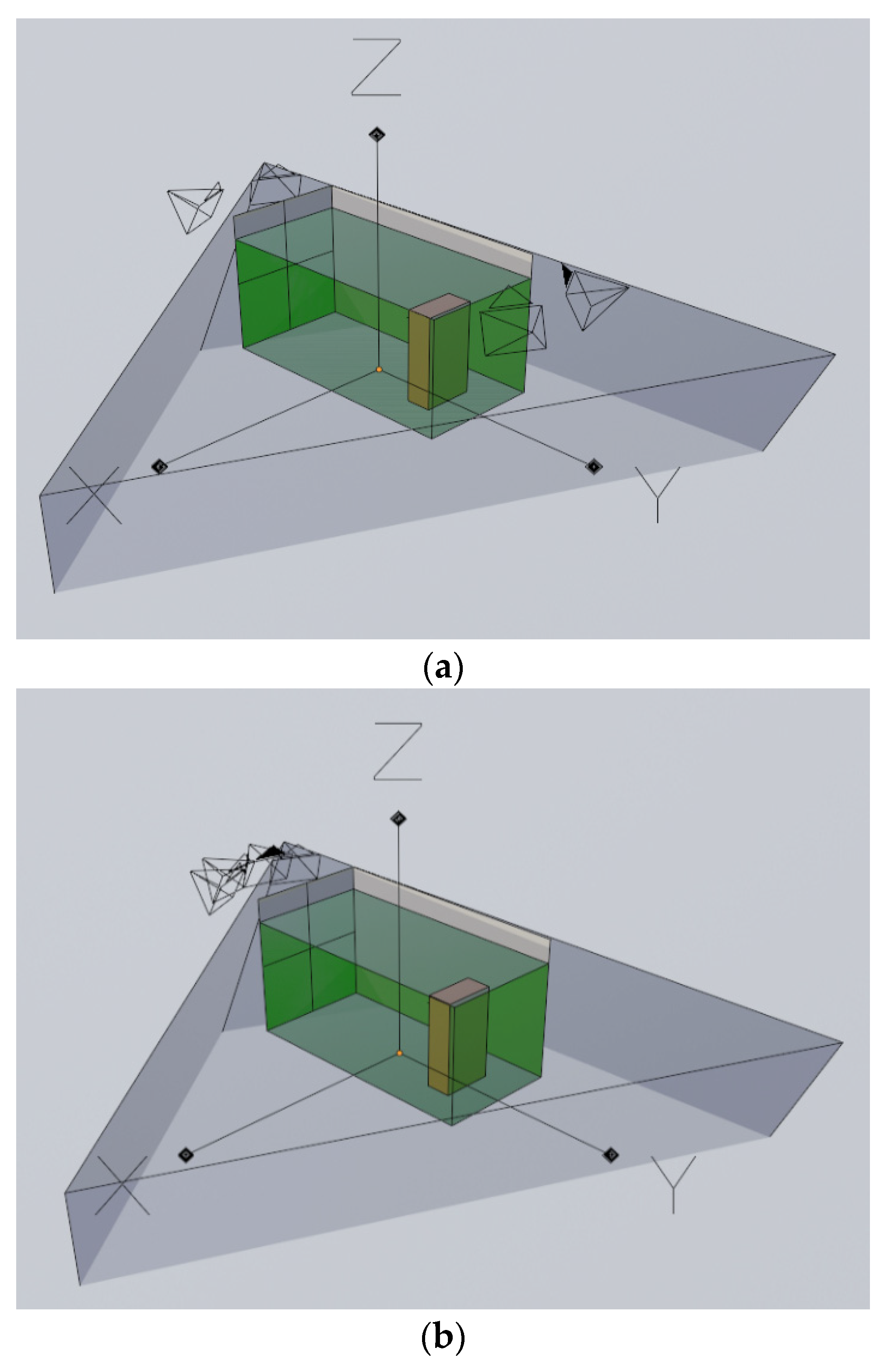
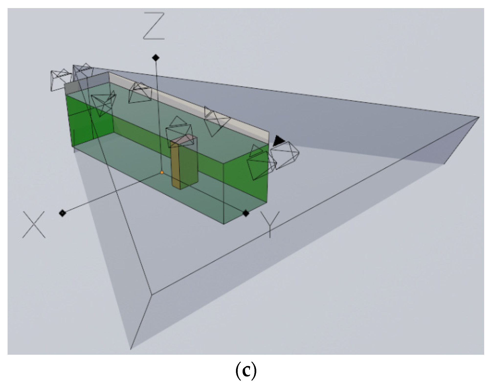
Appendix A. Simulation and Modelling

Appendix A.1. Methods

To simulate camera layout in order to achieve an optimal capture volume, with cameras located on the ceiling to avoid disrupting hallway access and people hitting the cameras, a method using Blender (Blender Foundation, Blender 2.91) to model the cameras was implemented [7]. Camera field of view (FoV) during simulation was 70° × 52.5°, based on lens specifications [42]. In this simulation, an arc layout and corner layout were evaluated. Setup 1 had four cameras, with one camera placed at each corner of the simulated hallway capture volume. Setup 2 had four cameras placed in an arc at one end of the simulated hallway. For each setup, three iterations were performed by adjusting camera poses. Both setup 1 and setup 2 aimed to capture a 5 m × 2.4 m × 2.5 m volume in the simulated hallway. Setup 3 had eight cameras placed equidistantly around a 10 m × 2.4 m × 2.5 capture volume to test how the system could scale to a greater number of cameras. For each setup, camera poses were varied to maximize FoV overlap and the percentage of useable volume. Useable volume was defined as the desired walking-distance length (5 m or 10 m), the width of the institutional hallway (2.4 m), and a conservative estimate of typical participant height (2.5 m). Figure A1 displays an example of the four-camera corner, four-camera arc, and eight-camera layouts.

Figure A1. Simulated camera layouts: (a) four-camera corner, (b) four-camera arc, (c) eight-camera perimeter.

Properties of the useable capture volume were calculated by determining the intersection of each camera’s respective FoV within the simulated hallway. A volume mesh describing the space in which all cameras have a view of the scene was formed from these intersections. Using Blender’s Boolean intersection method, several 3D meshes were produced and compared. The capture-volume meshes generated from each layout were compared to determine a camera layout that provided desirable features in the context of an institutional hallway setting. Individual camera capture volumes are defined in A1 as

C V_{i} = \frac{| \vec{A_{i} D_{i}} \times {\vec{A B}}_{i} | \cdot \vec{P_{i} A_{i}} \cdot (\vec{A_{i} D_{i}} \times \vec{A_{i} B_{i}})}{3 | \vec{A_{i} D_{i}} \times \vec{A_{i} B_{i}} |}

(A1)

with

C V

as the camera capture volume and

i

indicating the camera number in a multi-camera system. Vectors

[\vec{A_{i} B_{i}}, {\vec{A D}}_{i}, \vec{P_{i} A_{i}}]

are defined in Figure A2.

Figure A2. Vector definition of a single camera capture volume used to determine FoV intersections with multiple cameras.

The intersection of the camera volumes is defined in (A2) as

\sum_{i = 1}^{n} C V_{1} \cap C V_{i + 1} = \sum_{i = 1}^{n} {\vec{v} | \vec{v} \in C V_{1} a n d \vec{v} \in C V_{i + 1}}

(A2)

where

C V_{1}

defines the capture volume of camera 1,

C V_{i + 1}

defines the capture volumes of the other cameras in the multi-camera system, and

\vec{v}

defines the set of vectors that define each camera capture volume.

Appendix A.2. Validation

The total capture volume for each setup and the total ground-coverage areas are presented in Table A1. The capture-volume meshes (Figure A3) are shown for each layout with varying camera pitch angles. The four-camera arc layout provided more coverage of the simulated institutional hallway compared to the four-camera corner layout. For the four-camera corner layout, some stereo-camera pairs were too far apart to reliably achieve an accurate calibration. Additionally, 3D reconstruction accuracy for a given stereo-camera pair is dependent on the incidence angle between the two cameras [43]. The four-camera corner layout requires some pairs of stereo-cameras to exceed the desirable incidence angle, which could negatively affect the final 3D reconstruction accuracy. The eight-camera perimeter layout provided the best coverage overall (i.e., total capture volume, ground-coverage area). Increasing the number of cameras also improves the likelihood of more accurate 3D reconstruction. An optimization procedure could be performed to determine camera poses and placement based on capture volume, ground coverage, and the number of cameras to further improve these results.

Table A1. Capture volume and ground-coverage area from the simulated camera layouts. R is the range of camera poses in the X, Y, and Z axis for each camera layout.

Number of Cameras	Layout	Pitch Angle Variation (°)	Total Capture Volume (m³)	Ground-Coverage Area (m²)
4	Arc	R_x = [60°: 65°] R_y = 0° R_z = ±[12.5°, 25.0°]	34 (R_x = 65°) 31 (R_x = 62.5°) 29 (R_x = 60°)	10 (R_x = 65°) 11 (R_x = 62.5°) 11 (R_x = 60°)
4	Corner	R_x = [60°: 65°] R_y = 0° R_z = ±25.0°	33 (R_x = 65°) 30 (R_x = 62.5°) 28 (R_x = 60°)	8 (R_x = 65°) 10 (R_x = 62.5°) 11 (R_x = 60°)
8	Perimeter	R_x = [62.5°, 65°] R_y = 0° R_z = ±[12.5°, 25.0°]	61 (R_x = 62.5°)	20 (R_x = 62.5°)

Meshes obtained using the intersection procedure provided visual confirmation of the expected capture volume in the simulated institutional hallway. Geometric features of the capture-volume mesh could be used to obtain a desirable layout of the cameras and aid in camera positioning if certain features are desired. This may include maximizing the total volume, maximizing the camera capture-volume overlap, or minimizing the angle of incidence between cameras. Figure A3 shows the meshes obtained from the four-camera corner, four-camera arc, and eight-camera perimeter layouts.

Figure A3. Capture-volume meshes: (a) four-camera corner, (b) four-camera arc, (c) eight-camera perimeter.

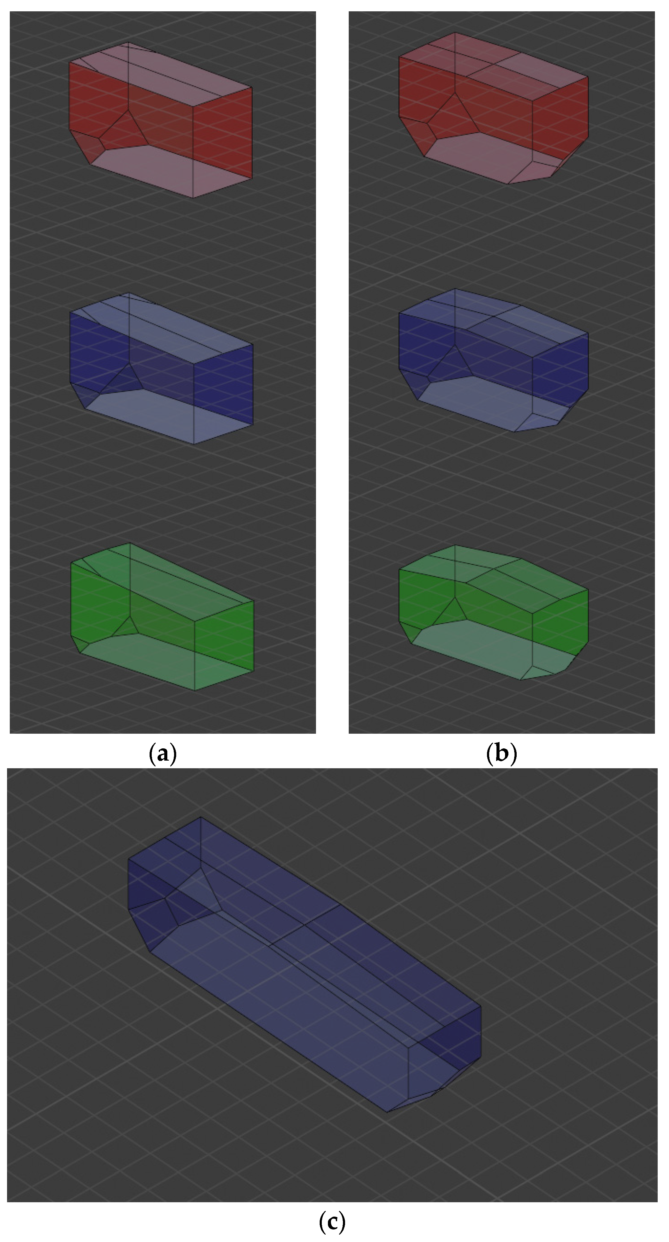
Appendix B. Camera Synchronization

Appendix B.1. Methods

FLIR BlackFly S USB3 cameras have a general-purpose input and output (GPIO) port that allows access to the camera auxiliary power input, auxiliary power ground, non-isolated input, and opto-isolated input. Camera software can be used to specify how GPIO will be used [44]. The hardware synchronization cable provided external power to the cameras while transferring the trigger signal produced by the primary camera. Cameras were powered externally to improve overall reliability and reduce the load on the NVIDIA Jetson AGX Xavier. The primary camera was formatted through software commands so that opto-isolated output produced a square wave as a function of the internal exposure time and selected frame rate. The secondary cameras were formatted similarly to the primary camera, except that the opto-isolated input was enabled to receive the primary camera’s trigger signal. To produce the desired trigger signal at the primary camera’s opto-isolated output, an external connection to a power source was required since the camera’s 3.3V input was occupied by the external camera power supply. Figure A4 displays connections to the primary and secondary camera GPIO ports.

Figure A4. Hardware synchronization cable GPIO pin connections for primary and secondary cameras.

The cable was built longer than necessary to accommodate the distance between cameras and variety of camera-array layouts tested. The distance between camera nodes was 7 m, and the connection to each camera was 0.75 m to allow for variability in placement. Due to the size of the cable and manufacturing capabilities, the external power connections were not consolidated into one connection and were not run alongside the trigger-signal wiring. Thus, camera power supplies were spliced into the cable near each camera GPIO connector. This is detailed in Figure A5, where the overall cable layout is shown, along with all connections.

Figure A5. Multi-camera synchronization cable expanded to an eight-camera setup.

Appendix B.2. Validation

Preliminary validation of the synchronization cable was performed by using a multimeter to measure current while running the cameras. Based on the inner circuitry of the opto-isolated GPIO, a 1.5 mA activation current was required at the LED to enable triggering [44] (opto-isolated output allows for a maximum current draw of 25 mA). The values in were measured using three different pull-up resistors at the primary camera.

Table A2. Current draw measurements while triggering multiple cameras. Activation current per camera must be >1.5 mA to enable triggering. Bolded values caused triggering to fail.

Pull-Up Resistor (kΩ)	Number of Cameras	Current Steady State (mA)	Current Active (mA)	Current Active (mA/Camera)	Trigger Success
2.4	2	4.73	3.01	1.55	Yes
	3	4.74	4.23	1.41	No
	4	4.74	4.37	1.09	No
1.2	2	9.06	3.56	1.78	Yes
	3	9.07	6.15	2.05	Yes
	4	9.08	7.84	1.96	Yes
0.6	6	18.10	11.88	1.98	Yes
0.6	8	18.11	15.44	1.93	Yes

To ensure cameras were being triggered properly, an oscilloscope was used to measure voltage changes at the output of the primary and input of the secondary cameras. Ideally, the signal produced by the primary camera should be identical to the signal received by each of the secondary cameras, without lag, to ensure that cameras are triggered at the same instant. Figure A6 shows the trigger wave, including the trigger and exposure portion of the signal.

Figure A6. Trigger signal produced by the primary (yellow) and received by the secondary (blue) cameras.

Once the trigger signal was validated, the lag between primary and secondary cameras was measured by capturing images (60 fps) of a millisecond clock (monitor refresh rate, 60 fps). A test using four cameras was performed, and after 167 s of image capture (10,000 frames), the final frame from each camera was compared. Figure A7 displays the setup and an example of the camera synchronization.

Figure A7. Synchronization test layout and validation images for a four-camera setup capturing at 60 fps. All cameras show the same frame of the millisecond clock after 10,000 images.

To further validate camera synchronization, image time stamps were converted to a standardized CPU time on the Jetson NVIDIA AGX Xavier. Three tests using four cameras capturing 10,000 synchronized images were performed to determine the robustness of the trigger-synchronization cable. Table 4 displays the average difference between the measured time stamp and the target 60 fps (16,667 μs/frame).

Table A3 shows the stability of the camera synchronization over 10,000 images and how closely in time the individual images are captured (on average). Camera positions were P: 20023229, S1: 20010192, S2: 20010189, and S3: 20010190.

Table A3. Timing differences between camera images during triggered image capture. Camera 20023229 (bolded) is the primary camera sending a trigger signal to each secondary camera. Timings were measured in nanoseconds and converted to microseconds.

	Image Timing Characteristics, Δ (μs)
Camera	μ	σ	σ²	Max Δ	Min Δ
20023229	0.00	0.39	0.16	4.00	−3.00
20010192	0.00	0.39	0.15	5.00	−5.00
20010190	0.04	0.56	0.32	5.00	−4.00
20010189	0.02	0.50	0.25	4.00	−5.00

Appendix C. System Calibration

Appendix C.1. Methods

Calibration of individual camera-intrinsic parameters and the multi-camera system’s extrinsic parameters was accomplished using a pattern calibration approach. The calibration pattern was an 8 × 7 ChArUCo board with a 4 × 4 (16 bit) dictionary of ArUCo random generator markers [45,46]. Chessboard squares were 110 mm, and ArUCo markers were 80 mm on each side.

For the intrinsic and extrinsic calibration process, a minimum of 200 images with a successfully detected calibration board were captured at a resolution of 1440 × 1080 pixels. The desired capture volume was outlined with markers to guide calibration and ensure that the entire volume was covered. During calibration, cameras were set to capture at 10 fps to reduce the total number of images passed to the ChArUCo board detection and calibration pipeline.

For intrinsic camera calibration, the set of images contained a variety of calibration-board poses that spanned a range of distances in the camera FoV. A RANSAC approach was used to determine each camera matrix and set of distortion coefficients [47]. After a set of images were captured for each camera, intrinsic calibration was performed using ChArUCo detection to obtain points on the calibration board and OpenCV’s extended library for access to the ChArUCo calibration functions. Images with poor reprojection error or too few detected ChArUCo markers were ignored during calibration. The calibration results were only accepted when a sufficiently low reprojection error was obtained from a given set of images (less than 1 pixel).

For extrinsic calibration, calibration-board images were captured from a variety of distances and angles relative to the cameras. For the extrinsic calibration process to successfully determine a valid rotation and translation between the camera pairs, the calibration board must be clearly visible in all images. Ideally, a quarter of the calibration board’s ChArUCo markers should be detected in an image to accurately determine calibration-board points. If too few markers are detected, the calibration-board points may have a poor reprojection error. For all frames with a partially detected ChArUCo calibration board, an image-point recovery algorithm was implemented to greatly increase the number of usable frames.

With a set of at least 200 successfully detected calibration boards, the calculated intrinsic parameter values were used to obtain an initial rotation matrix and translation vector connecting each secondary camera with the primary reference-frame camera. Initial extrinsic calibration results were only accepted when a reprojection error of less than 1 pixel was achieved. The set of extrinsic parameters was further improved using bundle adjustment, a modified version of OpenPose’s pipeline built using the Google Ceres library [48]. The modified bundle-adjustment approach utilizes some advantages of the ChArUCo calibration board to recover calibration points from images where only partial detections were obtained. Calibration was performed iteratively until the extrinsic-parameter pixel-reprojection error was less than 0.5 pixels.

For output-parameter calculations, the global coordinate system was transformed to the lab floor. An image of the calibration board on the ground was captured, and rotation and translation needed to transform the coordinate system to the board plane was calculated. This was performed multiple times with the board in a desired location to ensure that the new coordinate system’s X-axis lined up with the virtual capture volume width and that Y-axis aligned with the length.

Appendix C.2. Validation

Multi-camera system calibration was validated qualitatively and quantitatively. Qualitative assessment was performed by analyzing images from each camera to determine the effectiveness of the distortion model and by analyzing stereo-pairs of images to assess epipolar geometry characteristics. Removal of image distortions was verified by checking images for pin-cushioning or barrel distortion (Figure A8).

Figure A8. Barrel-distortion removal by camera-distortion model.

Figure A8 shows the removal of curvature caused by camera-lens distortion. Features such as the square calibration-board edges and ceiling-tile supports become straight in the undistorted view, as opposed to the distorted view.

Images from stereo-pairs of cameras were rectified and stitched together to determine whether epipolar constraints were violated. The epipolar constraint ensures that the projection of a given point from one image must lie on the epipolar line defined by the projected point and the imaging plane epipole of the other image. Points in the left camera view were tracked, along the corresponding epiline in the right camera, to ensure that the same point was found, with Figure A9 showing an example of a corner point in the left image being tracked along its epiline to the corresponding point in the right image.

Figure A9. Finding a point, P, in the left image and point, P′, in the right image along the same epiline to validate the epipolar constraint.

Quantitative validation was performed using the pixel-reprojection error obtained at each calibration stage. Final intrinsic-parameter-calibration results are documented in Table A4. The average extrinsic reprojection error was 0.21 pixels.

Table A4. Reprojection error in pixels after camera-intrinsic and -extrinsic parameter calibration.

Camera ID	Intrinsic Reprojection Error (Pixels)
20010190	0.64
20023191	0.52
20023230	0.51
20023235	0.48

A pixel-reprojection error of less than 1 pixel is generally desirable; however, this can vary depending on the image-sensor resolution. The average error after intrinsic-parameter calibration was less than 1 pixel for all cameras, and the overall average reprojection error calculated during the extrinsic-parameter bundle adjustment was 0.21 pixels.

The depth accuracy of the calibrated multi-camera system was tested by measuring the capture volume length, width, and height. These values were obtained by selecting corresponding points in each camera view by placing markers on the ground or ceiling. The point correspondences were then passed to the triangulation pipeline to determine measures of the capture-volume dimensions.

The triangulation pipeline was written in Python 3.7 and used code from the AniposeLib GitHub repository as a structure for the triangulation procedure [49,50]. The triangulation procedure used for the Smart Hallway applied a RANSAC approach to remove outliers in the detected points. The selected points were then triangulated using a bundle-adjustment approach, where the final 3D keypoint was iteratively adjusted to reduce the overall reprojection error in each camera view.

After verifying the final calibration, the measured capture-volume length was 5.04 ± 0.015 m, the width was 2.42 ± 0.012 m, and the height was 3.02 ± 0.014 m.

Appendix D

Table A5. Body-segment lengths for participant two: walking-straight, walking-turn, and walker-curve conditions (mean and standard deviation in brackets). Smart Hallway (SH) is calculated using the 3D reconstructed data, and Delta is the difference between the Smart Hallway and ground-truth segment length.

	Walking Straight		Walking Turn		Walking Curve
Limb Segment (cm)	SH	Delta	SH	Delta	SH	Delta
Left Arm	29.27 (1.69)	1.77 (1.69)	29.19 (1.36)	1.69 (1.36)	29.10 (1.40)	1.60 (1.40)
Left Forearm	27.56 (3.22)	0.56 (3.22)	25.97 (2.88)	−1.03 (2.88)	26.29 (1.82)	−0.71 (1.82)
Right Arm	30.19 (3.80)	2.69 (3.80)	28.80 (1.62)	1.30 (1.62)	29.17 (1.20)	1.67 (1.20)
Right Forearm	26.68 (2.90)	−0.32 (2.90)	25.94 (2.84)	−1.06 (2.84)	25.54 (1.73)	−1.46 (1.73)
Left Thigh	41.54 (2.44)	−2.46 (2.44)	41.65 (2.85)	−2.35 (2.85)	40.94 (1.94)	−3.06 (1.94)
Left Shank	42.49 (3.81)	0.99 (3.81)	42.66 (3.34)	1.16 (3.34)	42.98 (2.92)	1.48 (2.92)
Right Thigh	41.87 (3.09)	−2.63 (3.09)	41.43 (2.50)	−3.07 (2.50)	41.12 (2.00)	−3.38 (2.00)
Right Shank	41.75 (4.09)	0.25 (4.09)	42.51 (3.70)	1.01 (3.70)	42.13 (3.02)	0.63 (3.02)
Left Ankle to Heel	7.67 (2.54)	−0.33 (2.54)	7.02 (2.26)	−0.98 (2.26)	7.00 (1.88)	−1.00 (1.88)
Left Ankle to Big Toe	16.06 (4.26)	−3.44 (4.26)	16.63 (4.60)	−2.87 (4.60)	17.10 (3.13)	−2.40 (3.13)
Left Ankle to Small Toe	14.38 (3.90)	−2.12 (3.90)	15.96 (4.06)	−0.54 (4.06)	16.00 (3.47)	−0.50 (3.47)
Left Toe Width	7.05 (2.46)	−1.95 (2.46)	8.00 (3.27)	−1.00 (3.27)	7.05 (2.58)	−1.95 (2.58)
Right Ankle to Heel	7.20 (3.33)	-0.80 (3.33)	7.36 (2.21)	−0.64 (2.21)	10.50 (4.47)	2.50 (4.47)
Right Ankle to Big Toe	17.09 (3.67)	−2.91 (3.67)	16.98 (4.04)	−3.02 (4.04)	17.24 (2.82)	−2.76 (2.82)
Right Ankle to Small Toe	15.68 (3.80)	−0.82 (3.80)	14.56 (3.16)	−1.94 (3.16)	15.20 (2.66)	−1.30 (2.66)
Right Toe Width	7.29 (2.58)	−1.21 (2.58)	8.90 (3.41)	0.40 (3.41)	7.76 (3.89)	−0.74 (3.89)
Shoulder Width	33.18 (1.46)	−0.82 (1.46)	32.50 (1.24)	−1.50 (1.24)	32.67 (1.61)	−1.33 (1.61)
Hip Width	20.71 (1.28)	−0.29 (1.28)	20.83 (1.46)	−0.17 (1.46)	20.93 (1.89)	−0.07 (1.89)
Chest Height	52.93 (1.34)	−3.07 (1.34)	52.32 (1.72)	−3.68 (1.72)	53.26 (1.39)	−2.74 (1.39)

Table A6. Body-segment lengths for participant two: walking-straight, cane, and walker test conditions (mean and standard deviation in brackets). Smart Hallway (SH) is calculated using the 3D reconstructed data, and Delta is the difference between the Smart Hallway and ground-truth segment length.

	Walking Straight		Cane		Walker
Limb Segment (cm)	SH	Delta	SH	Delta	SH	Delta
Left Arm	29.27 (1.69)	1.77 (1.69)	29.42 (1.72)	1.92 (1.72)	29.09 (1.60)	1.59 (1.60)
Left Forearm	27.56 (3.22)	0.56 (3.22)	26.31 (1.57)	−0.69 (1.57)	28.88 (3.90)	1.88 (3.90)
Right Arm	30.19 (3.80)	2.69 (3.80)	29.60 (1.90)	2.10 (1.90)	29.42 (1.98)	1.92 (1.98)
Right Forearm	26.68 (2.90)	−0.32 (2.90)	27.42 (3.64)	0.42 (3.64)	28.02 (3.55)	1.02 (3.55)
Left Thigh	41.54 (2.44)	−2.46 (2.44)	40.75 (2.48)	−3.25 (2.48)	41.44 (3.09)	−2.56 (3.09)
Left Shank	42.49 (3.81)	0.99 (3.81)	42.38 (2.97)	0.88 (2.97)	43.56 (3.39)	2.06 (3.39)
Right Thigh	41.87 (3.09)	−2.63 (3.09)	41.26 (3.15)	−3.24 (3.15)	40.89 (3.03)	−3.61 (3.03)
Right Shank	41.75 (4.09)	0.25 (4.09)	41.85 (3.52)	0.35 (3.52)	42.93 (3.53)	1.43 (3.53)
Left Ankle to Heel	7.67 (2.54)	−0.33 (2.54)	7.08 (2.21)	−0.92 (2.21)	6.80 (2.21)	−1.20 (2.21)
Left Ankle to Big Toe	16.06 (4.26)	−3.44 (4.26)	17.59 (4.52)	−1.91 (4.52)	15.67 (3.68)	−3.83 (3.68)
Left Ankle to Small Toe	14.38 (3.90)	−2.12 (3.90)	15.27 (4.39)	−1.23 (4.39)	13.31 (4.15)	−3.19 (4.15)
Left Toe Width	7.05 (2.46)	−1.95 (2.46)	6.96 (2.62)	−2.04 (2.62)	7.53 (2.64)	−1.47 (2.64)
Right Ankle to Heel	7.20 (3.33)	−0.80 (3.33)	6.13 (2.08)	−1.87 (2.08)	7.09 (2.44)	−0.91 (2.44)
Right Ankle to Big Toe	17.09 (3.67)	−2.91 (3.67)	16.84 (4.34)	−3.16 (4.34)	17.09 (3.86)	−2.91 (3.86)
Right Ankle to Small Toe	15.68 (3.80)	−0.82 (3.80)	14.57 (3.60)	−1.93 (3.60)	14.75 (3.59)	−1.75 (3.59)
Right Toe Width	7.29 (2.58)	−1.21 (2.58)	7.70 (2.87)	−0.80 (2.87)	7.73 (2.75)	−0.77 (2.75)
Shoulder Width	33.18 (1.46)	−0.82 (1.46)	33.62 (2.07)	−0.38 (2.07)	33.57 (1.84)	−0.43 (1.84)
Hip Width	20.71 (1.28)	−0.29 (1.28)	20.58 (1.51)	−0.42 (1.51)	20.63 (1.21)	−0.37 (1.21)
Chest Height	52.93 (1.34)	−3.07 (1.34)	52.56 (1.15)	−3.44 (1.15)	54.13 (2.43)	−1.87 (2.43)

Table A7. Stride parameters for participant two: walking-straight test (mean and standard deviation in brackets).

	Left			Right
Parameters (Units)	SH	Ground Truth	Delta	SH	Ground Truth	Delta
Stride length (m)	1.48 (0.15)	1.50 (0.13)	0.01 (0.07)	1.48 (0.17)	1.47 (0.15)	−0.01 (0.08)
Stride time (s)	1.13 (0.08)	1.14 (0.07)	0.01 (0.03)	1.18 (0.21)	1.17 (0.19)	−0.01 (0.05)
Stride speed (m/s)	1.31 (0.16)	1.32 (0.15)	0.00 (0.04)	1.26 (0.17)	1.26 (0.17)	0.00 (0.03)
Step length (m)	0.45 (0.15)	0.32 (0.12)	−0.14 (0.05)	0.45 (0.17)	0.35 (0.13)	−0.10 (0.06)
Step width (m)	0.07 (0.04)	0.08 (0.04)	0.01 (0.00)	0.08 (0.04)	0.09 (0.03)	0.01 (0.02)
Step time (s)	0.59 (0.11)	0.58 (0.08)	−0.01 (0.05)	0.57 (0.05)	0.57 (0.05)	0.01 (0.04)
Cadence (steps/min)	101.94 (8.36)	103.40 (5.93)	1.46 (4.14)	103.68 (13.56)	103.83 (13.47)	0.14 (4.55)
Stance time (s)	0.69 (0.05)	0.74 (0.07)	0.05 (0.06)	0.70 (0.07)	0.72 (0.04)	0.02 (0.06)
Swing time (s)	0.45 (0.06)	0.42 (0.02)	−0.03 (0.06)	0.48 (0.08)	0.42 (0.03)	−0.06 (0.07)
Stance swing ratio (NA)	1.53 (0.19)	1.75 (0.11)	0.22 (0.25)	1.47 (0.28)	1.71 (0.10)	0.24 (0.29)
Double support time (s)	0.12 (0.03)	0.16 (0.04)	0.04 (0.05)	0.13 (0.05)	0.16 (0.04)	0.03 (0.06)
Foot angle (°)	12.63 (6.90)	12.45 (6.97)	−0.18 (0.07)	21.15 (9.33)	20.33 (8.49)	−0.81 (2.02)

Table A8. Stride parameters for participant two: walking-turn test (mean and standard deviation in brackets).

	Left			Right
Parameters (Units)	Measured	Ground Truth	Delta	Measured	Ground Truth	Delta
Stride length (m)	1.56 (0.20)	1.54 (0.19)	−0.02 (0.08)	1.55 (0.21)	1.53 (0.24)	−0.02 (0.10)
Stride time (s)	1.05 (0.10)	1.03 (0.10)	−0.02 (0.08)	1.04 (0.07)	1.04 (0.08)	0.00 (0.05)
Stride speed (m/s)	1.45 (0.24)	1.47 (0.20)	0.02 (0.05)	1.51 (0.22)	1.49 (0.22)	−0.02 (0.05)
Step length (m)	0.40 (0.13)	0.35 (0.12)	−0.05 (0.04)	0.41 (0.13)	0.37 (0.12)	−0.04 (0.04)
Step width (m)	0.08 (0.05)	0.09 (0.05)	0.01 (0.03)	0.11 (0.05)	0.12 (0.05)	0.01 (0.02)
Step time (s)	0.54 (0.13)	0.53 (0.13)	0.00 (0.08)	0.52 (0.09)	0.51 (0.07)	−0.01 (0.07)
Cadence (steps/min)	109.03 (7.18)	109.67 (7.33)	0.64 (4.73)	112.03 (2.41)	112.92 (3.49)	0.89 (4.79)
Stance time (s)	0.62 (0.10)	0.62 (0.09)	0.00 (0.07)	0.62 (0.10)	0.62 (0.09)	0.00 (0.07)
Swing time (s)	0.42 (0.08)	0.40 (0.07)	−0.02 (0.10)	0.42 (0.08)	0.40 (0.07)	−0.02 (0.10)
Stance swing ratio (NA)	1.54 (0.53)	1.56 (0.32)	0.02 (0.57)	1.54 (0.53)	1.56 (0.32)	0.02 (0.57)
Double support time (s)	0.12 (0.13)	0.14 (0.11)	0.01 (0.05)	0.13 (0.13)	0.14 (0.11)	0.01 (0.05)
Foot angle (°)	14.21 (6.84)	13.95 (6.87)	−0.26 (1.65)	14.21 (6.84)	13.95 (6.87)	−0.26 (1.65)

Table A9. Stride parameters for participant two: walking-curve test (mean and standard deviation in brackets).

	Left			Right
Parameters (Units)	Measured	Ground Truth	Delta	Measured	Ground Truth	Delta
Stride length (m)	1.36 (0.23)	1.37 (0.16)	0.02 (0.12)	1.27 (0.20)	1.26 (0.19)	−0.01 (0.12)
Stride time (s)	1.03 (0.10)	1.04 (0.06)	0.01 (0.06)	1.06 (0.07)	1.05 (0.05)	−0.01 (0.05)
Stride speed (m/s)	1.31 (0.15)	1.32 (0.13)	0.01 (0.06)	1.22 (0.12)	1.22 (0.11)	0.00 (0.04)
Step length (m)	0.37 (0.12)	0.27 (0.10)	−0.09 (0.05)	0.35 (0.18)	0.28 (0.14)	−0.07 (0.05)
Step width (m)	0.27 (0.15)	0.22 (0.14)	−0.05 (0.07)	0.31 (0.18)	0.27 (0.15)	−0.04 (0.04)
Step time (s)	0.51 (0.10)	0.50 (0.07)	−0.01 (0.06)	0.53 (0.05)	0.54 (0.05)	0.01 (0.05)
Cadence (steps/min)	115.62 (9.07)	118.48 (7.58)	2.85 (7.42)	110.18 (8.01)	110.78 (5.57)	0.59 (5.09)
Stance time (s)	0.62 (0.08)	0.65 (0.04)	0.04 (0.06)	0.64 (0.06)	0.65 (0.05)	0.01 (0.04)
Swing time (s)	0.41 (0.08)	0.39 (0.05)	−0.03 (0.05)	0.43 (0.09)	0.41 (0.05)	−0.02 (0.06)
Stance swing ratio (NA)	1.48 (0.31)	1.64 (0.12)	0.16 (0.28)	1.46 (0.37)	1.58 (0.24)	0.12 (0.22)
Double support time (s)	0.12 (0.05)	0.13 (0.03)	0.01 (0.05)	0.11 (0.04)	0.12 (0.02)	0.01 (0.04)
Foot angle (°)	35.63 (17.17)	37.41 (17.72)	1.77 (3.14)	34.81 (18.50)	36.20 (18.90)	1.38 (3.08)

Table A10. Stride parameters for participant two: cane test (mean and standard deviation in brackets).

	Left			Right
Parameters (Units)	Measured	Ground Truth	Delta	Measured	Ground Truth	Delta
Stride length (m)	1.65 (0.19)	1.64 (0.20)	−0.01 (0.05)	1.68 (0.20)	1.70 (0.18)	0.02 (0.10)
Stride time (s)	1.58 (0.10)	1.56 (0.12)	−0.02 (0.06)	1.58 (0.08)	1.58 (0.09)	0.00 (0.05)
Stride speed (m/s)	1.05 (0.11)	1.05 (0.11)	0.00 (0.01)	1.09 (0.11)	1.09 (0.11)	−0.01 (0.02)
Step length (m)	0.47 (0.20)	0.46 (0.20)	−0.01 (0.03)	0.54 (0.16)	0.49 (0.15)	-0.06 (0.04)
Step width (m)	0.06 (0.03)	0.06 (0.03)	0.00 (0.01)	0.08 (0.03)	0.08 (0.03)	0.00 (0.01)
Step time (s)	0.75 (0.07)	0.79 (0.07)	0.04 (0.05)	0.82 (0.09)	0.77 (0.09)	−0.05 (0.07)
Cadence (steps/min)	80.48 (7.55)	77.32 (5.83)	−3.16 (4.63)	73.37 (5.79)	78.08 (6.17)	4.70 (5.13)
Stance time (s)	0.95 (0.07)	0.92 (0.06)	−0.03 (0.08)	0.93 (0.09)	0.96 (0.07)	0.03 (0.07)
Swing time (s)	0.63 (0.09)	0.63 (0.09)	0.00 (0.08)	0.65 (0.09)	0.59 (0.08)	−0.05 (0.07)
Stance swing ratio (NA)	1.51 (0.21)	1.44 (0.16)	−0.07 (0.19)	1.45 (0.21)	1.64 (0.21)	0.18 (0.28)
Double support time (s)	0.18 (0.07)	0.18 (0.03)	−0.01 (0.07)	0.13 (0.05)	0.14 (0.03)	0.01 (0.05)
Foot angle (°)	13.50 (7.01)	13.40 (7.01)	−0.10 (0.57)	15.22 (3.39)	14.92 (3.80)	−0.30 (1.13)

Table A11. Stride parameters for participant two: walker test (mean and standard deviation in brackets).

	Left			Right
Parameters (Units)	Measured	Ground Truth	Delta	Measured	Ground Truth	Delta
Stride length (m)	1.01 (0.22)	1.01 (0.23)	0.00 (0.06)	1.02 (0.20)	1.01 (0.19)	−0.01 (0.06)
Stride time (s)	1.78 (0.13)	1.79 (0.14)	0.00 (0.10)	1.81 (0.18)	1.80 (0.14)	−0.01 (0.08)
Stride speed (m/s)	0.57 (0.13)	0.57 (0.13)	0.00 (0.01)	0.57 (0.13)	0.57 (0.13)	0.00 (0.01)
Step length (m)	0.33 (0.15)	0.30 (0.16)	−0.03 (0.04)	0.30 (0.15)	0.29 (0.16)	−0.02 (0.03)
Step width (m)	0.06 (0.04)	0.07 (0.04)	0.01 (0.01)	0.11 (0.04)	0.11 (0.04)	0.00 (0.01)
Step time (s)	0.90 (0.18)	0.88 (0.16)	−0.02 (0.08)	0.91 (0.13)	0.92 (0.14)	0.01 (0.07)
Cadence (steps/min)	66.09 (8.17)	68.15 (7.68)	2.06 (2.42)	66.81 (7.72)	66.13 (7.58)	−0.68 (4.17)
Stance time (s)	1.13 (0.10)	1.20 (0.12)	0.06 (0.12)	1.16 (0.14)	1.20 (0.11)	0.04 (0.09)
Swing time (s)	0.67 (0.13)	0.59 (0.09)	−0.08 (0.12)	0.63 (0.09)	0.59 (0.07)	−0.04 (0.09)
Stance swing ratio (NA)	1.70 (0.28)	1.94 (0.24)	0.24 (0.39)	1.84 (0.31)	1.99 (0.23)	0.15 (-0.08)
Double support time (s)	0.23 (0.08)	0.29 (0.07)	0.06 (0.10)	0.25 (0.10)	0.31 (0.09)	0.06 (0.13)
Foot angle (°)	14.55 (5.73)	14.60 (5.84)	0.06 (0.78)	15.25 (4.82)	15.25 (4.76)	0.01 (2.88)

Figure A10. Ensemble averaged leg angles measured by the Smart Hallway towards the camera array (row (A)) and away from the camera array (row (B)). Comparator data [34] (row (C)) show similar shape and range of motion. Grey dotted lines are the one-standard-deviation upper.

References

Anishchenko, L. Machine learning in video surveillance for fall detection. In Ural Symposium on Biomedical Engineering, Radioelectronics and Information Technology (USBEREIT); IEEE: Manhattan, NY, USA, 2018; pp. 99–102. [Google Scholar] [CrossRef]
Jenpoomjai, P.; Wosri, P.; Ruengittinun, S.; Hu, C.-L.; Chootong, C. VA Algorithm for Elderly’s Falling Detection with 2D-Pose-Estimation. In Proceedings of the 2019 Twelfth International Conference on Ubi-Media Computing (Ubi-Media), Bali, Indonesia, 6–9 August 2019; pp. 236–240. [Google Scholar] [CrossRef]
Taylor, M.E.; Delbaere, K.; Mikolaizak, A.S.; Lord, S.R.; Close, J.C. Gait parameter risk factors for falls under simple and dual task conditions in cognitively impaired older people. Gait Posture 2013, 37, 126–130. [Google Scholar] [CrossRef]
Tao, W.; Liu, T.; Zheng, R.; Feng, H. Gait Analysis Using Wearable Sensors. Sensors 2012, 12, 2255–2283. [Google Scholar] [CrossRef] [PubMed]
Viswakumar, A.; Rajagopalan, V.; Ray, T.; Parimi, C. Human Gait Analysis Using OpenPose. In Proceedings of the IEEE International Conference Image Information Processing, Shimla, India, 15–17 November 2019; pp. 310–314. [Google Scholar] [CrossRef]
O’Connor, C.M.; Thorpe, S.; O’Malley, M.J.; Vaughan, C. Automatic detection of gait events using kinematic data. Gait Posture 2007, 25, 469–474. [Google Scholar] [CrossRef] [PubMed]
Gutta, V. Development and Validation of a Smart Hallway for Human Stride Analysis Using Marker-Less 3D Depth Sensors. 2020. Available online: https://ruor.uottawa.ca/handle/10393/40266 (accessed on 16 February 2021).
Solichah, U.; Purnomo, M.H.; Yuniarno, E.M. Marker-less Motion Capture Based on Openpose Model Using Triangulation. In Proceedings of the 2020 International Seminar on Intelligent Technology and Its Applications (ISITIA), Surabaya, Indonesia, 21–22 July 2021; pp. 217–222. [Google Scholar] [CrossRef]
Labuguen, R.T.; Negrete, S.B.; Kogami, T.; Ingco, W.E.M.; Shibata, T. Performance Evaluation of Markerless 3D Skeleton Pose Estimates with Pop Dance Motion Sequence. In Proceedings of the 2020 Joint 9th International Conference on Informatics, Electronics & Vision (ICIEV) and 2020 4th International Conference on Imaging, Vision & Pattern Recognition (icIVPR), Shiga, Japan, 1–15 September 2020; pp. 1–7. [Google Scholar] [CrossRef]
Rodrigues, T.B.; Catháin, C.; Devine, D.; Moran, K.; O’Connor, N.; Murray, N. An evaluation of a 3D multimodal marker-less motion analysis system. In Proceedings of the 10th ACM Multimedia Systems Conference, Amherst, MA, USA, 18–21 June 2019. [Google Scholar] [CrossRef] [Green Version]
Nakano, N.; Sakura, T.; Ueda, K.; Omura, L.; Kimura, A.; Iino, Y.; Fukashiro, S.; Yoshioka, S. Evaluation of 3D Markerless Motion Capture Accuracy Using OpenPose With Multiple Video Cameras. Front. Sports Act. Living 2020, 2, 50. [Google Scholar] [CrossRef]
Tamura, H.; Tanaka, R.; Kawanishi, H. Reliability of a markerless motion capture system to measure the trunk, hip and knee angle during walking on a flatland and a treadmill. J. Biomech. 2020, 109, 109929. [Google Scholar] [CrossRef] [PubMed]
Stenum, J.; Rossi, C.; Roemmich, R.T. Two-dimensional video-based analysis of human gait using pose estimation. PLoS Comput. Biol. 2021, 17, e1008935. [Google Scholar] [CrossRef]
Albert, J.A.; Owolabi, V.; Gebel, A.; Brahms, C.M.; Granacher, U.; Arnrich, B. Evaluation of the Pose Tracking Performance of the Azure Kinect and Kinect v2 for Gait Analysis in Comparison with a Gold Standard: A Pilot Study. Sensors 2020, 20, 5104. [Google Scholar] [CrossRef] [PubMed]
Pasinetti, S.; Nuzzi, C.; Covre, N.; Luchetti, A.; Maule, L.; Serpelloni, M.; Lancini, M. Validation of Marker-Less System for the Assessment of Upper Joints Reaction Forces in Exoskeleton Users. Sensors 2020, 20, 3899. [Google Scholar] [CrossRef]
Zhang, F.; Juneau, P.; McGuirk, C.; Tu, A.; Cheung, K.; Baddour, N.; Lemaire, E. Comparison of OpenPose and HyperPose artificial intelligence models for analysis of hand-held smartphone videos. In Proceedings of the 2021 IEEE International Symposium on Medical Measurements and Applications (MeMeA), Neuchâtel, Switzerland, 23–25 June 2021; pp. 1–6. [Google Scholar] [CrossRef]
Colley, J.; Zeeman, H.; Kendall, E. Everything Happens in the Hallways: Exploring User Activity in the Corridors at Two Rehabilitation Units. HERD Health Environ. Res. Des. J. 2017, 11, 163–176. [Google Scholar] [CrossRef] [PubMed]
Kang, Y.-S.; Ho, Y.-S. Geometrical Compensation Algorithm of Multiview Image for Arc Multi-camera Arrays. In Proceedings of the Pacific-Rim Conference on Multimedia, Tainan, Taiwan, 9–13 December 2008; pp. 543–552. [Google Scholar] [CrossRef]
Wolf, T.; Babaee, M.; Rigoll, G. Multi-view gait recognition using 3D convolutional neural networks. In Proceedings of the 2016 IEEE International Conference on Image Processing, Phoenix, AZ, USA, 25–28 September 2016; pp. 4165–4169. [Google Scholar] [CrossRef] [Green Version]
Sato, T.; Ikeda, S.; Yokoya, N. Extrinsic Camera Parameter Recovery from Multiple Image Sequences Captured by an Omni-Directional Multi-camera System. In Proceedings of the European Conference on Computer Vision, Prague, Czech Republic, 11–14 May 2004; pp. 326–340. [Google Scholar] [CrossRef] [Green Version]
Takahashi, K.; Mikami, D.; Isogawa, M.; Kimata, H. Human Pose as Calibration Pattern: 3D Human Pose Estimation with Multiple Unsynchronized and Uncalibrated Cameras. In Proceedings of the IEEE Conference on Computer Vision and Pattern Recognition Workshops 2018, Salt Lake City, UT, USA, 18–22 June 2018. [Google Scholar] [CrossRef]
Cao, Z.; Hidalgo, G.; Simon, T.; Wei, S.E.; Sheikh, Y. OpenPose: Realtime Multi-Person 2D Pose Estimation Using Part Affinity Fields. IEEE Trans. Pattern Anal. Mach. Intell. 2021, 43, 172–186. [Google Scholar] [CrossRef] [PubMed] [Green Version]
Susko, T.; Swaminathan, K.; Krebs, H.I. MIT-Skywalker: A Novel Gait Neurorehabilitation Robot for Stroke and Cerebral Palsy. IEEE Trans. Neural Syst. Rehabil. Eng. 2016, 24, 1089–1099. [Google Scholar] [CrossRef] [Green Version]
Zhao, G.; Liu, G.; Li, H.; Pietikainen, M. 3D Gait Recognition Using Multiple Cameras. In Proceedings of the 7th International Conference on Automatic Face and Gesture Recognition (FGR06), Southampton, UK, 10–12 April 2006. [Google Scholar] [CrossRef] [Green Version]
Auvinet, E.; Multon, F.; Aubin, C.-E.; Meunier, J.; Raison, M. Detection of gait cycles in treadmill walking using a Kinect. Gait Posture 2014, 41, 722–725. [Google Scholar] [CrossRef] [PubMed]
Zhang, Z. A flexible new technique for camera calibration. IEEE Trans. Pattern Anal. Mach. Intell. 2000, 22, 1330–1334. [Google Scholar] [CrossRef] [Green Version]
Vo, M.; Narasimhan, S.G.; Sheikh, Y. Spatiotemporal Bundle Adjustment for Dynamic 3D Reconstruction. In Proceedings of the the IEEE Conference on Computer Vision and Pattern Recognition 2016, Las Vegas, NV, USA, 27–30 June 2016; pp. 1710–1718. [Google Scholar] [CrossRef]
Bartoli, A.; Sturm, P. Structure-from-motion using lines: Representation, triangulation, and bundle adjustment. Comput. Vis. Image Underst. 2005, 100, 416–441. [Google Scholar] [CrossRef] [Green Version]
Ota, M.; Tateuchi, H.; Hashiguchi, T.; Ichihashi, N. Verification of validity of gait analysis systems during treadmill walking and running using human pose tracking algorithm. Gait Posture 2021, 85, 290–297. [Google Scholar] [CrossRef] [PubMed]
Zeni, J.A., Jr.; Richards, J.G.; Higginson, J.S. Two simple methods for determining gait events during treadmill and overground walking using kinematic data. Gait Posture 2008, 27, 710–714. [Google Scholar] [CrossRef] [PubMed] [Green Version]
Scipy.Signal.Find_Peaks—SciPy v1.6.3 Reference Guide. Available online: https://docs.scipy.org/doc/scipy/reference/generated/scipy.signal.find_peaks.html (accessed on 9 May 2021).
Capela, N.A.; Lemaire, E.D.; Baddour, N. Novel algorithm for a smartphone-based 6-minute walk test application: Algorithm, application development, and evaluation. J. Neuroeng. Rehabil. 2015, 12, 1–13. [Google Scholar] [CrossRef] [PubMed] [Green Version]
Capela, N.A.; Lemaire, E.D.; Baddour, N.C. A smartphone approach for the 2 and 6-minute walk test. In Proceedings of the 2014 36th Annual International Conference of the IEEE Engineering in Medicine and Biology Society, Chicago, IL, USA, 26–30 August 2014; pp. 958–961. [Google Scholar] [CrossRef]
Sinitski, E.H.; Lemaire, E.; Baddour, N.; Besemann, M.; Dudek, N.L.; Hebert, J. Fixed and self-paced treadmill walking for able-bodied and transtibial amputees in a multi-terrain virtual environment. Gait Posture 2015, 41, 568–573. [Google Scholar] [CrossRef]
Khamis, S.; Danino, B.; Springer, S.; Ovadia, D.; Carmeli, E. Detecting Anatomical Leg Length Discrepancy Using the Plug-in-Gait Model. Appl. Sci. 2017, 7, 926. [Google Scholar] [CrossRef] [Green Version]
Kroneberg, D.; Elshehabi, M.; Meyer, A.-C.; Otte, K.; Doss, S.; Paul, F.; Nussbaum, S.; Berg, D.; Kühn, A.A.; Maetzler, W.; et al. Less Is More–Estimation of the Number of Strides Required to Assess Gait Variability in Spatially Confined Settings. Front. Aging Neurosci. 2019, 10, 435. [Google Scholar] [CrossRef] [PubMed] [Green Version]
Wren, T.A.L.; Rethlefsen, S.A.; Healy, B.S.; Do, K.P.; Dennis, S.W.; Kay, R.M. Reliability and Validity of Visual Assessments of Gait Using a Modified Physician Rating Scale for Crouch and Foot Contact. J. Pediatr. Orthop. 2005, 25, 646–650. [Google Scholar] [CrossRef] [PubMed]
Williams, G.; Morris, M.E.; Schache, A.; McCrory, P. Observational gait analysis in traumatic brain injury: Accuracy of clinical judgment. Gait Posture 2009, 29, 454–459. [Google Scholar] [CrossRef] [PubMed]
Rathinam, C.; Bateman, A.; Peirson, J.; Skinner, J. Observational gait assessment tools in paediatrics–A systematic review. Gait Posture 2014, 40, 279–285. [Google Scholar] [CrossRef]
Shi, M.; Aberman, K.; Aristidou, A.; Komura, T.; Lischinski, D.; Cohen-Or, D.; Chen, B. MotioNet: 3D human motion reconstruction from monocular video with skeleton consistency. ACM Trans. Graph. 2021, 40, 1–15. [Google Scholar] [CrossRef]
Pose Classification Options |ML Kit| Google Developers. Available online: https://developers.google.com/ml-kit/vision/pose-detection (accessed on 6 May 2021).
Security Lenses|Fujifilm Global. Available online: https://www.fujifilm.com/products/optical_devices/cctv/ (accessed on 21 February 2021).
Olague, G.; Mohr, R. Optimal camera placement for accurate reconstruction. Pattern Recognit. 2002, 35, 927–944. [Google Scholar] [CrossRef] [Green Version]
GPIO Electrical Characteristics BFS-U3-16S2. Available online: http://softwareservices.flir.com/BFS-U3-16S2/latest/Family/ElectricalGPIO.htm?Highlight=BFS-U3-16S2electrical (accessed on 22 February 2021).
Romero-Ramirez, F.J.; Muñoz-Salinas, R.; Medina-Carnicer, R. Speeded up detection of squared fiducial markers. Image Vis. Comput. 2018, 76, 38–47. [Google Scholar] [CrossRef]
Garrido-Jurado, S.; Muñoz-Salinas, R.; Madrid-Cuevas, F.; Medina-Carnicer, R. Generation of fiducial marker dictionaries using Mixed Integer Linear Programming. Pattern Recognit. 2016, 51, 481–491. [Google Scholar] [CrossRef]
Chum, O.; Matas, J. Optimal Randomized RANSAC. IEEE Trans. Pattern Anal. Mach. Intell. 2008, 30, 1472–1482. [Google Scholar] [CrossRef] [Green Version]
Agarwal, S.; Mierle, K. Ceres Solver—A Large Scale Non-Linear Optimization Library. 2019. Available online: http://ceres-solver.org/ (accessed on 6 May 2021).
Moore, D.D.; Walker, J.D.; MacLean, J.N.; Hatsopoulos, N.G. Anipose: A Toolkit for Robust Marker-Less 3D Pose Estimation. bioRxiv 2020. [Google Scholar] [CrossRef]
Aniposelib/Aniposelib at Master, Lambdaloop/Aniposelib, GitHub. Available online: https://github.com/lambdaloop/aniposelib/tree/master/aniposelib (accessed on 9 May 2021).

Figure 1. Output keypoint skeletons from OpenPose.

Figure 2. Smart Hallway simulated camera-arc layout and the implemented setup for validation. X, Y, and Z define the capture volume coordinate system.

Figure 3. Hardware pipeline and connections for the Smart Hallway.

Figure 4. Output 2D keypoints from OpenPose BODY25 of participant walking through the capture volume.

Figure 5. Foot-event detection. Solid green lines are ground-truth foot events, and dashed red lines are detected foot events. The solid green line circled in red shows an event that was missed but subsequently recovered using the IT recovery algorithm.

Figure 6. Leg angles measured during full strides. (a) hip angle, (b) knee angle, (c) ankle angle.

Figure 7. Software pipeline and libraries (in italics) used for the Smart Hallway.

Figure 8. Ensemble averaged leg angles measured for participant one. Row A is with the person facing the camera array. Row B is with the person facing away from the camera array. Row C provides normative reference data from a typical 3D motion-analysis system [34]. Grey dotted lines are the one-standard-deviation upper and lower bounds.

Table 1. Comparison of the Smart Hallway to existing marker-less motion-capture systems.

System	Resolution (Pixels)	Framerate (fps)	Working Distance (m)	Calibration	Synchronization
Labuguen et al., 2020 [9]	1280 × 720	30	3	Calibrated to participant	Per-trial manual post-processing
Rodrigues et al., 2019 [10]	640 × 480	35	3	Calibrated to participant	Time-stamping algorithm
Nakano et al., 2020 [11]	1920 × 1080	120	4	Per-trial, in region of interest	Per-trial manual post-processing
Tamura et al., 2020 [12]	640 × 480	30	Not reported	None, only relative measures	Single camera
Stenum et al., 2021 [13]	960 × 540	25	3.3	Not reported	Automatic (hardware)
Albert et al., 2020 [14]	3840 × 540	30	3.5	None, single-depth sensor	Per-trial manual post-processing
Pasinetti et al., 2020 [15]	640 × 480	30	3	Performed once	Time-stamping algorithm
Smart Hallway (ours)	1440 × 1080	60–120	7.5	Performed once	Automatic (Hardware)

Table 2. Selected components based on computer simulations, geometric and data-transfer constraints, and desired system accuracy.

Component	Name	Description	Data Handling
Cameras	FLIR BlackFly S USB3 (BFS-U3-16S2C-CS)	Resolution: 1440 × 1080 Frame rate: 1–226 fps	Output: 280 MB/s (USB) Cameras: 4
Data-Transfer Cables	USB-A with active extension cable	Length: 3 m + 5 m Format: 1 × USB3.0	Bandwidth: 625 MB/s (USB) Cables: 4
PCIe Card	StarTech (PEXUSB3S44V)	Format: 4 × USB3.0, 1 × PCIe x4 Gen 2.0	Bandwidth: 4 × 625 MB/s (USB), 4 GB/s (PCIe)
HPC Unit	NVIDIA Jetson AGX Xavier	Format: 1 × PCIe x8 Gen 4.0	Bandwidth: 16 GB/s (PCIe)
Data Storage	Samsung 970 EVO Plus (MZ-V7S500/AM)	Format: NVME M.2	Read/Write: 3.5 GB/s

Table 3. Testing protocol for the Smart Hallway validation.

Condition	Protocol
Walking straight	Start one meter outside the capture volume and walk straight. Once through the capture volume, turn around and walk back to the initial position. The turn occurs outside of the camera field of view.
Walking and turning	Start at the edge of the capture volume and walk towards a marker positioned 50 cm from the end of the capture volume. Turn around the marker and walk back to the initial position. The turn occurs within the camera field of view.
Walking in a curved path	Start at the edge of the capture volume and walk in a curved path around the capture volume. The test ends once the participant reaches their initial position. The participant performs each test in the same direction.
Walking with a cane	Follow the “walking straight” protocol while using a cane as a walking aid. Cane held in the same hand for all trials. Participants were instructed on how to properly use a cane
Walking with a walker	Follow the “walking straight” protocol while using a wheeled walker as a walking aid. Participants were instructed on how to properly use a walker.

Table 4. Body-segment lengths for participant one: walking straight, walking turn, and walking curve test conditions (mean and standard deviation in brackets). Smart Hallway (SH) values were calculated using the 3D reconstructed data, and Delta is the difference between the Smart Hallway and ground-truth segment lengths.

Walking Condition	Walking Straight		Walking Turn		Walking Curve
Limb Segment (cm)	SH	Delta	SH	Delta	SH	Delta
Left Arm	29.60 (1.92)	0.10 (1.92)	28.49 (1.63)	−1.01 (1.63)	28.75 (1.33)	−0.75 (1.33)
Left Forearm	25.37 (2.41)	−1.13 (2.41)	25.75 (1.53)	−0.75 (1.53)	25.68 (1.15)	−0.82 (1.15)
Right Arm	29.07 (1.93)	0.07 (1.93)	28.74 (1.65)	−0.26 (1.65)	28.88 (1.24)	−0.12 (1.24)
Right Forearm	24.91 (2.76)	−2.09 (2.76)	25.24 (2.12)	−1.76 (2.12)	25.18 (1.51)	−1.82 (1.51)
Left Thigh	38.29 (2.51)	−3.21 (2.51)	38.45 (2.59)	−3.05 (2.59)	38.05 (2.26)	−3.45 (2.26)
Left Shank	39.01 (3.94)	−0.99 (3.94)	39.62 (4.11)	−0.38 (4.11)	39.38 (3.17)	−0.62 (3.17)
Right Thigh	37.88 (2.29)	−3.12 (2.29)	37.93 (1.93)	−3.07 (1.93)	37.30 (2.00)	−3.70 (2.00)
Right Shank	38.51 (3.15)	−1.49 (3.15)	39.17 (3.84)	−0.83 (3.84)	38.78 (3.13)	−1.22 (3.13)
Left Ankle to Heel	6.91 (2.51)	−0.09 (2.51)	7.50 (2.81)	0.50 (2.81)	6.76 (1.73)	−0.24 (1.73)
Left Ankle to Big Toe	17.16 (5.46)	−0.84 (5.46)	18.12 (4.40)	0.12 (4.40)	16.75 (2.88)	−1.25 (2.88)
Left Ankle to Small Toe	14.37 (4.49)	−2.63 (4.49)	15.29 (4.30)	−1.71 (4.30)	13.90 (2.60)	−3.10 (2.60)
Left Toe Width	7.40 (2.37)	−0.10 (2.37)	7.72 (2.96)	0.22 (2.96)	6.76 (1.86)	−0.74 (1.86)
Right Ankle to Heel	7.76 (2.90)	0.26 (2.90)	7.09 (2.68)	−0.41 (2.68)	6.87 (1.90)	−0.63 (1.90)
Right Ankle to Big Toe	15.63 (4.65)	−2.87 (4.65)	16.91 (5.09)	−1.59 (5.09)	16.21 (3.08)	−2.29 (3.08)
Right Ankle to Small Toe	12.87 (4.01)	−4.63 (4.01)	14.39 (3.22)	−3.11 (3.22)	13.96 (2.46)	−3.54 (2.46)
Right Toe Width	8.85 (3.51)	1.35 (3.51)	7.73 (2.40)	0.23 (2.40)	7.08 (2.62)	−0.42 (2.62)
Shoulder Width	35.33 (1.77)	−0.67 (1.77)	35.24 (1.35)	−0.76 (1.35)	34.62 (2.09)	−1.38 (2.09)
Hip Width	22.45 (1.33)	−1.05 (1.33)	22.25 (1.33)	−1.25 (1.33)	22.15 (1.70)	−1.35 (1.70)
Chest Height	53.91 (1.93)	−1.09 (1.93)	53.57 (1.45)	−1.43 (1.45)	54.27 (1.24)	−0.73 (1.24)

Table 5. Body-segment lengths for participant one: walking straight, cane, and walker test conditions (mean and standard deviation in brackets). Smart Hallway (SH) values were calculated using the 3D reconstructed data, and Delta is the difference between the Smart Hallway and ground-truth segment length.

Walking Condition	Walking Straight		Cane		Walker
Limb Segment (cm)	SH	Delta	SH	Delta	SH	Delta
Left Arm	29.60 (1.92)	0.10 (1.92)	29.36 (1.18)	−0.14 (1.18)	28.82 (1.64)	−0.68 (1.64)
Left Forearm	25.37 (2.41)	−1.13 (2.41)	25.62 (1.27)	−0.88 (1.27)	30.79 (7.50)	4.29 (7.50)
Right Arm	29.07 (1.93)	0.07 (1.93)	28.59 (1.66)	−0.41 (1.66)	28.61 (1.86)	−0.39 (1.86)
Right Forearm	24.91 (2.76)	−2.09 (2.76)	26.20 (3.92)	−0.80 (3.92)	30.57 (7.29)	3.57 (7.29)
Left Thigh	38.29 (2.51)	−3.21 (2.51)	38.19 (2.33)	−3.31 (2.33)	39.32 (2.90)	−2.18 (2.90)
Left Shank	39.01 (3.94)	−0.99 (3.94)	39.02 (2.75)	−0.98 (2.75)	40.29 (3.65)	0.29 (3.65)
Right Thigh	37.88 (2.29)	−3.12 (2.29)	38.20 (2.45)	−2.80 (2.45)	38.90 (3.19)	−2.10 (3.19)
Right Shank	38.51 (3.15)	−1.49 (3.15)	38.85 (3.04)	−1.15 (3.04)	40.47 (4.07)	0.47 (4.07)
Left Ankle to Heel	6.91 (2.51)	−0.09 (2.51)	7.17 (2.66)	0.17 (2.66)	6.87 (2.39)	−0.13 (2.39)
Left Ankle to Big Toe	17.16 (5.46)	−0.84 (5.46)	16.65 (5.02)	−1.35 (5.02)	14.89 (4.47)	−3.11 (4.47)
Left Ankle to Small Toe	14.37 (4.49)	−2.63 (4.49)	14.27 (3.82)	−2.73 (3.82)	12.34 (3.90)	−4.66 (3.90)
Left Toe Width	7.40 (2.37)	−0.10 (2.37)	7.29 (2.36)	−0.21 (2.36)	7.52 (2.41)	0.02 (2.41)
Right Ankle to Heel	7.76 (2.90)	0.26 (2.90)	6.51 (2.56)	−0.99 (2.56)	5.94 (1.96)	−1.56 (1.96)
Right Ankle to Big Toe	15.63 (4.65)	−2.87 (4.65)	15.10 (5.25)	−3.40 (5.25)	15.36 (4.07)	−3.14 (4.07)
Right Ankle to Small Toe	12.87 (4.01)	−4.63 (4.01)	12.39 (3.96)	−5.11 (3.96)	13.34 (3.75)	−4.16 (3.75)
Right Toe Width	8.85 (3.51)	1.35 (3.51)	7.05 (2.67)	−0.45 (2.67)	7.19 (2.02)	−0.31 (2.02)
Shoulder Width	35.33 (1.77)	−0.67 (1.77)	34.99 (1.26)	−1.01 (1.26)	35.33 (1.22)	−0.67 (1.22)
Hip Width	22.45 (1.33)	−1.05 (1.33)	22.21 (0.93)	−1.29 (0.93)	22.05 (0.96)	−1.45 (0.96)
Chest Height	53.91 (1.93)	−1.09 (1.93)	54.34 (1.26)	−0.66 (1.26)	54.45 (1.47)	−0.55 (1.47)

Table 6. Detected foot events frame offset from ground-truth values (mean and standard deviation in brackets) across both participants. The percentage of events detected using Zeni [30] and IT recovery algorithms in combination is shown alongside the percentage of events detected using all the proposed foot-event detection methods.

Condition	Offset (Frames, μ(σ))	Zeni and IT Recovery (%)	Zeni, IT Recovery, and Capela (%)
Walking Straight	4.38 (2.72)	89.2	98.2
Walking Turn	4.13 (2.60)	83.0	98.6
Walking Curve	3.99 (3.42)	84.3	97.4
Cane	3.01 (2.52)	85.5	97.7
Walker	5.25 (3.57)	88.9	98.7
Average	4.15 (2.97)	86.1	98.1

Table 7. Stride parameters for participant one from the Smart Hallway (SH) compared to ground-truth foot-event stride parameters for the walking-straight test (mean and standard deviation in brackets).

	Left			Right
Parameters (Units)	SH	Ground Truth	Delta	SH	Ground Truth	Delta
Stride length (m)	1.60 (0.26)	1.62 (0.26)	0.03 (0.07)	1.63 (0.21)	1.63 (0.19)	−0.01 (0.08)
Stride time (s)	1.18 (0.05)	1.19 (0.05)	0.00 (0.05)	1.19 (0.06)	1.19 (0.07)	0.00 (0.04)
Stride speed (m/s)	1.34 (0.22)	1.36 (0.21)	0.02 (0.03)	1.38 (0.16)	1.37 (0.14)	0.00 (0.06)
Step length (m)	0.50 (0.19)	0.38 (0.16)	−0.13 (0.06)	0.44 (0.19)	0.36 (0.16)	−0.08 (0.06)
Step width (m)	0.09 (0.03)	0.11 (0.02)	0.02 (0.01)	0.12 (0.04)	0.13 (0.03)	0.01 (0.02)
Step time (s)	0.63 (0.10)	0.61 (0.08)	−0.02 (0.06)	0.59 (0.06)	0.60 (0.08)	0.01 (0.05)
Cadence (steps/min)	98.13 (4.54)	99.73 (3.29)	1.60 (4.87)	102.41 (6.30)	101.45 (8.68)	−0.95 (4.60)
Stance time (s)	0.73 (0.04)	0.78 (0.04)	0.05 (0.05)	0.72 (0.06)	0.77 (0.05)	0.05 (0.07)
Swing time (s)	0.46 (0.10)	0.40 (0.04)	−0.06 (0.10)	0.50 (0.11)	0.43 (0.03)	−0.08 (0.10)
Stance swing ratio (NA)	1.61 (0.35)	1.94 (0.26)	0.33 (0.36)	1.44 (0.22)	1.82 (0.20)	0.38 (0.34)
Double support time (s)	0.13 (0.10)	0.18 (0.03)	0.05 (0.11)	0.13 (0.03)	0.18 (0.03)	0.05 (0.05)
Foot angle (°)	12.82 (4.86)	12.94 (4.70)	0.12 (1.04)	14.24 (6.14)	14.57 (7.30)	0.34 (2.33)

Table 8. Stride parameters for participant one from the Smart Hallway (SH) compared to ground-truth foot-event stride parameters for the walking-turn test (mean and standard deviation in brackets).

	Left			Right
Parameters (Units)	SH	Ground Truth	Delta	SH	Ground Truth	Delta
Stride length (m)	1.32 (0.36)	1.33 (0.39)	0.01 (0.13)	1.41 (0.35)	1.40 (0.37)	−0.01 (0.14)
Stride time (s)	1.18 (0.09)	1.19 (0.06)	0.00 (0.08)	1.24 (0.10)	1.21 (0.08)	−0.03 (0.09)
Stride speed (m/s)	1.12 (0.30)	1.11 (0.32)	−0.01 (0.10)	1.15 (0.35)	1.17 (0.35)	0.02 (0.06)
Step length (m)	0.41 (0.18)	0.33 (0.15)	−0.08 (0.07)	0.40 (0.17)	0.32 (0.14)	−0.08 (0.07)
Step width (m)	0.12 (0.05)	0.13 (0.04)	0.01 (0.02)	0.12 (0.05)	0.12 (0.04)	0.01 (0.01)
Step time (s)	0.61 (0.13)	0.59 (0.12)	−0.01 (0.08)	0.68 (0.25)	0.66 (0.22)	−0.02 (0.08)
Cadence (steps/min)	98.24 (8.45)	102.36 (12.35)	4.13 (7.25)	90.53 (10.52)	92.61 (10.40)	2.07 (2.60)
Stance time (s)	0.73 (0.09)	0.78 (0.06)	0.05 (0.07)	0.74 (0.10)	0.78 (0.08)	0.04 (0.07)
Swing time (s)	0.48 (0.07)	0.43 (0.05)	−0.06 (0.08)	0.50 (0.08)	0.43 (0.06)	−0.08 (0.09)
Stance swing ratio	1.57 (0.34)	1.81 (0.29)	0.25 (0.40)	1.47 (0.22)	1.79 (0.22)	0.32 (0.30)
Double support time (s)	0.13 (0.07)	0.17 (0.04)	0.04 (0.06)	0.13 (0.06)	0.17 (0.04)	0.04 (0.05)
Foot angle (°)	13.06 (4.92)	13.41 (4.93)	0.35 (0.91)	13.81 (6.71)	14.54 (7.37)	0.72 (1.52)

Table 9. Stride parameters for participant one from the Smart Hallway (SH) compared to ground-truth foot-event stride parameters for the walking-curve test (mean and standard deviation in brackets).

	Left			Right
Parameters (Units)	SH	Ground Truth	Delta	SH	Ground Truth	Delta
Stride length (m)	1.29 (0.33)	1.31 (0.24)	0.02 (0.16)	1.37 (0.27)	1.39 (0.25)	0.01 (0.12)
Stride time (s)	1.21 (0.13)	1.23 (0.05)	0.02 (0.10)	1.25 (0.09)	1.25 (0.06)	0.00 (0.06)
Stride speed (m/s)	1.05 (0.23)	1.06 (0.18)	0.01 (0.08)	1.11 (0.13)	1.12 (0.13)	0.00 (0.03)
Step length (m)	0.38 (0.18)	0.30 (0.13)	−0.08 (0.08)	0.41 (0.15)	0.32 (0.13)	−0.08 (0.06)
Step width (m)	0.29 (0.16)	0.24 (0.17)	−0.04 (0.09)	0.30 (0.18)	0.27 (0.15)	−0.04 (0.04)
Step time (s)	0.61 (0.16)	0.63 (0.10)	0.02 (0.10)	0.65 (0.12)	0.64 (0.12)	−0.01 (0.05)
Cadence (steps/min)	98.18 (7.68)	96.63 (6.01)	−1.55 (5.31)	93.06 (8.22)	93.80 (7.32)	0.75 (4.52)
Stance time (s)	0.76 (0.11)	0.83 (0.07)	0.07 (0.08)	0.78 (0.10)	0.84 (0.04)	0.06 (0.07)
Swing time (s)	0.45 (0.08)	0.40 (0.04)	−0.06 (0.07)	0.47 (0.07)	0.41 (0.04)	−0.06 (0.10)
Stance swing ratio	1.70 (0.29)	2.08 (0.20)	0.38 (0.32)	1.70 (0.28)	2.04 (0.24)	0.34 (0.27)
Double support time (s)	0.17 (0.07)	0.21 (0.03)	0.04 (0.08)	0.18 (0.06)	0.22 (0.03)	0.05 (0.06)
Foot angle (°)	32.09 (7.04)	32.59 (6.77)	0.50 (3.81)	36.83(11.21)	37.93 (11.49)	1.10 (2.41)

Table 10. Stride parameters for participant one from the Smart Hallway (SH) compared to ground-truth foot-event stride parameters for the Cane test (mean and standard deviation in brackets).

	Left			Right
Parameters (Units)	SH	Ground Truth	Delta	SH	Ground Truth	Delta
Stride length (m)	1.34 (0.18)	1.32 (0.16)	−0.01 (0.08)	1.31 (0.20)	1.31 (0.21)	0.00 (0.05)
Stride time (s)	1.90 (0.16)	1.88 (0.11)	−0.02 (0.10)	1.86 (0.13)	1.86 (0.13)	0.00 (0.06)
Stride speed (m/s)	0.71 (0.10)	0.71 (0.09)	0.00 (0.02)	0.73 (0.07)	0.73 (0.07)	0.00 (0.02)
Step length (m)	0.42 (0.15)	0.37 (0.14)	−0.05 (0.03)	0.43 (0.14)	0.41 (0.14)	−0.02 (0.03)
Step width (m)	0.13 (0.03)	0.14 (0.03)	0.01 (0.01)	0.14 (0.03)	0.14 (0.03)	0.00 (0.01)
Step time (s)	0.95 (0.18)	0.90 (0.19)	−0.05 (0.06)	0.96 (0.17)	1.00 (0.16)	0.04 (0.07)
Cadence (steps/min)	63.72 (6.00)	67.25 (7.59)	3.53 (2.38)	62.58 (4.62)	60.15 (3.65)	−2.43 (2.13)
Stance time (s)	1.21 (0.13)	1.31 (0.10)	0.09 (0.08)	1.15 (0.10)	1.18 (0.10)	0.03 (0.06)
Swing time (s)	0.66 (0.10)	0.56 (0.06)	−0.11 (0.08)	0.70 (0.08)	0.67 (0.09)	−0.04 (0.07)
Stance swing ratio	1.85 (0.37)	2.28 (0.34)	0.43 (0.26)	1.62 (0.22)	1.75 (0.31)	0.14 (0.24)
Double support time (s)	0.28 (0.10)	0.35 (0.06)	0.07 (0.07)	0.22 (0.06)	0.27 (0.07)	0.05 (0.06)
Foot angle (°)	11.86 (3.51)	12.11 (3.48)	0.25 (0.79)	12.44 (5.74)	12.55 (5.69)	0.12 (0.65)

Table 11. Stride parameters for participant one from the Smart Hallway (SH) compared to ground-truth foot-event stride parameters for the walker test (mean and standard deviation in brackets).

	Left			Right
Parameters (Units)	SH	Ground Truth	Delta	SH	Ground Truth	Delta
Stride length (m)	1.07 (0.15)	1.07 (0.14)	0.00 (0.07)	1.07 (0.16)	1.07 (0.15)	0.00 (0.07)
Stride time (s)	1.79 (0.15)	1.78 (0.15)	−0.01 (0.08)	1.77 (0.19)	1.77 (0.17)	−0.01 (0.11)
Stride speed (m/s)	0.60 (0.09)	0.60 (0.09)	0.00 (0.02)	0.62 (0.09)	0.62 (0.09)	0.00 (0.02)
Step length (m)	0.34 (0.14)	0.29 (0.12)	−0.05 (0.04)	0.33 (0.12)	0.29 (0.11)	−0.04 (0.04)
Step width (m)	0.09 (0.03)	0.11 (0.03)	0.01 (0.01)	0.12 (0.02)	0.13 (0.02)	0.01 (0.01)
Step time (s)	0.89 (0.12)	0.86 (0.13)	−0.03 (0.09)	0.90 (0.24)	0.91 (0.24)	0.01 (0.09)
Cadence (steps/min)	67.62 (5.24)	69.90 (5.72)	2.28 (2.53)	64.03 (7.74)	63.51 (8.44)	−0.52 (2.25)
Stance time (s)	1.14 (0.12)	1.29 (0.12)	0.14 (0.08)	1.15 (0.11)	1.25 (0.12)	0.11 (0.10)
Swing time (s)	0.64 (0.08)	0.50 (0.06)	−0.14 (0.07)	0.63 (0.13)	0.50 (0.09)	−0.12 (0.09)
Stance swing ratio	1.80 (0.25)	2.57 (0.33)	0.77 (0.37)	1.81 (0.20)	2.43 (0.28)	0.62 (0.35)
Double support time (s)	0.30 (0.20)	0.40 (0.18)	0.10 (0.08)	0.26 (0.07)	0.37 (0.06)	0.11 (0.08)
Foot angle (°)	12.89 (4.24)	13.10 (4.28)	0.21 (0.67)	13.05 (6.34)	13.38 (6.30)	0.33 (1.68)

Publisher’s Note: MDPI stays neutral with regard to jurisdictional claims in published maps and institutional affiliations.

© 2021 by the authors. Licensee MDPI, Basel, Switzerland. This article is an open access article distributed under the terms and conditions of the Creative Commons Attribution (CC BY) license (https://creativecommons.org/licenses/by/4.0/).

Share and Cite

MDPI and ACS Style

McGuirk, C.J.C.; Baddour, N.; Lemaire, E.D. Video-Based Deep Learning Approach for 3D Human Movement Analysis in Institutional Hallways: A Smart Hallway. Computation 2021, 9, 130. https://0-doi-org.brum.beds.ac.uk/10.3390/computation9120130

AMA Style

McGuirk CJC, Baddour N, Lemaire ED. Video-Based Deep Learning Approach for 3D Human Movement Analysis in Institutional Hallways: A Smart Hallway. Computation. 2021; 9(12):130. https://0-doi-org.brum.beds.ac.uk/10.3390/computation9120130

Chicago/Turabian Style

McGuirk, Connor J. C., Natalie Baddour, and Edward D. Lemaire. 2021. "Video-Based Deep Learning Approach for 3D Human Movement Analysis in Institutional Hallways: A Smart Hallway" Computation 9, no. 12: 130. https://0-doi-org.brum.beds.ac.uk/10.3390/computation9120130

Note that from the first issue of 2016, this journal uses article numbers instead of page numbers. See further details here.

Article Menu

Video-Based Deep Learning Approach for 3D Human Movement Analysis in Institutional Hallways: A Smart Hallway

Abstract

1. Introduction

2. Materials and Methods

2.1. System Design Requirements

2.2. System Design

2.3. Signal Processing

2.4. Validation

3. Results

4. Discussion

5. Conclusions

Author Contributions

Funding

Institutional Review Board Statement

Informed Consent Statement

Data Availability Statement

Acknowledgments

Conflicts of Interest

Appendix A. Simulation and Modelling

Appendix A.1. Methods

Appendix A.2. Validation

Appendix B. Camera Synchronization

Appendix B.1. Methods

Appendix B.2. Validation

Appendix C. System Calibration

Appendix C.1. Methods

Appendix C.2. Validation

Appendix D

References

Share and Cite

Article Metrics

Article Access Statistics

Further Information

Guidelines

MDPI Initiatives

Follow MDPI