
Numerical Calculation of Sink Velocities for Helminth Eggs in Water


Center of Flow Simulation (CFS), Department of Mechanical and Process Engineering, Düsseldorf University of Applied Sciences, Münsterstraße 156, D-40476 Düsseldorf, Germany
Computation 2021, 9(12), 136; https://0-doi-org.brum.beds.ac.uk/10.3390/computation9120136
Submission received: 26 October 2021
/
Revised: 1 December 2021
/
Accepted: 6 December 2021
/
Published: 10 December 2021
(This article belongs to the Section Computational Engineering)
Abstract
:The settling velocities of helminth eggs of three types, namely Ascaris suum (ASC), Trichuris suis (TRI), and Oesophagostomum spp. (OES), in clean tap water are computationally determined by means of computational fluid dynamics, using the general-purpose CFD software ANSYS Fluent 18.0. The previous measurements of other authors are taken as the basis for the problem formulation and validation, whereby the latter is performed by comparing the predicted sink velocities with those measured in an Owen tube. To enable a computational treatment, the measured shapes of the eggs are parametrized by idealizing them in terms of elementary geometric forms. As the egg shapes show a variation within each class, “mean” shapes are considered. The sink velocities are obtained through the computationally obtained drag coefficients. The latter are defined by means of steady-state calculations. Predicted sink velocities are compared with the measured ones. It is observed that the calculated values show a better agreement with the measurements, for ASC and TRI, compared to the theoretical sink values delivered by the Stokes theory. However, the observed agreement is still found not to be very satisfactory, indicating the role of further parameters, such as the uncertainties in the characterization of egg shapes or flocculation effects even in clean tap water.
1. Introduction
Parallel to the increase in the world population, the availability of freshwater decreases worldwide. Thus, the use of wastewater to meet the demand is becoming an increasingly attractive option. One area where wastewater has been widely used is agriculture. However, when wastewater is used in aquaculture or agriculture, without an adequate treatment in advance, a serious health risk may occur for the farmers and consumers, due to contamination by viruses, bacteria, and parasite pathogens. Cirelli et al. [1] presented the results of a reuse scenario where treated wastewater was supplied for vegetable crop irrigation in Eastern Sicily, Italy, while emphasizing the necessity of post-treatment to reduce the risk of bacterial contamination. A water spinach floating bed was used by Zhang et al. [2], in Wushe, China, to improve aquaculture wastewater quality. Longiro et al. [3] performed a study in Southern Italy, using three different types of municipal treated wastewater distributed by drop irrigation. The crops and soil did not present traceable fecal pollution, although the microbial load level of the wastewater was well above the limits. In a quantitative microbial risk assessment on agricultural wastewater usage in the urban areas of Hanoi, Vietnam, Fuhrimann et al. [4] found out that the gastrointestinal disease burden is 100 times larger than the health-based targets by the World Health Organization (WHO) and emphasized the urgent need for an upgrade of the wastewater treatment system to reduce microbial contamination. For reducing the risk of agricultural wastewater usage, Gyawali et al. [5] suggested a quantitative PCR methodology to quantify hookworm ova from wastewater samples. Microbial community dynamics were investigated in raw and treated wastewater by Cui et al. [6], who suggested the anaerobic biofilm process as a cost-effective method of domestic wastewater treatment, while reporting the high potential of vegetables for harboring abundant and diverse amoebae. Lepine et al. [7] suggested bioreactors as an efficient nitrogen mitigation technique in treating aquaculture wastewater. Based on a study on agricultural wastewater usage around Arba Minch town in Southern Ethiopia, Guadie [8] concluded that wastewater after aerobic-anoxic treatment is a sustainable approach to maintain safe environmental and human health.
In low-income and lower-middle income countries, a particular health risk occurs due to helminth parasite eggs in wastewater, which may be contaminated through different means, such as direct fecal input, sewage discharge, and surface water runoff from agricultural lands. Principal issues related to water quality from a wide perspective with an overview on water contamination sources was provided by Kirby et al. [9]. Wang et al. [10] revealed the role of raindrop impact and the clay in the release of Escherichia coli from soil into overland flow. As the eggs exhibit a high stability, the concentrations of intact eggs in contaminated water can be quite high. For the number of Ascaris eggs per liter of raw wastewater, values in the range of 10–100 in endemic areas and in the range of 100–1000 in hyperendemic areas were reported, with an especially high risk of Ascaris infection in sub-Saharan Africa, India, China, and East Asia [11,12]. The acceptable threshold value suggested by the WHO is less than one helminth egg per liter water, if no better options are available [13]. Thus, a high degree of egg removal needs to be achieved by a treatment process, prior to wastewater usage in agriculture.
A possibility of wastewater handling is its thermal pretreatment. Yin et al. [14] presented an effective thermal pretreatment and mesophilic fermentation system on pathogen inactivation and biogas production of faecal sludge, based on a continuous stirred tank reactor. The experiments showed that the suggested process was stable and efficient to inactivate pathogens, with daily biogas production of faecal sludge of 453.21 liter per kg and sludge retention time of 25 days.
Wastewater can be treated mechanically by means of different concepts at different levels of sophistication. As secondary and tertiary treatment systems may be costly and require high maintenance, waste stabilization ponds (WSP) provide a suitable technology especially for low-income countries. WSPs that are specifically designed for helminth egg removal are generally found to provide satisfactory removal rates, with, however, non-satisfactory performance for some species such as the hookworm larvae, as manifested by the 18-month study of Ellis et al. [15] on the WSP system in Grand Cayman, B.W.I. Pilot and field-scale WSP in Brazil and Egypt were investigated by Stott et al. [16] for the fate and removal of eggs of human intestinal parasites from domestic wastewater. It was found that parasite eggs were reduced on average by 94% and 99.9% in the anaerobic and facultative ponds, respectively. Ayres et al. [17] developed a rather simple empirical model based on a correlation function to calculate egg removal as a function of hydraulic retention time. Starting from a known initial concentration, the model can be applied to determine the retention time of the wastewater in different pond types to meet the WHO water quality guidelines. The percentage removal of parasite eggs predicted by the correlation increased from 74.4% to 99.9%, with the increase of the retention time from one day to 20 days. Although the geometric aspect ratios and effects due to temperature, wind speed, and direction are not explicitly included, the derived correlation functions were claimed to be significant since they were derived from a wide range of ponds in Brazil, India, and Kenya. Chancelier et al. [18] proposed a more sophisticated semi-empirical model for the calculation of the sedimentation process, which was based on stating and solving settling velocity density functions and applied within homogeneous suspension and floating layer idealizations in determining settling velocities. It should, however, be mentioned that many effects that are likely to affect the sedimentation process, such as multi-dimensional effects, natural convection, turbulence, etc., are not considered by such models.
Obviously, for the design and dimensioning of settling tanks, the knowledge on the sink velocity of the helminth eggs is very important. To this purpose, a straightforward approach would be the estimation of the sink velocity utilizing the Stokes law [19], for a sphere, for a vanishingly small Reynolds number. Rather recently, Sengupta et al. [20] performed settling experiments for helminth eggs of different types in tap water and wastewater. They showed that the Stokes law does generally not provide very good accuracy. For the experiments using the tap water (where flocculation effects are expected to be less important compared to wastewater), the reason for this discrepancy may be traced back to the specific shapes of the helminth eggs that differ from that of a sphere. This gives the scope of the present study.
In the present investigation, based on the experimental work of Sengupta et al. [20], water flow around the eggs of three helminth types, namely Ascaris suum (ASC), Trichuris suis (TRI), and Oesophagostomum spp. (OES), is computationally investigated by a computational fluid dynamics (CFD) approach, considering egg shapes realistically. Doing so, a primary purpose has been to find out the role of the particular egg shape on the measured sink velocity. Furthermore, we aimed to propose a procedure for the development of shape dependent sink velocity as well as drag law correlations, for the more general case of egg motion within a flow field with finite and variable velocity. Thus, we aim for an increase in the predictive capability in the analysis and design of wastewater treatment plants. To the best of the authors’ knowledge, a similar approach has not been used before within the present scope.
2. Description of Investigated Problem
The measurements of Sengupta et al. [20] are taken as the basis here, where the sedimentation of the eggs of Ascaris suum (ASC) (Figure 1a), Trichuris suis (TRI) (Figure 1b), and Oesophagostomum spp. (OES) (Figure 1c) was measured in an Owen tube [21]. Measurements were performed using tap water and wastewater. In the present analysis, only the tap water measurements are considered. The density and molecular viscosity of the used tap water are provided in Table 1.
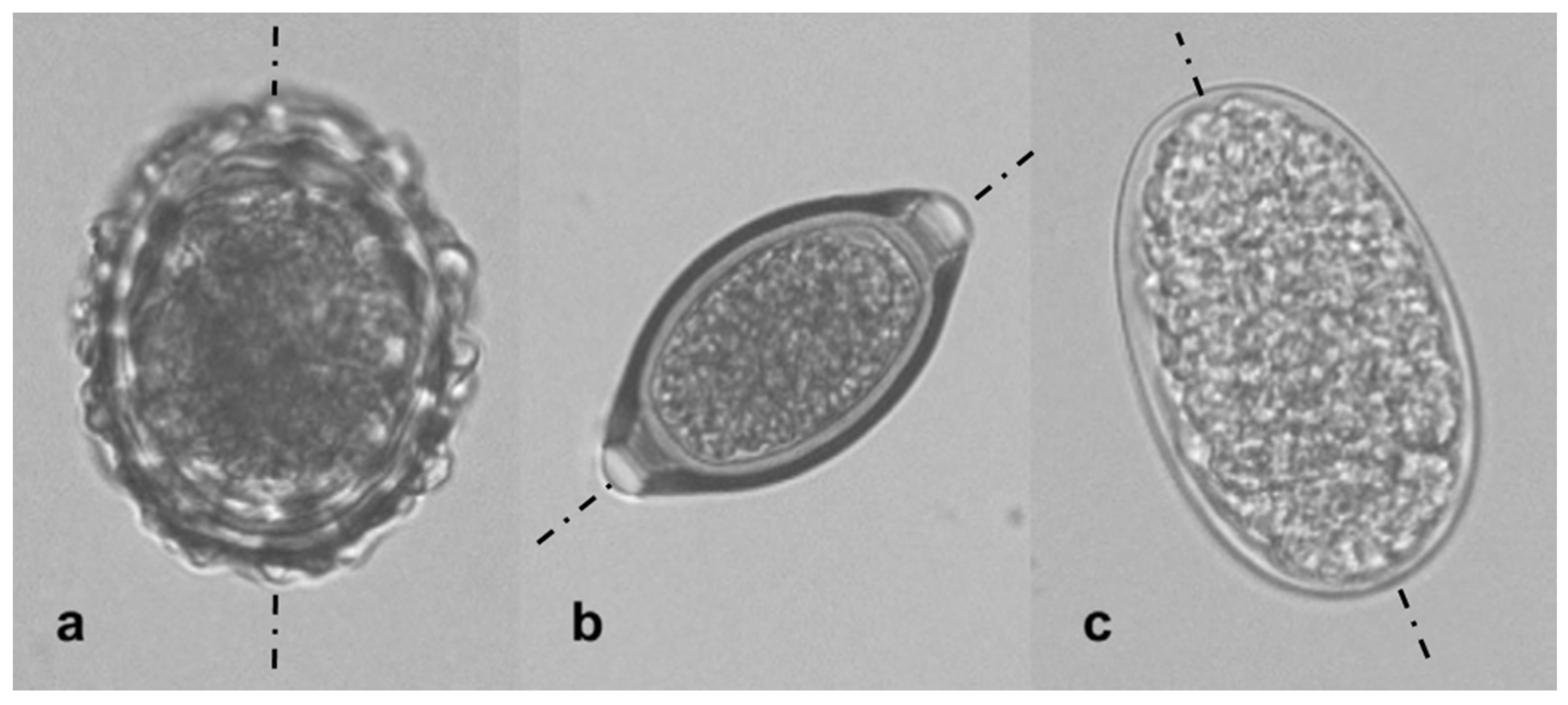
For each individual category of the parasites, suspensions of 500–600 eggs were used [20]. Obviously, the size and shape of the individual eggs showed a variation within each category. Typical morphologies of the eggs in each category are shown in Figure 1 (which is borrowed from Sengupta et al. [20], where the symmetry lines are added to the original figure).
Although there are many differences in the shapes of the eggs in detail, there are also common features at large. The shapes seem to exhibit an approximate rotational symmetry around an assumed symmetry axis and resemble the shape of an ellipsoid approximately. For a general characterization of the shapes, following Sengupta et al. [20], a length, L (as the extension of the egg along the symmetry line) and a width, W (perpendicular to the symmetry line) can be defined. An aspect ratio, a, can be defined as a = L/W. Sengupta et al. [20] assumed that a mean egg size can be characterized by a mean egg diameter (dA), that is the arithmetic average of the mean length (L) and mean width (W) as
The measured geometry parameters as well as the material densities of the eggs are presented in Table 2.
3. Theoretical Calculation of Sink Velocity
3.1. Stokes Law for Sphere
For a spherical shape with diameter d, the sink velocity () of a particle can be obtained after the Stokes theory as follows [22]
Equation (2) can be used to obtain an approximation for the sink velocity of the non-spherical eggs, using a representative diameter, such as (Equation (1)) for d in Equation (2).
3.2. Sink Velocity as Function of Drag Coefficient
For a spherical particle experiencing a drag force () in a fluid with density , the drag coefficient () can be defined as [19]
where and u denote the particle velocity and local fluid velocity, respectively (for simplicity, the vectorial character of the velocities are not additionally indicated in the equation). Based on the relative velocity, a particle Reynolds number can be defined as
where μ denotes the fluid viscosity.
For the limit of vanishingly small Reynolds numbers (Re << 1), the Stokes theory leads to the following expression for the drag coefficient for a sphere [19]
Oseen [23] provided a theoretical improvement of the Stokes theory for slightly larger Reynolds numbers (Re < 1), which led to the following expression [19]
Inspecting the results of Sengupta et al. [20], assuming a spherical shape with an assumed average diameter, one can see that the resulting particle Reynolds numbers (Equation (4)) are lower than 0.02, falling well in the range covered by the above expressions.
Assuming a uni-directional flow (with velocity u) for simplicity, the drag force () acting on a spherical particle with diameter can be expressed as . The gravity force () is given by (including buoyancy) . Assuming that only these forces are acting externally on the particle, the momentum balance of the particle can be expressed as , where is the inertia force with , the term representing the particle’s acceleration. The sink velocity is defined as the velocity of the particle in the special case of a non-accelerating particle motion () within quiescent water (u = 0). Substituting these conditions (, u = 0) in the particle momentum balance given above, the particle velocity as function of the drag coefficient can be obtained as
Thus, the sink velocity can be obtained via Equation (7) based on a known drag coefficient (that may differ from the above-mentioned theoretical expressions). This is the approach adopted in the present study, where drag coefficients are first calculated, and then the sink velocities are obtained from Equation (7). This approach has also the principal advantage that the derived drag coefficient expressions can also be used in a more general sense. The drag coefficient expressions can then be used not only for the sinking process in quiescent water, but also more generally, for the case of calculating egg motion in a flow field within the framework of a Eulerian–Lagrangian [24] or Eulerian–Eulerian [25] formulation, as encountered in different fields of application.
4. Characterization of Egg Shapes
For enabling a numerical investigation, the egg shapes need a mathematical characterization. As the eggs of the three different species exhibit quite different shapes (Figure 1), it is obvious that the shapes within a single category may also show variations in size. For the variations in L and W, Sengupta et al. [20] reported deviations in the range 4–8% and 7–13% from the average values, respectively, for all three egg categories. Presently, it is generally assumed that a single generic shape can be defined for each category, in terms of well-defined geometric forms, depending on L and W. In general, it is intended that the shape variations in a category can then be obtained by changing the parameters L and W accordingly. However, in the present study, no shape variations are attempted and constant values of L and W for each category are assumed (Table 2).
4.1. Oesophagostomum spp. (OES)
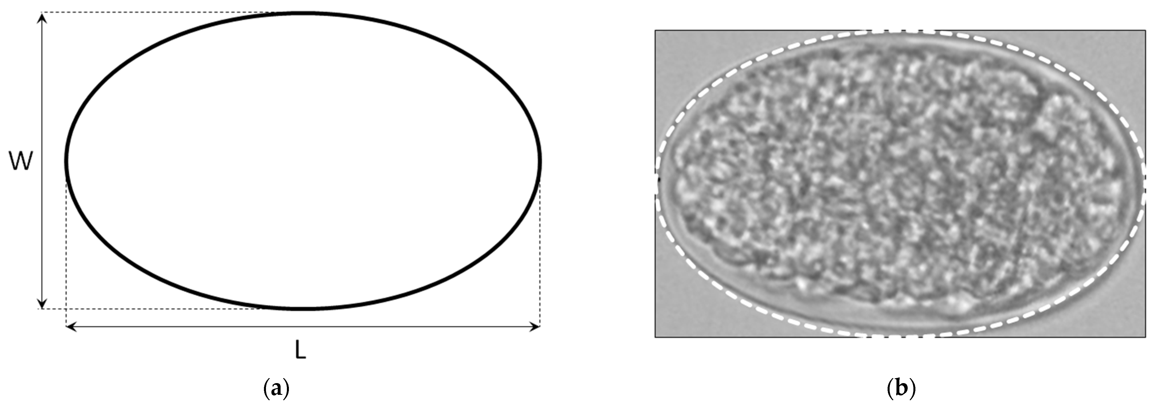
The shape of this egg is very similar to a perfect ellipsoid (Figure 1c). Thus, the shape’s contour in the plane cutting through the symmetry axis can be described by an ellipse with the height and width being L and W, respectively, as illustrated in Figure 2a. In Figure 2b, the ideal elliptic contour (dashed line) is compared with the real shape of the OES egg (Figure 1c). One can see that the agreement is quite good.
4.2. Trichuris suis (TRI)
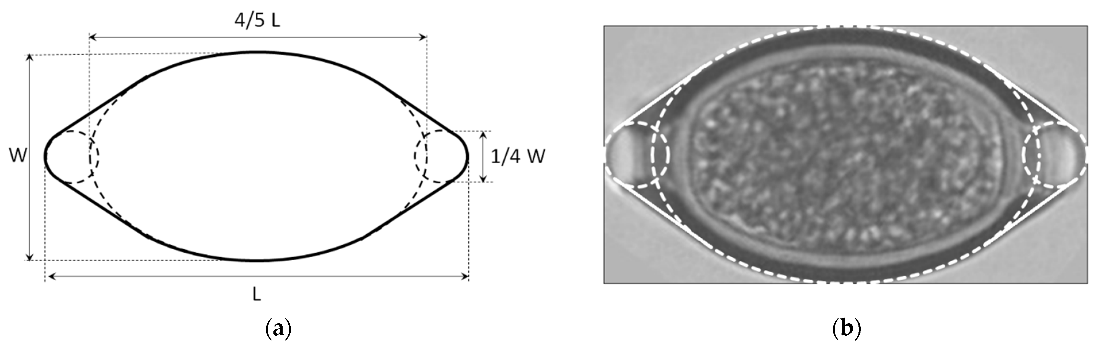
Inspecting the shape (Figure 1b), it seems that the two-dimensional contour of the axisymmetric body can be characterized with the help of a large ellipse in the core and two smaller circles on the edges, as sketched in Figure 3a, where the ellipse and circles are connected by straight tangents. Based on the image (Figure 1b), the height and width of the ellipse are assumed to be given by 4/5 L and W, respectively, whereas the diameter of the circles is assumed to be 1/4 W (Figure 3a). In Figure 3b, the assumed, idealized shape (dashed line) is compared with the real shape of the TRI egg (Figure 1b), where a good agreement can be observed.
4.3. Ascaris suum (ASC)
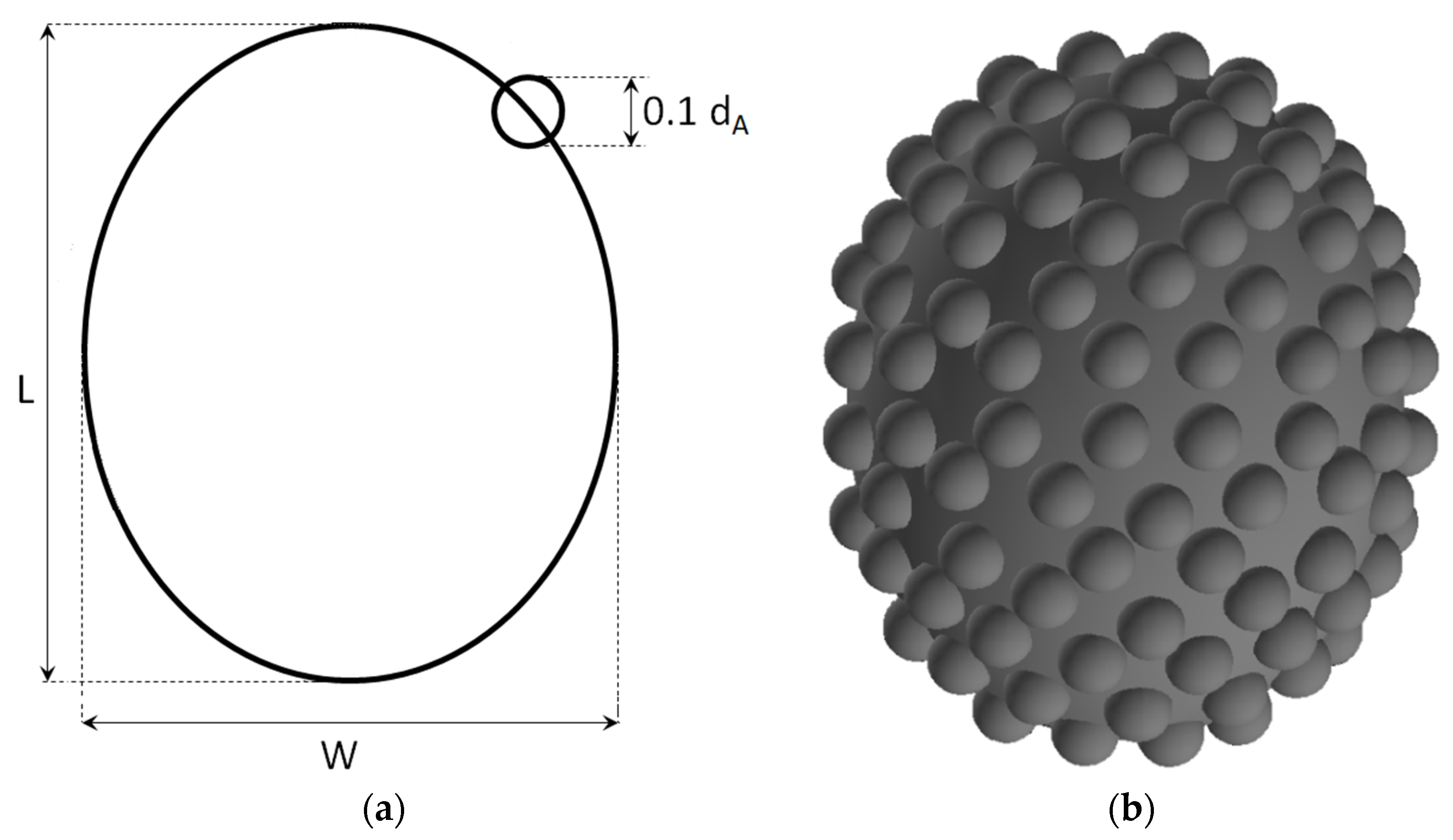
This shape is much more difficult to characterize, since it does not have a smooth surface, and the surface structure has an arbitrary (random) character. As an idealization, a basic ellipsoid shape can again be assumed, which is corrugated by nearly spherical structures at smaller scale. In the absence of more detailed data, inspecting the image provided by Sengupta et al. [20] (Figure 1a), it is assumed that the surface corrugations can be idealized, on average, as spheres with diameter 0.1 (Equation (2)), which are placed on the ellipsoidal surface in such a manner that their centers coincide with the surface, leading to the shape of a semi-sphere for each corrugation (Figure 4a).
Assuming this to be a reasonable idealization, a further difficulty lies in estimating the total number of corrugating spheres on the three-dimensional surface and their distribution. For estimating the number of corrugations, the following procedure is applied: First, based on the available image (Figure 1a), the number of corrugations (n) along the periphery of the visible silhouette (of the 2D section) is counted. Obviously, this count (n) is not necessarily exact, but as a result of a subjective visual impression, only indicative. Dividing the periphery of the silhouette by n, a curve length of Δ is obtained, which gives the length of the periphery associated with a corrugation, on the average (on a 2D section). For the 3D surface of the ellipsoid, it is then assumed that the partial surface occupied by a single spherical corrugation is given by a square with the size Δ × Δ, on average. Thus, the total number of spherical corrugations (N) distributed over the smooth 3D surface of the inner ellipsoid is obtained by dividing the total surface of the ellipsoid by an area of Δ × Δ. Here, the ellipsoidal surface of the egg is approximated by that of a sphere with equivalent diameter, which can be assumed to be reasonable, since the aspect ratio of this egg is rather low (Table 2). Based on this, the total number of corrugating spheres can be obtained as N = n2/π. In the present case with n = 23, N = 168 results. As already pointed out, corrugations have variable size, and they are distributed unevenly. It would be possible to imitate these natural patterns by introducing some randomness in the size and distribution of the corrugations. However, at the current stage, the corrugations are assumed to have a uniform size, as already mentioned before. Further, it is assumed that they are distributed rather regularly in a principally uniform pattern over the surface of the ellipsoid. The generated geometry according to these assumptions is presented in Figure 4b.
5. Mathematical Modelling and Numerical Solution
For the computational analysis, the general-purpose, finite volume method (FVM) based [26] computational fluid dynamics (CFD) code ANSYS Fluent 18.0 is used [27].
The continuity and Navier–Stokes equations for the incompressible flow of a fluid (water) with constant viscosity are solved. At the presently prevailing very low Reynolds numbers, the possibility transitional turbulence [28] can be excluded and the flow is assumed to remain always laminar. The study is performed in steady state, where the egg is stationary in the considered reference frame and blown by a given inflow velocity. The Reynolds number is defined based on the prescribed inlet velocity.
In the numerical formulation, the velocity–pressure coupling is treated by the so-called SIMPLEC procedure [29]. The convective terms are discretized by a second-order accurate upwinding scheme [30]. Within the iterative procedure, the under-relaxation factors used for the pressure and velocity are 1.0 and 0.5, respectively. For convergence, the threshold values for the scaled residuals are set to 10−9, which are 106 times smaller than the default value of 10−3.
6. Solution Domain, Boundaries, Validation
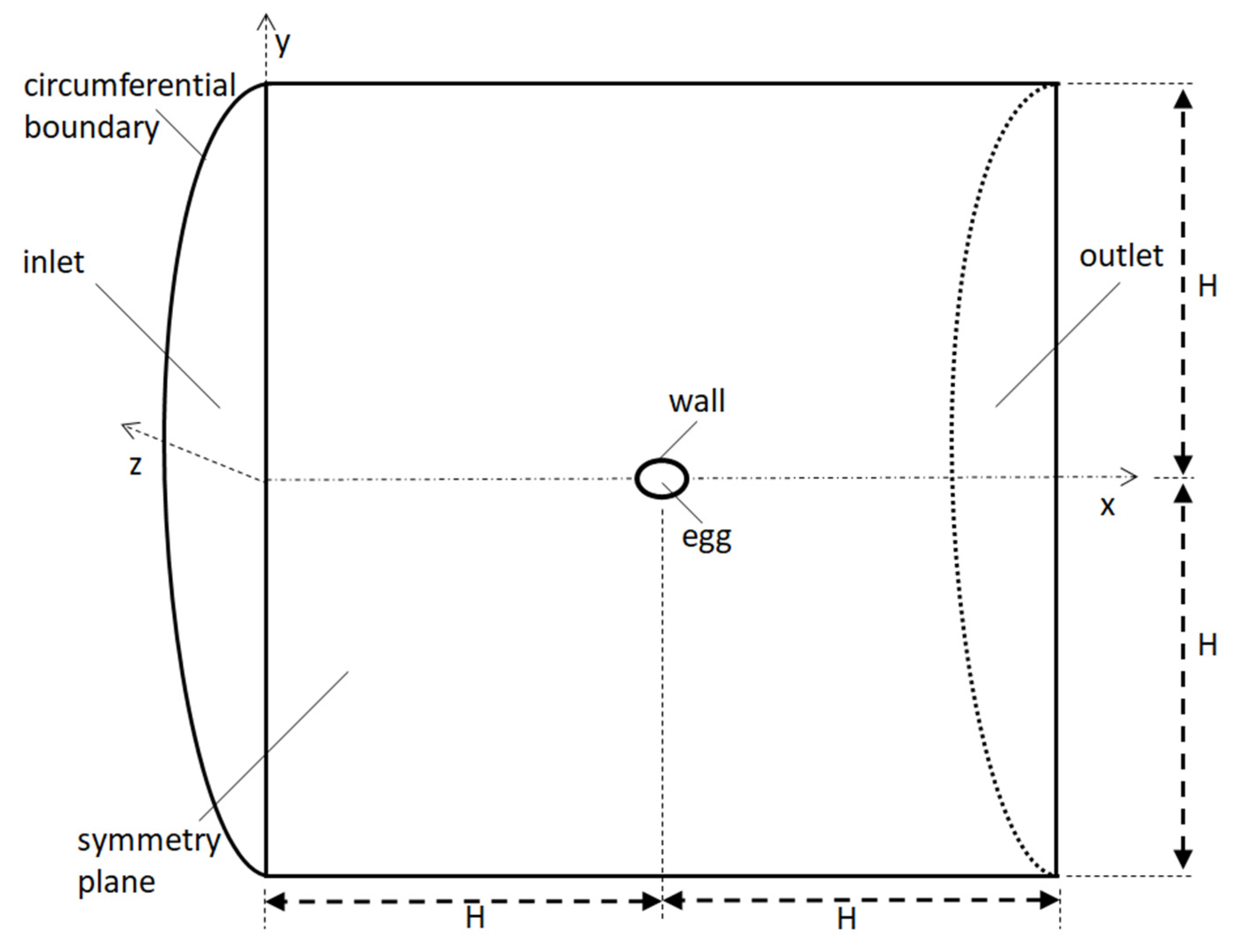
The solution domain is defined to have the shape of a cylinder with its height (2H) being equal to its diameter (2H), with the egg placed in the middle. All considered egg shapes (at least in the form they are presently idealized) have a symmetry axis and thus offer a symmetry plane. Aligning this plane with that of the cylindrical domain, the solution domain can be defined as half of the physical domain, i.e., as a half cylinder (containing the half of the egg) as depicted in Figure 5.
Obviously, the straight plane going through the middle of the cylinder (and of the egg) is defined as a symmetry plane (Figure 5). Thus, the inlet and outlet boundaries are semi-circles. At the inlet boundary the velocity components are prescribed as boundary condition, where a uni-directional flow with constant velocity is assumed. At the outlet boundary, the normal velocity gradients are assumed to be zero (fully developed flow) along with a prescribed constant static pressure. The circumferential surface enclosing the cylindrical domain is assumed to be an impermeable slip boundary with zero shear-stress. The surface of the egg is a wall, with the no-slip boundary condition.
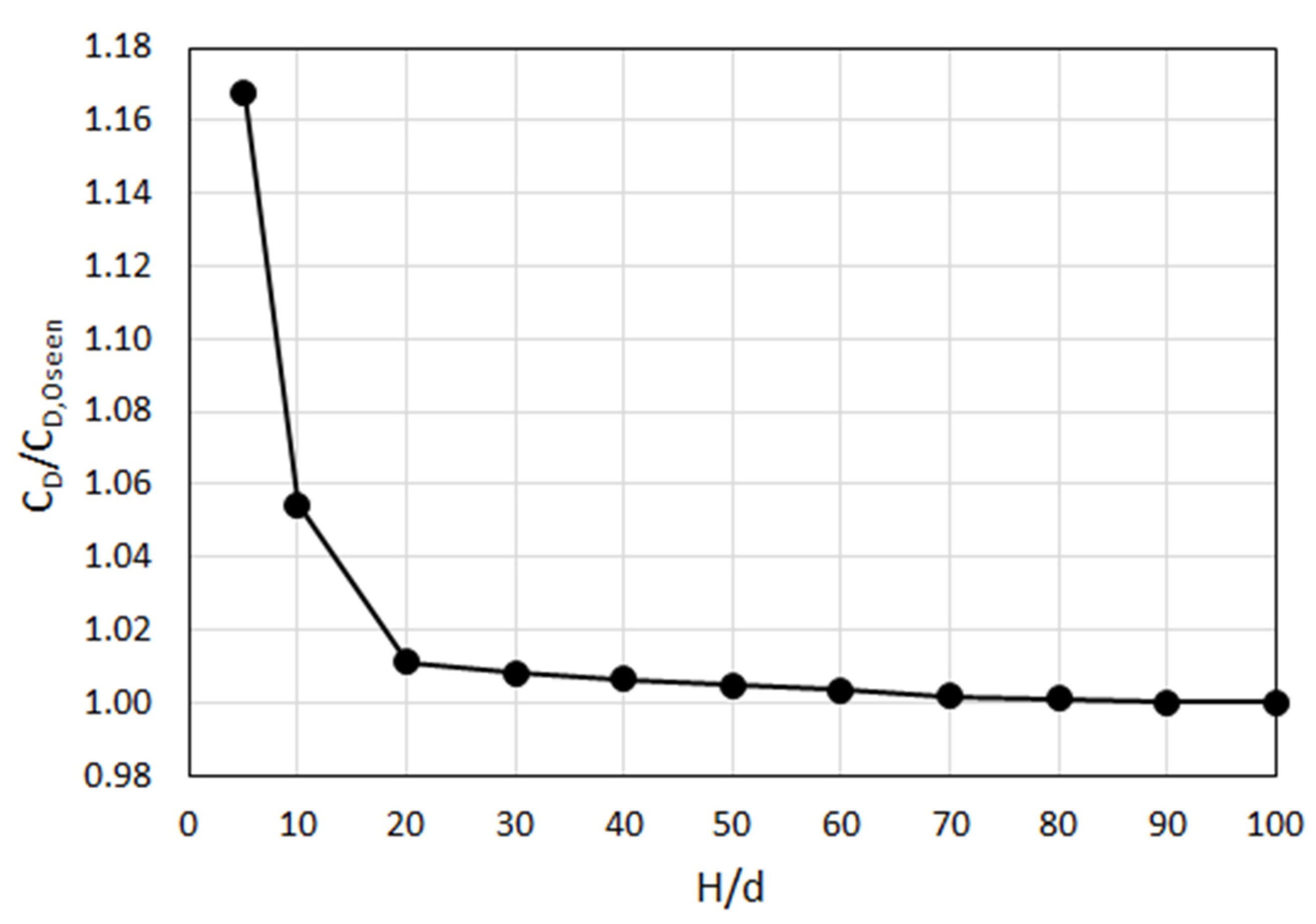
An important aspect with the definition of the solution domain is the definition of its size. The boundaries shall be sufficiently far from the object (the egg) so that the assumed boundary conditions have a negligible influence on the resulting flow field around the object. To determine the required extension of the domain, a series of calculations are performed with varying domain size (H, Figure 5). This is done for a quite low Reynolds number, i.e., for Re = 0.001 (since the “blockage effect” is stronger for low Re). Please note that these calculations are performed using grids, providing sufficient grid independence, which will be addressed in the next section. In the present calculations, to investigate the role of the domain size, a spherical egg shape with a diameter d is assumed.
The variation of the predicted drag coefficient () on the sphere, normalized by the theoretical expression by Oseen (, Equation (6)), with varying domain size is illustrated in Figure 6.
One can see in Figure 6 that a variation of the predicted drag coefficient is rather large for H/d < 20. For larger domains (H/d > 20), the drag coefficient is only mildly affected by the increasing size. Beyond H/d = 30, the relative change is less than 1% and the change beyond H/d = 80 is vanishingly small. This comparison with the theory can also be seen as a “validation” of the present numerical procedure, since the theoretical value of the drag coefficient by Oseen is very accurately predicted (for sufficiently large domain). For ensuring a sufficiently large domain in all considered cases, a domain size with H/d = 100 is used for all calculations.
7. Grid Generation
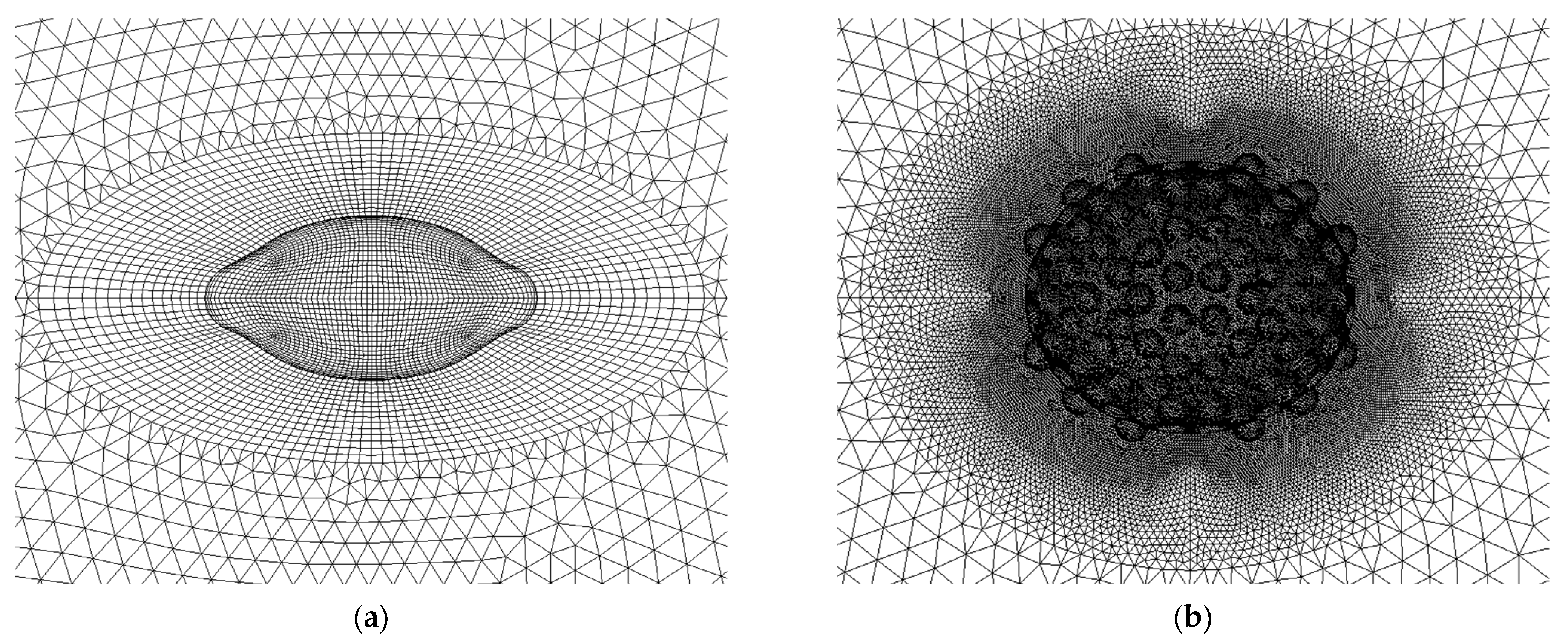
In generating the grid, the solution domain is divided into inner and outer regions. The inner region is defined by an ellipsoid around the egg, which is twice as large (2L × 2W). A bi-directionally equidistant surface grid is generated on the egg surface. In the inner ellipsoidal domain, in the third dimension, which is perpendicular to the egg surface, a rather mild grid expansion ratio (1.00–1.05) is used. A structured grid is used for OSC and TRI in the inner domain. For ASC, the surface corrugations require a finer grid resolution and make the application of a structured grid difficult. Thus, for ASC, the inner ellipsoid is discretized by a finer unstructured grid. In the outer domain, an unstructured discretization with tetrahedral cells is used, which expands with an expansion ratio of 1.1 towards the boundaries of the solution domain.
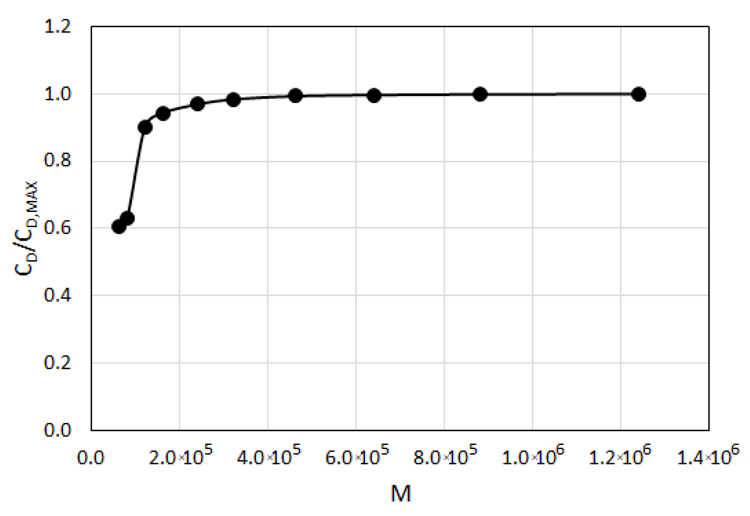
A careful grid independence study is performed by varying the grid resolution systematically, requiring constancy of the predicted drag coefficient (with deviation less than 0.5%). The grid independence study is exemplarily presented in Figure 7, for TRI, Re = 0.01, θ = 0°. In the figure, variation of predicted drag coefficient with number of cells (M) is displayed, where the drag coefficient, , for a grid is normalized by the by the maximum value of the drag coefficient, , obtained on the finest grid. One can see that variation of the drag coefficient is rather strong for M < 100,000 and becomes quite mild for M > 200,000, while a deviation less than 1% is observed for grids beyond M ≥ 400,000.
The generated grids for OES and TRI had about 640,000 cells, while the grids for ASC consisted about 2,200,000 cells. Detailed views of grids for TRI and ASC are illustrated in Figure 8.
8. Influence of Egg Orientation on Drag Force
For a spherical object shape, the flow direction does, obviously, not play a role in the drag coefficient. For non-spherical objects, like the presently considered eggs, the drag coefficient depends on the orientation of the object with respect to the flow direction. Since we are applying a steady-state analysis (in a relative frame), where a stationary egg is approached by a given velocity, a relative orientation of the egg with respect to flow needs to be pre-assumed for each calculation. In reality, the eggs can arbitrarily take any orientation to flow direction. For considering this effect, drag coefficients are calculated for different orientations of the eggs to the flow direction. Subsequently, their average value is assumed to be a representative drag coefficient, which takes this effect (varying relative orientation), on average, into account.
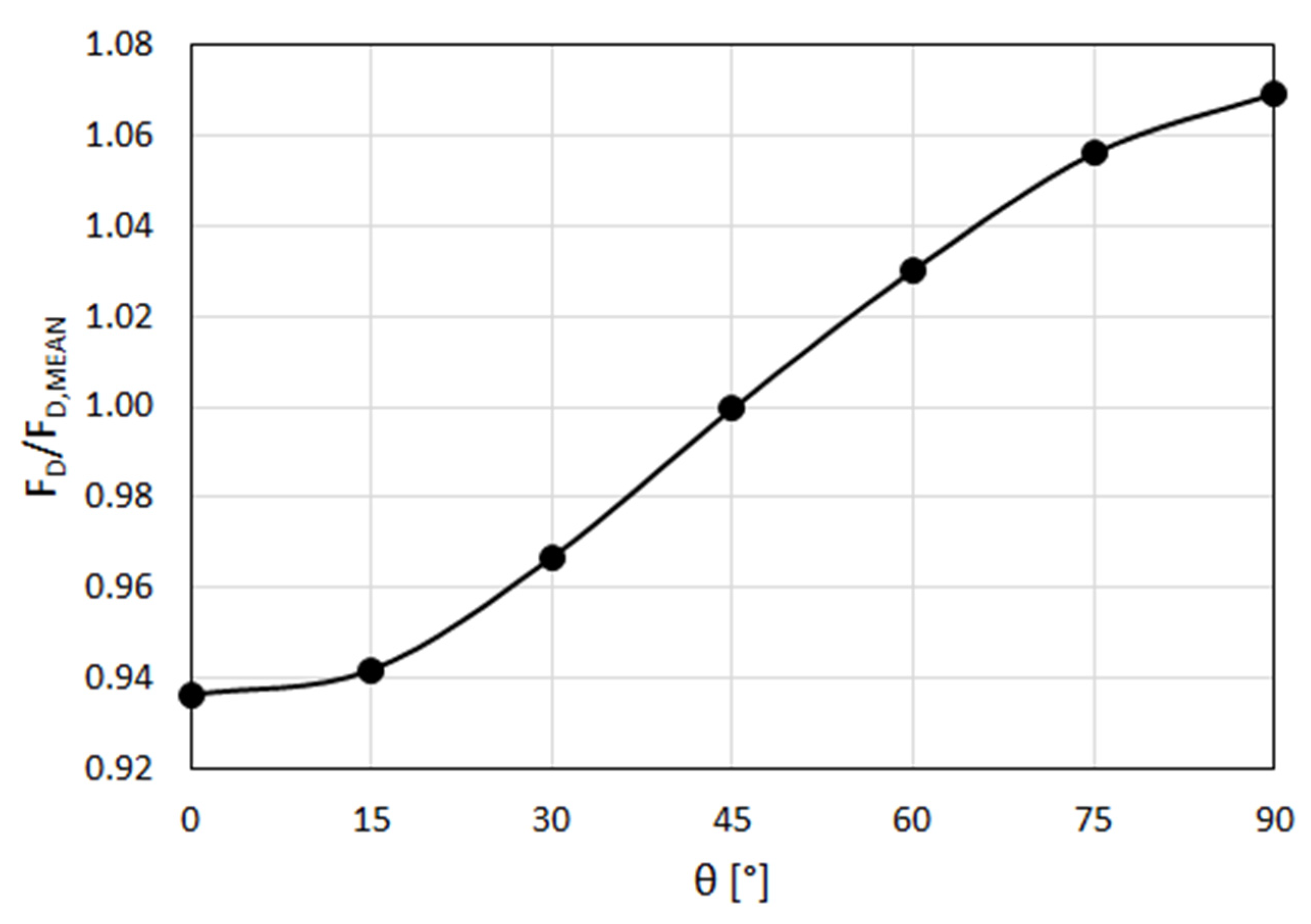
The variation of the drag force with the egg’s orientation to flow direction is expected to increase with aspect ratio. Among the considered egg shapes, the aspect ratio is the largest for TRI (Table 2). Thus, the effect of orientation is studied, first, for TRI. The “horizontal” egg position is the one, where the major axis (i.e., the length, L) of the ellipsoidal egg shape is aligned with the horizontal flow direction (x direction, Figure 5), where the angle (θ) between the L axis and flow direction is zero (θ = 0°). The “vertical” egg position is defined to be the one, where the L axis is perpendicular to the flow direction, corresponding to θ = 90°. Between the horizontal (θ = 0°) and vertical (θ = 90°) positions, five different orientations with θ = 15°, 30°, 45°, 60°, 75° are considered.
Variation of the calculated drag force (normalized by mean drag force) with orientation angle is presented in Figure 9, for TRI (FD,MEAN is the arithmetic average of the drag forces calculated for seven θ values). Practically the same curve is obtained for different Reynolds numbers within the range 0.0025 < Re < 1.
One can see that the drag coefficients for different orientations deviate from the mean value within a range of approximately ±7%, for TRI. This deviation is smaller for shapes with a smaller aspect ratio (Table 2), i.e., approximately ±4% for OES and approximately ±2% for ASC.
In this work, in determining the drag coefficients and sink velocities, the average drag forces used are obtained based on calculations for different orientations, as explained above.
9. Results
9.1. Flow Fields
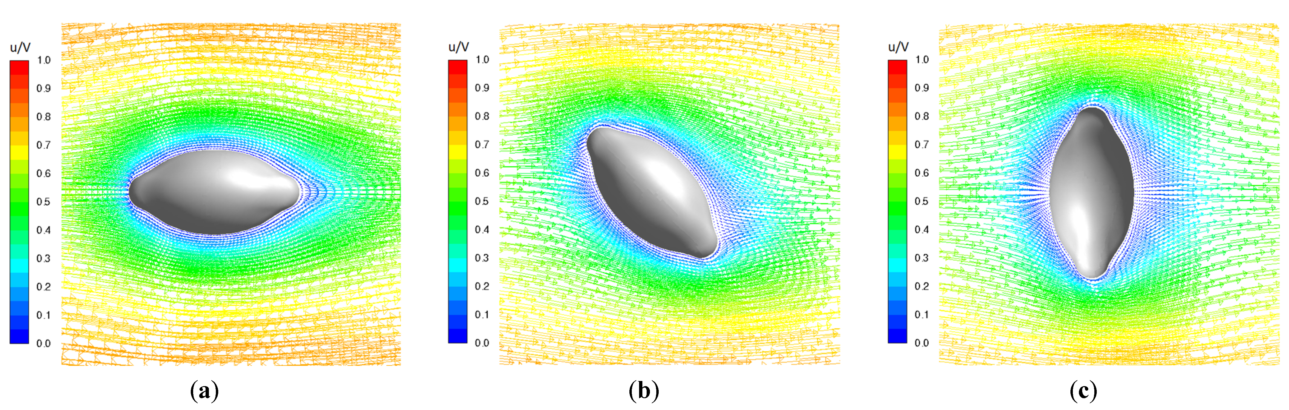
In this section, the distribution of flow variables for selected cases is presented. Figure 10 presents detailed views of the velocity vector field in the symmetry plane, for TRI, for three relative orientations of the egg (θ = 0°, 45°, 90°), for Re = 0.01. The velocity vector field distribution (scale is given for non-dimensionalized velocity u/V) around the egg shows different patterns in the downstream compared to upstream, manifesting a noticeable effect of the flow inertia, although the Reynolds number is quite low (Figure 10).
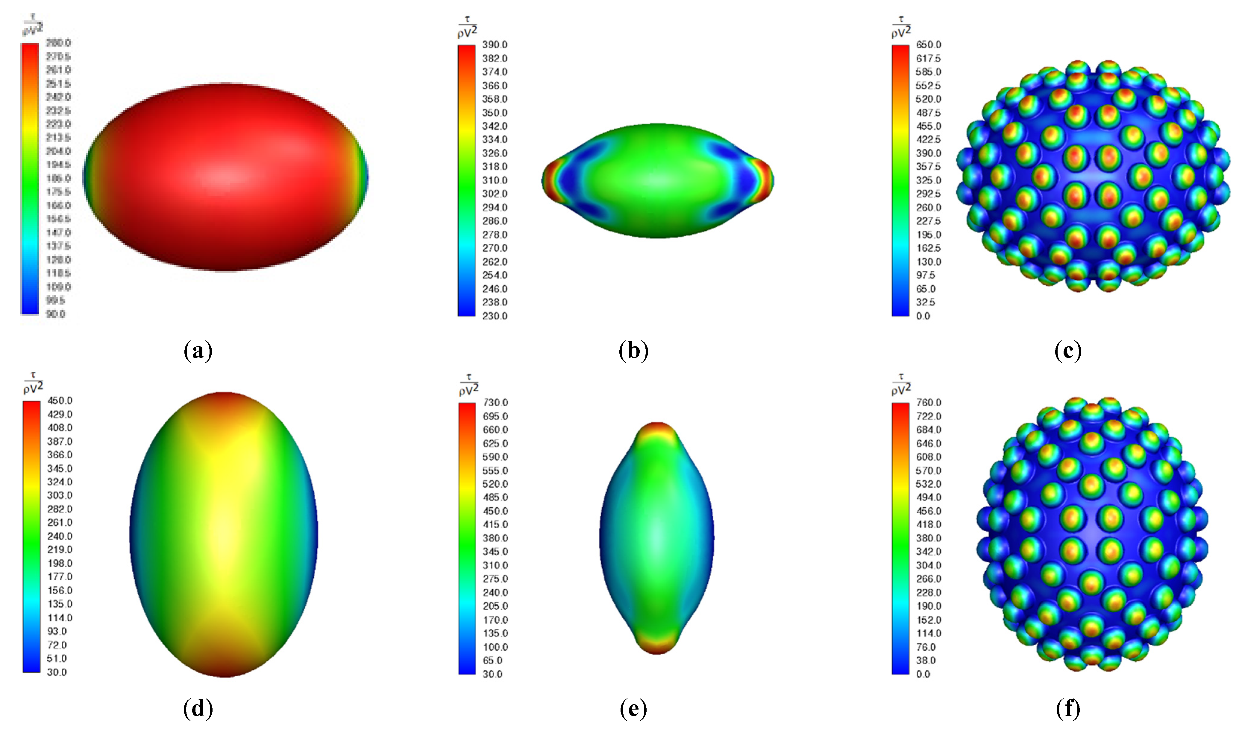
The shear stress distributions (non-dimensionalized by fluid density and inlet velocity, as ) over the egg surface, predicted for Re = 0.01, for OES, TRI, and ASC are presented for the horizontal (θ° = 0, upper raw) and vertical (θ° = 90, lower raw) relative positions of the eggs, as shown in Figure 11.
One can see that the maximum shear stress values occur at different positions depending on the shape. For ASC, it is interesting to note that the maximum shear stresses occur at the peaks of the spherical corrugations, whereas the base, ellipsoidal surface experiences a very low shear stress.
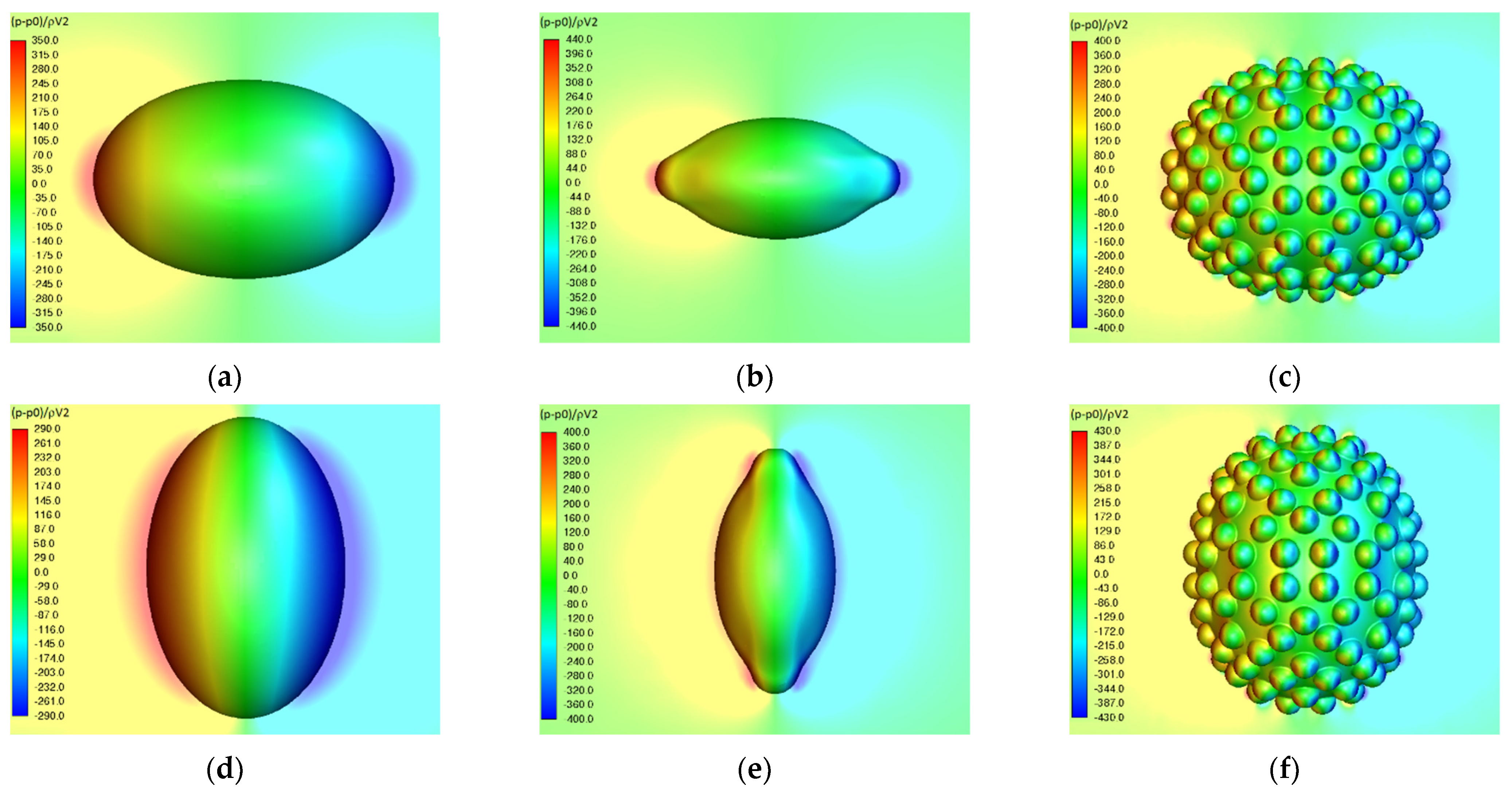
The non-dimensional relative pressure is defined as , where the reference pressure, , is the pressure in the far field downstream. The non-dimensional relative pressure distributions over the egg surface and in the symmetry plane in the egg’s nearfield, predicted for Re = 0.01, for OES, TRI, and ASC, are presented for the horizontal (θ° = 0, upper raw) and vertical (θ° = 90, lower raw) relative positions of the eggs, as shown in Figure 12.
9.2. Drag Coefficients
The predicted average drag coefficients (Section 8) are expressed as a correction of Oseen’s law (Equation (6)) as
where f is a correction factor, which applies a “shape specific” correction to the Oseen’s law for sphere.
The measured and expected sink velocities imply Reynolds numbers that are within the range 0.0025–0.02. Thus, for the present purpose of determining the sink velocities, the calculations are performed to cover this range by four Reynolds numbers, i.e., Re = 0.0025, 0.05, 0.1, 0.2. The calculated correction factors at these four points showed a rather weak Reynolds number dependence within the considered range. Still, for the sake of better accuracy, the Reynolds number dependence of the correction factor f is considered. This is done by a curve-fitting to the calculated values (with coefficient of determination R2 higher than 0.96), resulting in an expression in the form
The coefficients α and β obtained for different egg shapes are listed in Table 3.
9.3. Sink Velocities
Employing the predicted drag coefficients as functions of Reynolds number (Equations (6), (8), (9)), the sink velocities can be obtained from Equation (7). Since is a function of Reynolds number, and thus depends on the velocity, Equation (7) is non-linear in velocity and can only be solved iteratively to obtain the sink velocity. Thus, the egg-shape dependent sink velocities () are obtained by an iterative solution of Equation (7), using the predicted drag coefficients.
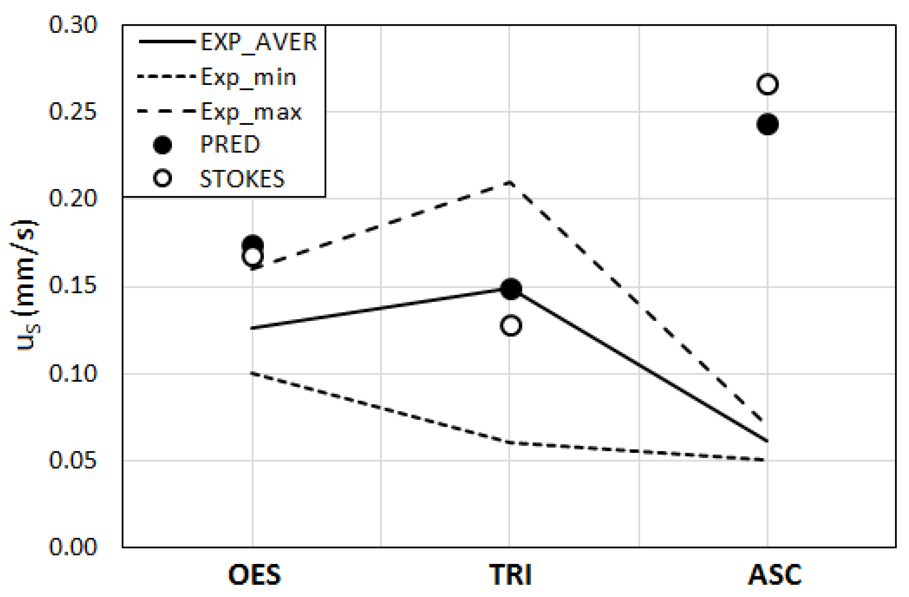
The predicted sink velocities are provided in Table 4. In the table, the experimentally obtained average sink velocities, as well as the sink velocities obtained by the Stokes theory are also presented.
The presently predicted sink velocities, as well as the measured ones, and the values provided by the Stokes law are displayed graphically in Figure 13. Since the experimentally obtained values showed a spread, the minimums and maximums of the experimentally obtained values are also indicated in the figure.
In Figure 13, one can observe that the presently predicted, shape-specific sink velocities do not very significantly differ from those calculated by the Stokes law.
For ASC, the Stokes law is over-predicting the experimental value strongly. The present calculations predict a lower sink velocity. This is, however, still too high compared to the experimental value. It is rather surprising to see that the predicted sink velocity for the real shape does not differ much from a sphere (Stokes law), especially for this egg. A much higher flow resistance, and consequently, a much lower sink velocity would be expected for this egg shape (ASC) due to its surface corrugations. It seems that the latter do not necessarily create a very high drag force. The predicted shear stress distributions shown in Figure 11c,f can be seen to provide an explanation for this behavior. The corrugations seem to “protect” the ellipsoidal base surface against large shear stresses, by “lifting” the boundary layer. High shear stresses occur only on the tips of the corrugations, whereas the lower surfaces are in contact only with lower velocities, and thus experience lower shear stresses. In a way, this resembles the so-called “shark skin” effect.
For TRI, a very good, a nearly perfect agreement of the present predictions with the measurements is observed. For this egg shape, the Stokes theory is showing an under-prediction, which is, however, not too far from the experimental value, compared to ASC.
For OES, the present predictions and the Stokes theory do not agree very well with the experiments and over-predict the measured value. This is also a rather unexpected behavior. Compared to the other egg shapes, the shape of this egg is less complicated and more similar to a smooth sphere. Thus, a better prediction would be expected, even by the Stokes law. The computationally predicted sink velocity is also not better than that of the Stokes theory, even slightly worse, with a slightly higher over-prediction. This may be seen to imply that the shape of an individual egg does not primarily determine the resulting sink velocity, but interactions and flocculation effects, which may indirectly depend on the surface shape and texture, are primarily influential in the resulting average sink velocity. The large discrepancy between the prediction and measurement observed for ASC seems to imply the same. The surface modelling of ASC was quite approximate and arbitrary. However, since the discrepancy between the prediction and measurement is very large, the details of the surface modelling do not seem to provide a sufficient explanation.
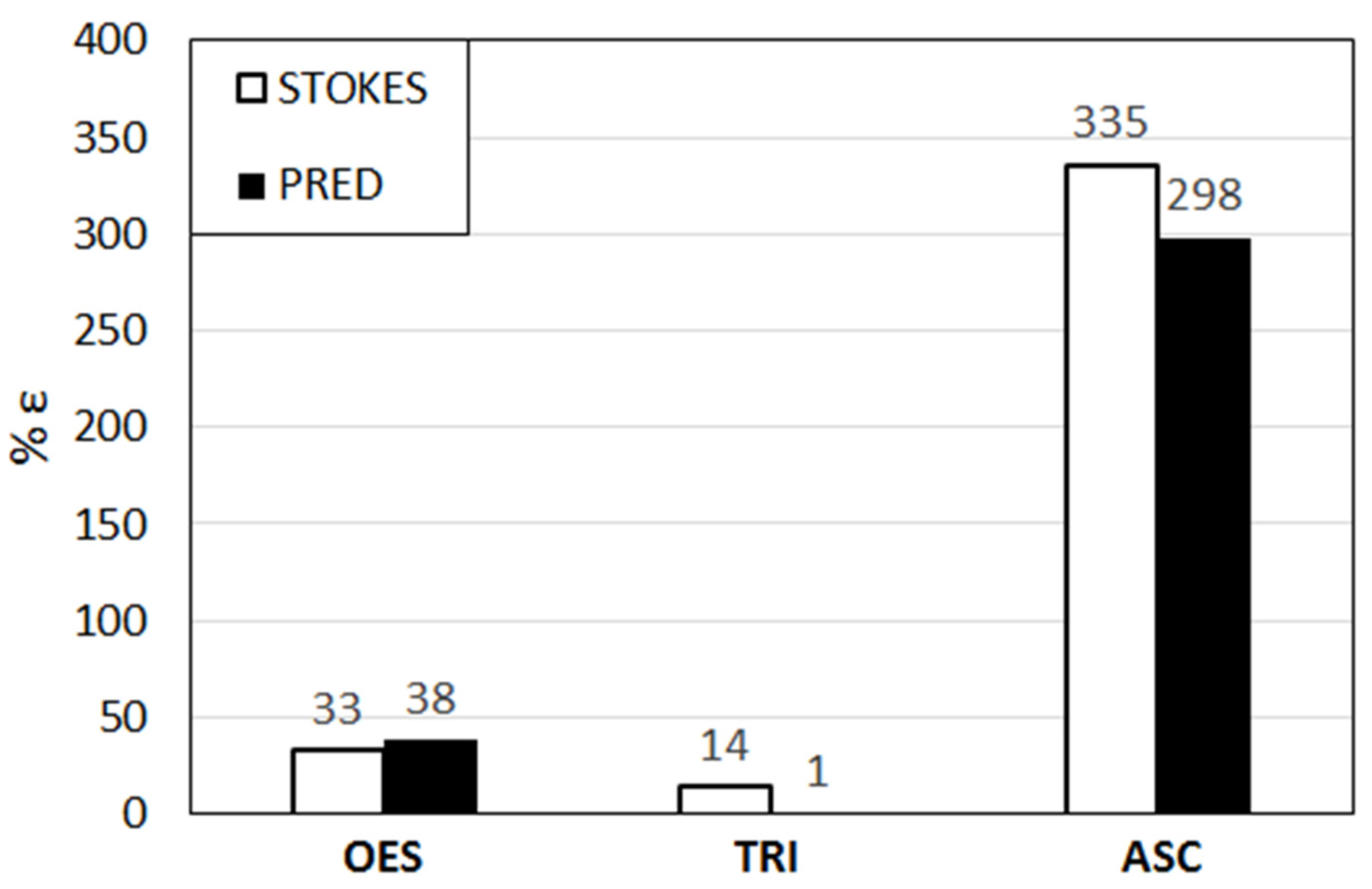
The percentage errors in the calculation of the sink velocity by the present predictions and by the Stokes law, with respect to the measured average sink values of Sengupta et al. [20], are presented in Figure 14 ().
The largest and smallest errors are observed for ASC and TRI, respectively. For ASC, the present predictions provide an improvement compared to the Stokes law, which is still far from being satisfactory. For TRI, the Stokes law provides a rather good agreement with the measurement. The present calculations lead to an even better prediction and agree nearly perfectly with the experimentally obtained average value. For OES a moderate agreement of the present prediction and the Stokes law with the measurement is observed. Here, the agreement of the Stokes law with the experimentally obtained average value is slightly better than the calculated one.
10. Conclusions
The sink velocities of helminth eggs of three types, namely Ascaris suum (ASC), Trichuris suis (TRI), and Oesophagostomum spp. (OES), in clean tap water are computationally determined by means of computational fluid dynamics. Results are compared with the experimentally obtained average sink velocities of Sengupta et al. [20], and the sink velocities delivered by the Stokes law. A main focus of the investigation has been to achieve a realistic modelling of the egg shape as accurately as possible, and thus to achieve an improvement against the Stokes theory that assumes a spherical shape.
Principally, an improvement is obtained for ASC and TRI. However, the overall predictive performance is not very satisfactory. For ASC, the over-prediction seems to be too large to be explained by eventual inaccuracies in the surface texture modelling. Although TRI has a shape, which is more complicated and deviates more from a sphere compared to OES, a better prediction is obtained for TRI than for OES. Such results imply that the detailed shape of an individual egg is not decisive for the resulting average sink velocity. Since populations of eggs, not individual eggs, were used in the experiments, interactions and flocculation effects (although clean tap water was used) might have played a more important role.
A further aspect is that the eggs might not be following straight, but more complex paths as they sink, with lateral and spinning movements that might have affected the overall sink behavior. This could not be considered precisely in the present modeling framework, although the orientation changes were considered on average, approximately.
Another point to consider is the fact that the measured average sink velocity is not necessarily a “physical”, but a “hypothetical” quantity, as it results from the arithmetic average of the really occurring values, which demonstrated a certain scatter. For the measured sink velocities, the standard deviations from the mean were about 9%, 41%, and 18%, for ASC, TRI, and OSE, respectively. Similarly, variations were observed in the shapes of the eggs. For the measured L, the standard deviations from the mean were about 8%, 4%, and 7% for ASC, TRI, and OES, respectively, whereas these numbers were 7%, 9%, and 14% for W, while the aspect ratio (a) showed a deviation of about 10% from the mean for all egg types. It is not necessarily clear how well the presently assumed average egg sizes and shapes correlate with the experimentally obtained average sink velocities.
The present results show that a detailed analysis of the shapes of isolated eggs is not sufficient for an accurate computational prediction of the sink velocities of helminths eggs in water. For improvement, additional work with more sophisticated approaches, combined with a more detailed analysis of the experimental results, seems to be necessary.
Funding
This research was partially funded by the German Federal Environmental Foundation (Deutsche Bundesstiftung Umwelt, DBU) [34847/01-23].
Institutional Review Board Statement
Not applicable.
Informed Consent Statement
Not applicable.
Data Availability Statement
Presented data may be made available upon request from author.
Acknowledgments
The author would like to acknowledge the German Federal Environmental Foundation (Deutsche Bundesstiftung Umwelt, DBU), Osnabrück, Germany, for the funding support of this research project [Project number: 34847/01–23]. In particular, the continuous encouragement and support by Alexander Bonde and Franz-Peter Heidenreich are gratefully acknowledged.
Conflicts of Interest
The authors declare no conflict of interest.
Nomenclature
| a | Aspect ratio |
| Drag coefficient [-] | |
| d | Diameter [m] |
| Mean egg diameter [μm] | |
| f | Correction function [-] |
| Drag force [N] | |
| Gravity force [N] | |
| Inertial force [N] | |
| g | Gravitational acceleration [m s−2] |
| H | Radius and half-height of cylindrical solution domain [m] |
| L | Length [μm] |
| M | Number of computational cells [-] |
| p | Pressure [Pa] |
| Reference pressure [Pa] | |
| Particle Reynolds number [-] | |
| t | Time [s] |
| u | Flow velocity [m s−1] |
| Particle/egg velocity [m s−1] | |
| Sink velocity [m s−1] | |
| V | Inlet velocity |
| W | Width [μm] |
| x,y,z | Cartesian coordinates [m] |
| Greek symbols | |
| α | Coefficient of correction function [-] |
| β | Coefficient of correction function [-] |
| θ | Angle between egg symmetry axis and flow direction [°] |
| μ | Molecular viscosity of water [Pa s] |
| Density of water [kg m−3] | |
| Density of particle/egg [kg m−3] | |
| τ | Shear stress [Pa] |
| %ε | Percentage error between experiments and predictions or Stokes law [-] |
| Subscripts | |
| MAX | Maximum value |
| MEAN | Mean value |
Abbreviations
| ASC | Ascaris suum |
| CFD | Computational Fluid Dynamics |
| EXP | Experimental |
| EXP_AVER | Experimental average value |
| Exp_max | Experimental maximum value |
| Exp_min | Experimenral minimum value |
| OES | Oesophagostomum spp. |
| OSEEN | Value obtained from Oseen law |
| PRED | Predicted |
| PRED/STOKES | Predicted value, or value obtained from Stokes law |
| STOKES | Value obtained from Stokes law |
| TRI | Trichuris suis |
| WSP | Waste Stabilization Ponds |
| WHO | World Health Organization |
References
- Cirelli, G.L.; Consoli, S.; Licciardello, F.; Aiello, R.; Giuffrida, F.; Leonardi, C. Treated municipal wastewater reuse in vegetable production. Agric. Water Manag. 2012, 104, 163–170. [Google Scholar] [CrossRef]
- Zhang, Q.; Achal, V.; Xu, Y.; Xiang, W.-N. Aquaculture wastewater quality improvement by water spinach (Ipomoea aquatic Forsskal) floating bed and ecological benefit assessment in ecological agriculture district. Aquac. Eng. 2014, 60, 48–55. [Google Scholar] [CrossRef]
- Lonigro, A.; Rubino, P.; Lacasella, V.; Montemurro, N. Faecal pollution on vegetables and soil drip irrigated with treated municipal wastewaters. Agric. Water Manag. 2016, 174, 66–73. [Google Scholar] [CrossRef]
- Fuhrimann, S.; Nauta, M.; Pham-Duc, P.; Tram, N.T.; Nguyen-Viet, H.; Utzinger, J.; Cisse, G.; Winkler, M.S. Disease burden to gastrointensinal infections among people living along the major wastewater system in Hanoi, Vietnam. Adv. Water Resour. 2017, 108, 439–449. [Google Scholar] [CrossRef] [Green Version]
- Gyawali, P.; Ahmed, W.; Sidhu, J.P.; Jagals, P.; Toze, S. Quantification of hookworm ova from wastewater matrices using quantitative PCR. J. Environ. Sci. 2017, 57, 231–237. [Google Scholar] [CrossRef] [PubMed]
- Cui, B.; Luo, J.; Jin, D.; Jin, B.; Zhuang, X.; Nai, Z. Investigating the bacterial community and ameobae population in rural domestic wastewater reclamation for irrigation. J. Environ. Sci. 2018, 70, 97–105. [Google Scholar] [CrossRef] [PubMed]
- Lepine, C.; Christianson, L.; McIsaac, G.; Summerfelt, S. Denitrfyning bioreactor inflow manifold design for treatment of aquacultural wastewater. Aquac. Eng. 2020, 88, 102036. [Google Scholar] [CrossRef]
- Guadie, A.; Yesigat, A.; Gatew, S.; Worku, A.; Liu, W.; Minale, M.; Wang, A. Effluent quality and reuse potential of urban wastewater treated with aerobic-anoxic system: A practical illustration for environmental contamination and human health risk assessment. J. Water Process. Eng. 2021, 40, 101891. [Google Scholar] [CrossRef]
- Kirby, R.M.; Bartram, J.; Carr, R. Water in food production and processing: Quantity and quality concerns. Food Control 2003, 14, 283–299. [Google Scholar] [CrossRef]
- Wang, C.; Parlange, J.-Y.; Schneider, R.L.; Rasmussen, E.W.; Wang, X.; Chen, M.; Dahlke, H.E.; Truhlar, A.M.; Walter, M.T. Release of Escherichia coli under raindrop impact: The role of clay. Adv. Water Resour. 2018, 111, 1–5. [Google Scholar] [CrossRef] [Green Version]
- Kamizoulis, G. Setting health based targets for water reuse (in agriculture). Desalination 2008, 218, 154–163. [Google Scholar] [CrossRef]
- Mara, D.; Sleigh, A. Estimation of Ascaris infection risks in children under 15 from the consumption of wastewater irrigated carrots. J. Water Health 2010, 8, 35–38. [Google Scholar] [CrossRef]
- WHO. Guidelines for the safe use of wastewater, excreta and greywater. In Wastewater Use in Agriculture; World Health Organization: Geneva, Switzerland, 2006; Volume 2. [Google Scholar]
- Yin, F.; Li, Z.; Wang, D.; Ohlsen, T.; Dong, H. Performance of thermal pretreatment and mesophilic fermentation system on pathogen inactivation and biogas production of faecal sludge: Initial laboratory sludge. Biosyst. Eng. 2016, 151, 171–177. [Google Scholar] [CrossRef]
- Ellis, K.V.; Rodrigues, P.C.C.; Gomez, C.L. Parasite ova and cysts in waste stabilization ponds. Water Res. 1993, 27, 1455–1460. [Google Scholar] [CrossRef]
- Stott, R.; May, E.; Mara, D.D. Parasite removal by natural wastewater treatment systems: Performance of waste stabilization ponds and constructed wetlands. Water Sci. Technol. 2003, 48, 97–104. [Google Scholar] [CrossRef] [PubMed]
- Ayres, R.M.; Alabaster, G.P.; Mara, D.D.; Lee, D.L. A design equation for human intestinal nematode egg removal in waste stabilization ponds. Water Res. 1992, 26, 863–865. [Google Scholar] [CrossRef]
- Chancelier, J.P.; Chebbo, G.; Lucas-Aiguier, E. Estimation of settling velocities. Water Res. 1998, 32, 3461–3471. [Google Scholar] [CrossRef]
- Schlichting, H. Boundary Layer Theory, 6th ed.; McGraw-Hill: New York, NY, USA, 1968. [Google Scholar]
- Sengupta, M.E.; Thamsborg, S.M.; Andersen, T.J.; Olsen, A.; Dalsgaard, A. Sedimentation of helminth eggs in water. Water Res. 2011, 45, 4651–4660. [Google Scholar] [CrossRef]
- Owen, M.W. Determination of the Settling Velocities of Cohesive Muds, Report No IT 161; Hydraulics Research Station: Wallingford, UK, 1976. [Google Scholar]
- Stokes, G.G. On the effect of the internal friction of fluids on the motion of pendulums. Trans. Cambr. Phil. Soc. 1851, Pt. II, 8–106. [Google Scholar]
- Oseen, C.W. Über die Stokessche Formel und über die verwandte Aufgabe in der Hydrodynamik. Ark. Math. Astron. Och Fys. 1910, 6, 1–20. [Google Scholar]
- Benim, A.C.; Stegelitz, P.; Epple, B. Simulation of the two-phase flow in a laboratory coal pulveriser. Forsch. Ing.-Eng. Res. 2005, 69, 197–204. [Google Scholar] [CrossRef]
- Benim, A.C.; Epple, B.; Krohmer, B. Modelling of pulverised coal combustion by a Eulerian-Eulerian two-phase flow formulation. Prog. Comput. Fluid Dyn. Int. J. 2005, 5, 345–361. [Google Scholar] [CrossRef]
- Moukalled, F.; Mangani, L.; Darwish, M. The Finite Volume Method in Computational Fluid Dynamics; Springer: Berlin, Germany, 2016. [Google Scholar]
- ANSYS Fluent Theory Guide; Release 18.0; ANSYS Inc.: Canonsburg, PA, USA, 2018.
- Bhattacharyya, S.; Chattopadhyay, H.; Benim, A.C. Computational investigation of heat transfer enhancement by alternating inclined ribs in tubular heat exchanger. Prog. Comput. Fluid Dyn. Int. J. 2017, 17, 390–396. [Google Scholar] [CrossRef]
- Van Doormal, J.P.; Raithby, G.D. Enhancements of the simple method for predicting incompressible fluid flows. Numer. Heat Transf. 1984, 7, 147–163. [Google Scholar] [CrossRef]
- Barth, T.J.; Jespersen, D.C. The design and application of upwind schemes on unstructured meshes. AIAA Paper No. 89-0366. In Proceedings of the 27th AIAA Aerospace Sciences Meeting and Exhibit, Reno, NV, USA, 9–12 January 1989. [Google Scholar]
Figure 1.
Morphology of the three helminth eggs considered (figure borrowed from Sengupta et al. [20], symmetry lines are added to original figure), (a) Ascaris suum (ASC), (b) Trichuris suis (TRI), (c) Oesophagostomum spp. (OES).
Figure 1.
Morphology of the three helminth eggs considered (figure borrowed from Sengupta et al. [20], symmetry lines are added to original figure), (a) Ascaris suum (ASC), (b) Trichuris suis (TRI), (c) Oesophagostomum spp. (OES).

Figure 2.
OES, (a) idealized elliptic shape, (b) idealized shape compared with real shape.

Figure 3.
TRI, (a) idealized shape, (b) idealized shape compared with real shape.

Figure 4.
ASC, (a) idealization of the shape, (b) modelled idealized shape.

Figure 5.
Sketch of solution domain.

Figure 6.
Variation of normalized drag coefficient with domain size for sphere with diameter d, for Re = 0.001 (achievement of the value of unity verifies the approach by manifesting its agreement with the Oseen theory).
Figure 6.
Variation of normalized drag coefficient with domain size for sphere with diameter d, for Re = 0.001 (achievement of the value of unity verifies the approach by manifesting its agreement with the Oseen theory).

Figure 7.
Variation of normalized drag coefficient with number of cells (TRI, Re = 0.01, θ° = 0).

Figure 8.
Detail views of computational grid, (a) TRI, (b) ASC (mesh in the symmetry plane is displayed, together with the mesh on the egg’s surface).
Figure 8.
Detail views of computational grid, (a) TRI, (b) ASC (mesh in the symmetry plane is displayed, together with the mesh on the egg’s surface).

Figure 9.
Variation of drag force with varying relative orientation (TRI).

Figure 10.
Velocity vector fields around TRI, for Re = 0.01, (a) θ = 0°, (b) θ = 45°, (c) θ = 90°.

Figure 11.
Dimensionless shear stress distribution over egg surface, for Re = 0.01, (a) OES, θ = 0°, (b) TRI, θ° = 0, (c) ASC, θ = 0°, (d) OES, θ = 90°, (e) TRI, θ° = 90, (f) ASC, θ = 90°.
Figure 11.
Dimensionless shear stress distribution over egg surface, for Re = 0.01, (a) OES, θ = 0°, (b) TRI, θ° = 0, (c) ASC, θ = 0°, (d) OES, θ = 90°, (e) TRI, θ° = 90, (f) ASC, θ = 90°.

Figure 12.
Dimensionless relative pressure distribution over the egg surface and in the symmetry plane in egg’s nearfield, for Re = 0.01, (a) OES, θ = 0°, (b) TRI, θ° = 0, (c) ASC, θ = 0°, (d) OES, θ = 90°, (e) TRI, θ° = 90, (f) ASC, θ = 90°.
Figure 12.
Dimensionless relative pressure distribution over the egg surface and in the symmetry plane in egg’s nearfield, for Re = 0.01, (a) OES, θ = 0°, (b) TRI, θ° = 0, (c) ASC, θ = 0°, (d) OES, θ = 90°, (e) TRI, θ° = 90, (f) ASC, θ = 90°.

Figure 13.
Presently predicted (PRED), experimental (EXP) and by the Stokes law (STOKES) provided sink velocities (), for the three egg types, OES, TRI and ASC. Minimum (Exp_min) and maximum (Exp_max) values obtained in the experiments [20] are also shown.
Figure 13.
Presently predicted (PRED), experimental (EXP) and by the Stokes law (STOKES) provided sink velocities (), for the three egg types, OES, TRI and ASC. Minimum (Exp_min) and maximum (Exp_max) values obtained in the experiments [20] are also shown.

Figure 14.
Percentage errors (%ε) in calculation of sink velocity, according to the present predictions (PRED) and based on the Stokes law (STOKES). Errors are calculated with respect to the experimental values.
Figure 14.
Percentage errors (%ε) in calculation of sink velocity, according to the present predictions (PRED) and based on the Stokes law (STOKES). Errors are calculated with respect to the experimental values.


Table 1.
Material properties of tap water [20].
Table 1.
Material properties of tap water [20].
| Density [kg m−3] | Viscosity [Pa s] |
|---|---|
| 997.8 | 0.00094 |
Table 2.
Geometry parameters and densities of helminth eggs [20].
Table 2.
Geometry parameters and densities of helminth eggs [20].
| Shape Parameters | Density [kg m−3] | ||||
|---|---|---|---|---|---|
| L [μm] | W [μm] | a [-] | dA [μm] | ||
| ASC | 67.20 | 55.41 | 1.22 | 61.31 | 1120 |
| TRI | 62.16 | 30.78 | 2.03 | 46.47 | 1100 |
| OES | 76.17 | 50.33 | 1.53 | 63.25 | 1070 |
Table 3.
Coefficients of correction function, Equation (9), for 0.0025 < Re < 0.02.
| α | β | |
|---|---|---|
| OES | 0.9606 | −0.1141 |
| TRI | 0.8559 | −0.1615 |
| ASC | 1.0936 | −0.1430 |
Table 4.
Sink velocities: predicted, experimental [20], Stokes law.
Table 4.
Sink velocities: predicted, experimental [20], Stokes law.
| Predicted | Experimental | Stokes Law | |
|---|---|---|---|
| OES | 0.1741 | 0.1262 | 0.1675 |
| TRI | 0.1495 | 0.1487 | 0.1280 |
| ASC | 0.2433 | 0.0612 | 0.2663 |
Publisher’s Note: MDPI stays neutral with regard to jurisdictional claims in published maps and institutional affiliations. |
© 2021 by the author. Licensee MDPI, Basel, Switzerland. This article is an open access article distributed under the terms and conditions of the Creative Commons Attribution (CC BY) license (https://creativecommons.org/licenses/by/4.0/).
Share and Cite
MDPI and ACS Style
Benim, A.C. Numerical Calculation of Sink Velocities for Helminth Eggs in Water. Computation 2021, 9, 136. https://0-doi-org.brum.beds.ac.uk/10.3390/computation9120136
AMA Style
Benim AC. Numerical Calculation of Sink Velocities for Helminth Eggs in Water. Computation. 2021; 9(12):136. https://0-doi-org.brum.beds.ac.uk/10.3390/computation9120136
Chicago/Turabian StyleBenim, Ali Cemal. 2021. "Numerical Calculation of Sink Velocities for Helminth Eggs in Water" Computation 9, no. 12: 136. https://0-doi-org.brum.beds.ac.uk/10.3390/computation9120136
Note that from the first issue of 2016, this journal uses article numbers instead of page numbers. See further details here.