
Exact Reduction of the Generalized Lotka–Volterra Equations via Integral and Algebraic Substitutions


Department of Computer Science, University of Colorado Boulder, Boulder, CO 80309-0430, USA
Computation 2021, 9(5), 49; https://0-doi-org.brum.beds.ac.uk/10.3390/computation9050049
Submission received: 27 February 2021
/
Revised: 13 April 2021
/
Accepted: 19 April 2021
/
Published: 22 April 2021
(This article belongs to the Section Computational Biology)
Abstract
:Systems of interacting species, such as biological environments or chemical reactions, are often described mathematically by sets of coupled ordinary differential equations. While a large number of species may be involved in the coupled dynamics, often only species are of interest or of consequence. In this paper, we explored how to construct models that include only those given species, but still recreate the dynamics of the original -species model. Under some conditions detailed here, this reduction can be completed exactly, such that the information in the reduced model is exactly the same as the original one, but over fewer equations. Moreover, this reduction process suggests a promising type of approximate model—no longer exact, but computationally quite simple.
1. Introduction
Consider an environment in which a large number of species interact. This could be, for example, a chemical reaction (with reacting chemical species) or an ecological system (with interacting organisms). To model the behavior of interacting species in many such environments, we often use the generalized Lotka–Volterra equations—a set of coupled ordinary differential equations (ODEs) [1]. The generalized Lotka–Volterra (GLV) equations extend two-species predator-prey models common in undergraduate differential equations classes to any number of species, and all possible combinations of interspecific interactions. They are thus much more general than a predator-prey-type system: they provide a framework to describe the time dynamics of any number of interacting species, allowing for linear (growth rate) and quadratic (interaction) terms.
In many applications, a large number of species may play a role in the dynamical community behavior. However, from a modeling perspective, the species of interest or of consequence may be restricted to a much smaller subset of species, where . This occurs in fields as diverse as ecology [2], epidemiology [3,4], chemical kinetics [5,6,7], and agriculture [8]. For example, crops and weeds coexist, but farmers are typically only concerned with the performance of the crops. There are good reasons to omit many species. First, a modeler may not have access to data about certain species’ concentrations, which would be needed to define initial conditions or calibrate additional model parameters. Second, the modeler may not actually know what species should be included. Third, for a real system, interspecific interaction coefficients must be estimated, requiring as many experimental treatments. If is large, then this estimation problem may quickly become experimentally infeasible [9]. Fourth, the more species included in the model, then in general, the more computationally expensive the model becomes. Except in very special (and usually unrealistic) cases, a system of GLV equations will not admit a closed-form solution; instead, we solve these systems with computational models. Therefore, it is common to build reduced models that include only given species.
One immediate question that arises in this context is the following: Given a system of species, suppose only are known, or of interest. What is the best reduced deterministic model, in terms of only those given species? Of course, to answer this question, we must define what is meant by “best.” To do so, let us first consider the landscape of computational models—one of science, mathematics, and computation. We will broadly classify this consideration into three major areas: model validation, model reduction, and computational implementation, and what the major questions are in each.
- I
- Model validation: Does the mathematical model adequately represent the scientific system in question?
- II
- Model reduction: How much error is incurred by the use of the reduced model compared to the original, or high-fidelity, model?
- III
- Computational implementation: Is the reduced model less computationally expensive than the original model and, if so, by how much?
(Point III is closely related to model verification, a process that checks that the computational model solves the mathematical model correctly [10].) Returning to the question of the best reduced model: the best reduced model would address all three areas, i.e., well represent the scientific system under study (I); recreate the dynamics of the high-fidelity model (II); and be computationally easier to solve than the high-fidelity model (III).
The first topic, model validation, is a recently growing and still very open field. For a general description, see, for example, [11]. For a few specific works, see [12,13]. In this paper, the original model of species represents the true (physical, chemical, biological, etc.) system under study.
In many types of model reduction of systems of differential equations, the goal is to reduce the computational cost (III) while controlling the incurred error (II). This certainly makes sense as an objective: one would expect a reduced model to offer computational savings over the original model. In order to gain computational efficiency, these types of reductions are not exact, but instead offer an approximation of the species behavior. For example, eigendecompositions may yield an approximation of the static equilibrium state and not the dynamical behavior. Other techniques reduce the computational complexity while maintaining time dynamics, such as volume averaging [14], perturbation theory [15], spectral analysis [16], and the separation of fine- and coarse-scale variables [17]. Related work identifies the exact dynamics on the relevant slow manifold, using, for example, fast-slow decompositions [18] or polynomial approximations up to a specified accuracy [19]. The identification of symmetries can reveal reduced exact dynamics in initial-value problems [20] and the KdV–Zakharov–Kuznetsov equation [21]. For a good overview of more methods, see [22].
In contrast, our goal was to reduce the number of coupled equations that make up the model, or equivalently, the number of species involved in the model. We investigated two possibilities for this type of dimension reduction in the context of the generalized LV equations, called integral and algebraic substitution. There are two defining characteristics of these methods. First, they preserve the correspondence between the set of species of interest as they appear in the original model and the resulting set after the reduction occurs. This property is termed species correspondence, or simply correspondence. Second, they create a reduced model that contains the exact same information as the original one, but with fewer equations. Variables are eliminated without loss of information. This means that the resulting derivatives (after reduction) are equivalent to those of the original system and therefore that the solutions of the original and the reduced equations are the same dynamical system. In terms of the points above, (I) the model is an exact representation of the true system, and (II) the reduction incurs zero error. Although the resultant model is not necessarily better in a computational sense, this method reveals a path towards model reduction that preserves correspondence, closely approximates the dynamics, and is computationally quite simple.
The two methods discussed here do not automatically find the species comprising the reduced set, but rather assume them given. Some techniques do choose this set as a step within the reduction process itself. Doing so may favor species with high relative concentrations, or those with slow dynamics, for example. However, consider a combustion model in which we are concerned about trace amounts of a contaminant or an ecological model built to track a species near extinction. The methods presented here allow the modeler to include these critical species a priori.
The rest of the paper is structured as follows. Section 2 outlines the generalized Lotka–Volterra equations. Section 3 presents our main results about two types of exact dimension reduction. Based on these results, Section 4 presents some possible approximate methods, and we conclude with Section 5.
2. Background: The Generalized Lotka–Volterra Equations
Let us briefly review the GLV equations. Let be the -vector of species concentrations. Here, units refer to the number of specimens per unit area, but specific units were omitted for this paper. In the framework of generalized Lotka–Volterra equations, the system of ODEs is given as:
where the -vector is the intrinsic growth rate vector and is the interaction matrix. Note that there is one differential equation for each species variable. There is coexistence, or a feasible equilibrium, if, at equilibrium, . In this case, then the equilibrium solution is given by:
If instead some species become extinct (i.e., for some ), then other equilibria are possible.
Here, it was assumed all . Conditions on the entries of A and that guarantee coexistence were given in [23]; the authors studied the effects of intra- (within a species) and inter-specific (among different species) competition on the coexistence of large systems. In [24], the authors explored the conditions for stability under perturbations, asymptotic feasibility, and the equilibrium of large systems.
3. Exact Dimension Reduction
We begin with some definitions. Let .
Definition 1
(-reducible). A system of β differential equations that can be converted to a set of α differential equations, where and without loss of information, is called ()-reducible.
Definition 2
(Integral substitution). Integral substitution (IS) may allow for reductions from a system of β equations to α by eliminating the variables . During this process, we introduce the entire history, or memory, of a subset of the variables .
This approach is similar to the Mori–Zwanzig method of model reduction [25].
Definition 3
(Algebraic substitution). Algebraic substitution (AS) may allow for reductions from a system of β equations to α by eliminating the variables . During this process, we introduced higher order derivatives of a subset of the variables .
A classic example from physics in which AS allows for exact reduction is that of a harmonic oscillator, such as a mass on a spring or a simple pendulum [26]. Consider the two coupled first-order differential equations for the position and velocity of a mass on a spring in one dimension:
where m is the mass, x is the position, v the velocity, t time, k the spring constant, and the forcing function. Notice that the variable ; this equation can be converted into a single second-order differential equation:
As seen here, a second-order system of one equation contains exactly the same information as two first-order equations.
This process is also similar to the algebraic reduction presented in [27].
Example 1.
The GLV equations are -reducible via IS.
With , the original model is:
The goal is to rewrite in terms of in Equation (5a), specifically in the term .
First, rearranging Equation (5a) gives:
We denote this quantity because it is a representation of that only depends on . With regards to the notation, bold type indicates any such introduced variables to more easily distinguish them from the s. Furthermore, a subscript indicates which variable the new one is replacing, and the superscript shows on which variables this new one actually depends. Now, substituting back into (5a) yields . Instead, let us substitute for in (5b):
Integrating, we have,
Similarly, the symbol means this is a variable that is equivalent to , but only in terms of . Finally, (5a) becomes:
We now have a system of a single differential equation, in terms of and its memory. Note that this process has preserved species correspondence and that there is no loss of information: the variable and its derivative in Equation (9) are equivalent to those in (5a).
Example 2.
The GLV equations are also -reducible via AS.
The first step here is the same as that of the previous subsection, yielding . Next, however, by differentiating , we have:
Equations (23) and (10) express and , respectively, in terms of , , and . Finally, we can rewrite the second equation as:
Again, Equation (11) is a system of a single differential equation, but here in terms of and its derivatives, and .
Remark 1
(Resulting functional form). Both the integral and algebraic forms, manipulated in this way, yield a single differential equation in terms of . Both methods respect species correspondence and are exact. A major difference between the two methods is revealed by inspection of the structure of the resulting sole equations. After reduction via the integral method, the structure of the final equation resembles that of the initial Equation (5a) for . The functional form matches in the placement of the variables and (in place of ) and also the remaining constants , , and (which do not appear in the second equation of the original system). In contrast, after reduction via the algebraic method, the resultant equation has the structure of (5b). This suggests that in an applied setting, one type of reduction may be advantageous, depending on what information is known about the high-fidelity model, such as various model parameters.
For the remainder of the paper, we focused on IS, as opposed to AS. The techniques and results between the two methods are quite similar. An advantage of IS is its notational convenience (as described in Remark 1): the reduced equations preserve the structure of the original ones, which simplifies tracking the reductions, in theory.
Remark 2
(-reducibility). In a similar way, we can reduce any generalized LV system of β species to one of species. Note that this level of reduction, from β to equations, can happen when the ODEs describe the dynamics of fractional concentrations. In that case, the extra constraint that readily allows for a reduction to equations, since, for example, can be expressed as (in other words, as shown by [28], the replicator equation in S variables is equivalent to the generalized LV equations in variables). In the current work, however, there was no such restriction on the concentrations, and yet, such a reduction is always possible.
Reductions from two to one equation and from to are similar.
Lemma 1.
The GLV equations are ()-reducible via IS.
Proof.
The original model for species is:
At this point, we want to rewrite in terms of the remaining variables, but we could use any of the first equations to do so. Without loss of generality, we choose the second to last one: -4.6cm0cm
The colon notation in signifies that this new variable is written in terms of variables through .
Thus, the set of ODEs is reduced to without loss of information. □
In general, a system of GLV equations is not ()-reducible because of the coupled-ness, or “entanglement”, that occurs between the species in the reduced set via the introduced and/or variables. To see this, consider the case of , . With both the integral and algebraic methods, the model cannot be exactly reduced, unless one of the coefficients is zero, thereby breaking the entanglement.
Lemma 2.
The GLV equations are -reducible if only one .
Proof.
We begin the process to reduce the system of three equations to one by eliminating the variables and . When , the original model is:
Repeating the process described in the previous section, we can rewrite either Equation (15a) or (15b) for . Using Equation (15b), then:
Next, substituting into (15c),
Integrating,
At this point, the model has been reduced from three equations to two. Consider if we now tried to remove another variable, say . The first step would be to rewrite Equation (19a) so that is alone on the left-hand side (LHS). However, now that has been introduced, we cannot cleanly separate out of the right-hand side (RHS) since it is embedded inside the integral term.
A similar problem occurs with the algebraic approach.
Now assume of the six off-diagonal interaction terms, it is set to zero. Without loss of generality, set . Then, Equation (19a) becomes:
and so,
The second line above appears after replacing with . This variable is found by replacing any explicit dependence on with . Specifically,
where, to in turn find , we modify Equation (16):
□
Therefore, we can exactly reduce the system of three ODEs to one differential equation if we assume . However, note that a nested set of integrals comprises the term . Indeed, such a system of one differential equation with nested integral terms as Equation (29) would likely be more difficult to solve than the original set of three coupled ODEs shown in (15a)–(15c).
Remark 3
(Entanglement). Multiple variables can be eliminated if enough information (memory terms, higher derivatives) is known about the remaining variables. Lemma 3 shows the necessity of the assumption that some interaction term be zero in order to exactly reduce (in this demonstration, that ). This assumption begins to reveal the limitations of such reductions via substitutions—in particular, how, after a single substitution, we cannot escape the entanglement of the remaining species.
At the same time, the methods here give insight into how one might approximate the role of eliminated variables in terms of the reduced set. For example, in the case of , consider an approximation in terms of and this extra information:
where represents some memory kernel of . We explore this type of approximation in Section 4.
However, first, we complete the reduction via IS for general and . Of course, in this setting, a larger collection of interaction terms must be assumed zero. Define the set of coefficients , so that:
Theorem 1.
The GLV equations are ()-reducible via IS if , and .
Proof.
In Lemma 1, we completed the reduction from to equations. The next step reduces to . Let us start with the equations:
Now, we rewrite in terms of the remaining variables; again, we could use any of the first equations to do so. Let us choose the ODE for with the assumption that :
Substituting into (32d),
Finally, substituting back into the first equations,
This process can be repeated once more, yielding a system of equations, if we also assume . We may find the equivalent system in equations if the set of zero interaction terms also includes , , and . Continuing in this way, the model can be reduced from to s equations if . Note the assumption that allows for division by these coefficients. □
Let us examine this set in more detail. We compute the fraction of these “zeroed” terms out of all interaction coefficients.
Corollary 1.
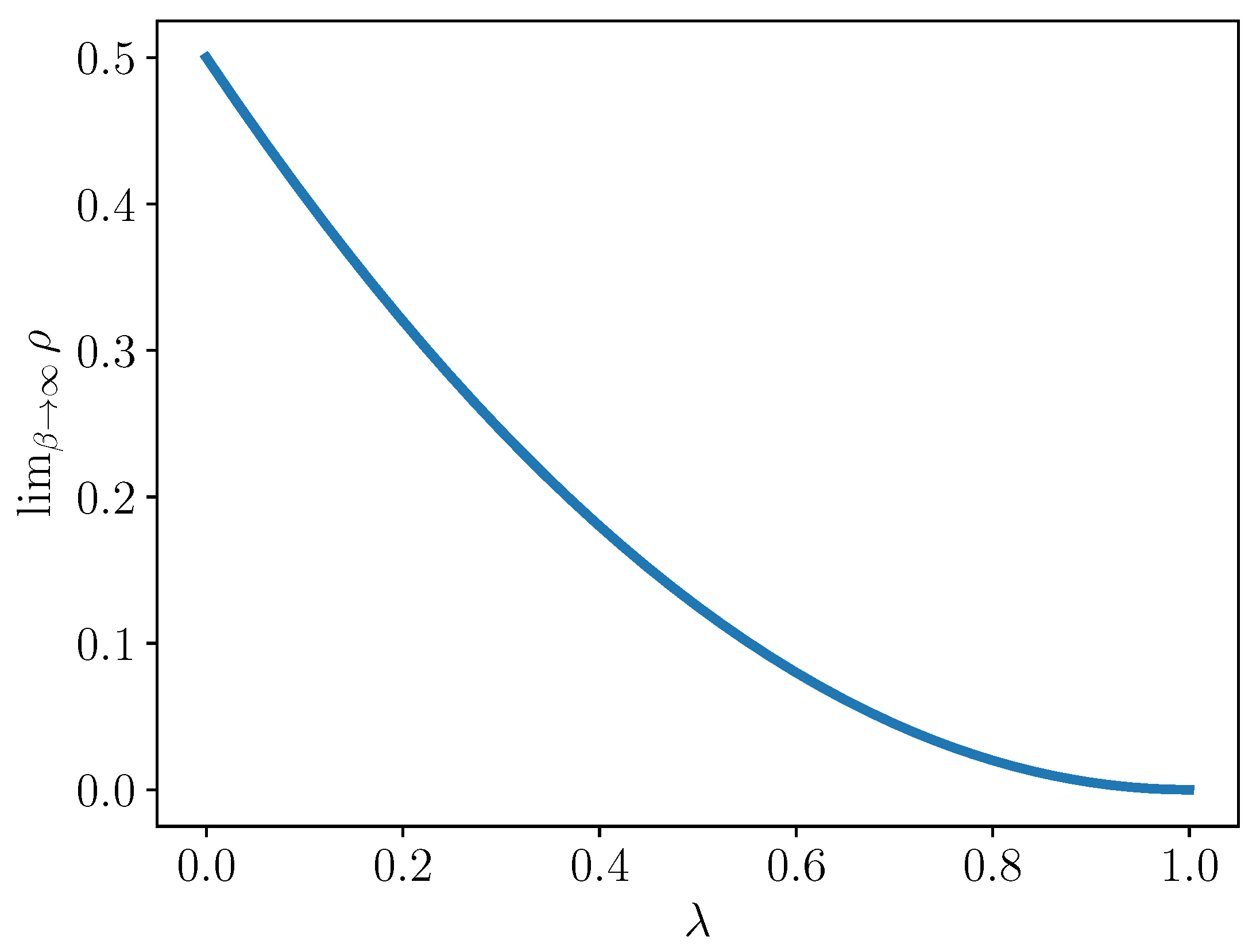
Let . Then,
Proof.
Given species in the original model, there are interaction terms, and . In terms of , , then is:
Then, the fraction may be written as:
In the limit as and for a fixed , we have:
□
This limiting value is plotted for in Figure 1. Note that in this limit, when , i.e., there is a complete reduction, then half of the interaction terms vanish. At the other extreme, when , i.e., so there is no reduction, then of course, all interaction terms can be nonzero.
Note that the conditions on the set and its complement are not necessary, but sufficient. They are not necessary at least in the sense of non-uniqueness: reordering the variables or making different substitutions could lead to a different set of zeroed interactions terms. However, the current results suggest at least some number of coefficients must be zero; otherwise, the entanglement of the species prevents exact reduction. We thus end this section with the following conjecture.
Conjecture 1
For -reducibility, it is necessary that at least terms are zero, where, for , .
4. Approximate Model Reduction
Motivated by the previous results, the final topic of this paper explored approximate model reduction. In this section, we consider the situation that information—interaction coefficients, growth rates, and some observations—is only available about a subset of out of species. We aimed to create an approximate model for those species without including any information about the excluded variables.
Interestingly, another recently developed method tackles the same situation: the focal species approximation (FSA) [9,29]. For an environment of S species, the FSA estimates interaction coefficients (from experiments) involving the species of interest and ignores the rest, thereby dropping the number of needed experiments from to . While the accuracy of this approximation is lower than that of the complete GLV model, the approximation still provides useful predictions and can thus be employed in applied settings for which full parameter estimation is infeasible. In a sense, the approximate AS and IS and the FSA demonstrate that (severely) reduced models may still capture the dynamics of interest within reasonable error.
4.1. Algebraic Substitutions
In the algebraic method, eliminated variables are exchanged for higher derivatives about the remaining variables.
Example 3
(Approximate AS for , ). The goal is to find an approximate model for , in terms of only .
The original model is, as before:
Motivated by the AS above, we write as an expansion in and its higher derivatives:
This leads to an approximate model for :
where and .
It may also be of interest to see the behavior of given the remaining terms from the original model, i.e., . We call this the naive reduced model. Note that this is the standard LV model if one only has access to the interaction coefficients of the reduced set of species.
Let us specify the coefficients of the original model as:
and set the initial conditions as and . (These values are approximate. The precise initial conditions were chosen randomly from a standard lognormal distribution.)
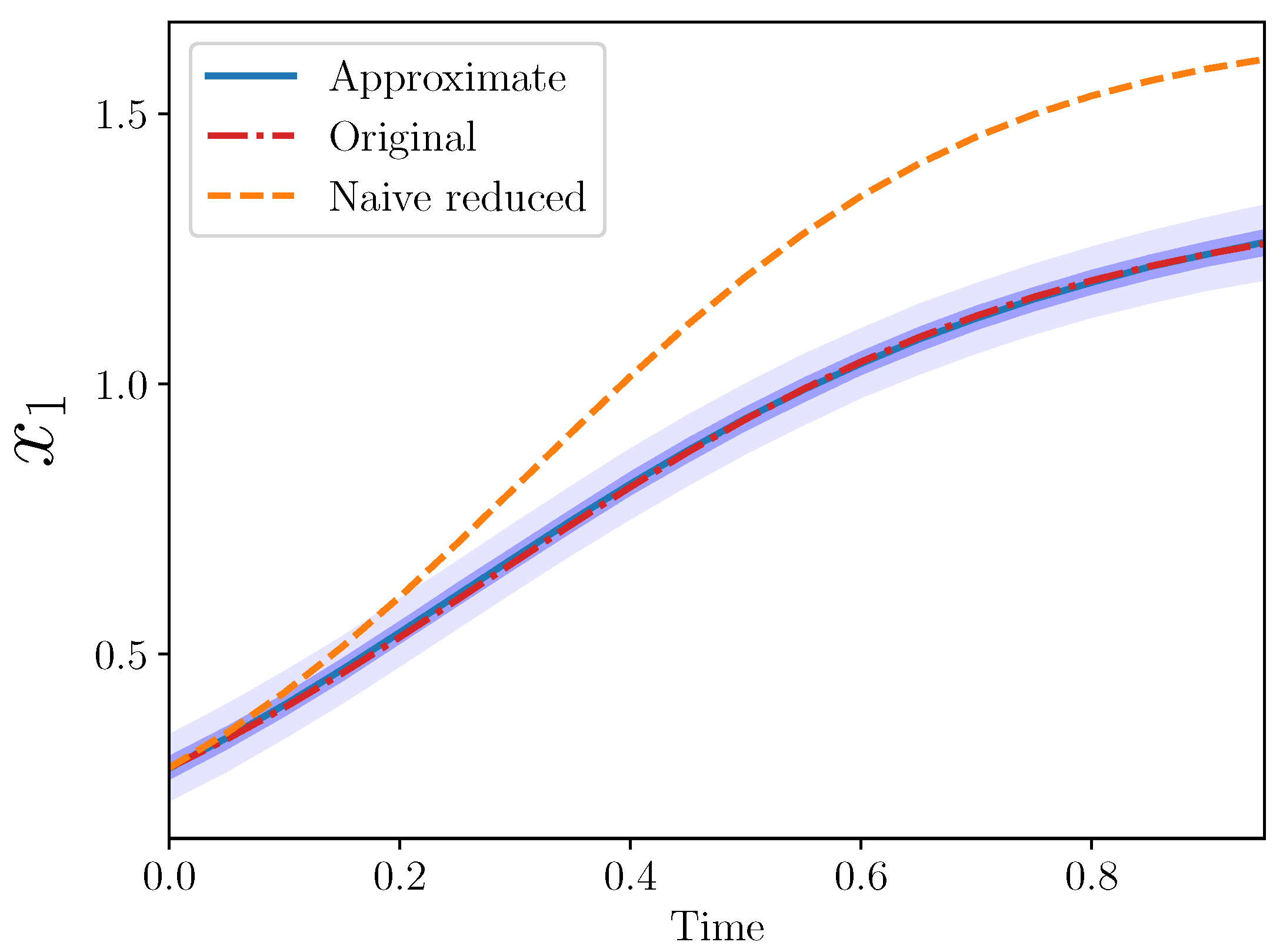
The introduced coefficients and are unknown and must be calibrated. We assumed data about over time. Calibration was performed under a Bayesian framework; the posterior means were and . The code to run Bayesian inverse and forward problems is available here: github.libqueso.com (accessed on 21 April 2021) [30]; specific implementations are provided in the supplementary material. The trajectory of is shown in Figure 2 from the three models: original, naive reduced, and approximate.
The approximate model is quite close to the original. Importantly, the approximate model output completely covers the original model output, which lies entirely within the approximate model 50% confidence interval.
Example 4
(Approximate AS for , .). Here, we tried the same framework with a slightly larger reduction: from three to one. In this case, note that we still replaced and with our approximate expression, but still only two new coefficients need be introduced.
Recall the original model for is:
The approximate model is then:
where and . Thus, we can again calibrate simply and .
Note the naive reduced model is again just:
Specifically, we set:
and the initial conditions to , , and .
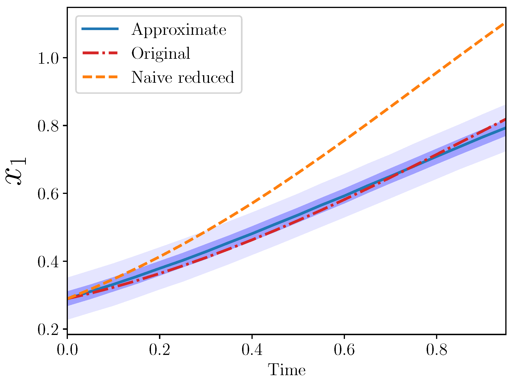
The posterior means were and . The trajectories from the three models are plotted in Figure 3.
Again, the approximate model is a good match to the original for . Note that ten coefficients from the original model were omitted (eight interaction and two growth rate coefficients), while only two new parameters were introduced, and .
4.2. Integral Substitutions
Another approach is instead inspired by the IS above, so that information about eliminated variables is replaced by memory, or integral, information of the remaining species.
Example 5
(Approximate IS for , ). Starting, as usual, with the original formulation:
we aimed for an approximate model by eliminating .
In this example, we also tried a slight variation from the algebraic one in that we replaced the entire term containing :
Moreover, since, in all of these examples, we assumed some data about the species of interest, we can approximate this integral directly from the data, which is generated according to the original model (and not the as given by the approximate model). In these numerical results, this integral was estimated numerically using a simple trapezoid rule. Call this numerical approximation :
where the ∗ in indicates that this integral was estimated from the data generated by the original model. Then, we pose the approximate model for as:
The posterior means in this case were and . The different trajectories for this example are shown in Figure 4.
Example 6
(Approximate IS for , ). Here, we present the final example, with the same original model as Example 4 (approximate AS for , ), and the same approximate model as the previous example.
Here we find and . The results are shown in Figure 5.
The approximate integral models also showed quite good agreement with the original model.
Note that each example here preserved the species correspondence: the species of interest was , and that is precisely what was modeled. This would readily generalize to approximate models for . While the resulting differential equations now include either a derivative or an approximate integral, the numerical solution is rather easily obtained without introducing much numerical complexity. In [31], Morrison provided an expanded investigation into similar AS-type approximate models.
5. Discussion
In summary, we can reduce a GLV system exactly by introducing integral terms of the remaining species or by introducing their higher derivatives. In a sense, some variables may be eliminated in exchange for this extra information about the reduced set. A few interesting results emerged from this work: First, a reduction from to variables is always possible. Second, a reduction from to is possible if the interaction terms in a specified set are zero. With , the fraction of terms in this set is approximately . Third, we saw that the two different methods in the case yielded a single ODE for , but either by maintaining the structure of the original ODE for or for . Fourth, after reducing to variables, an entanglement of species prevents further (exact) reduction without breaking the original model in some other way.
In this paper, this break was achieved by setting the interaction terms to zero. Of course, in some systems, this may be a reasonable assumption. This work also serves as a motivation for or evidence of how to approximate the role of the eliminated species using only the reduced set. The preliminary results suggested reduced models that they are no longer exact, but still preserve the species correspondence and are computationally feasible. A true validation test of this method would determine the accuracy and precision of the predictions with respect to real ecological (agricultural, chemical, etc.) data. Specific implementations and their effectiveness are an open and rich area for future study.
Supplementary Materials
To run forward and inverse problems for the approximate models, the code is available here: github.com/rebeccaem/enriched-glv [32].
Funding
This research received no external funding.
Data Availability Statement
Data is contained within the supplementary material.
Acknowledgments
I would like to acknowledge Tim Lyons, Sriram Sankaranarayanan, and Carl Simpson for many helpful discussions about this work.
Conflicts of Interest
The author declares no conflict of interest.
References
- Takeuchi, Y. Global Dynamical Properties of Lotka-Volterra Systems; World Scientific: Singapore, 1996. [Google Scholar]
- Wangersky, P.J. Lotka-Volterra Population Models. Annu. Rev. Ecol. Syst. 1978, 9, 189–218. [Google Scholar] [CrossRef]
- Dantas, E.; Tosin, M.; Cunha, A.C., Jr. Calibration of a SEIR–SEI epidemic model to describe the Zika virus outbreak in Brazil. Appl. Math. Comput. 2018, 338, 249–259. [Google Scholar] [CrossRef] [Green Version]
- Li, M.Y.; Muldowney, J.S. Global stability for the SEIR model in epidemiology. Math. Biosci. 1995, 125, 155–164. [Google Scholar] [CrossRef]
- Williams, F.A. Detailed and reduced chemistry for hydrogen autoignition. J. Loss Prev. Process Ind. 2008, 21, 131–135. [Google Scholar] [CrossRef]
- Jones, W.; Lindstedt, R. Global reaction schemes for hydrocarbon combustion. Combust. Flame 1988, 73, 3. [Google Scholar] [CrossRef]
- Frassoldati, A.; Cuoci, A.; Faravelli, T.; Ranzi, E.; Candusso, C.; Tolazzi, D. Simplified kinetic schemes for oxy-fuel combustion. In Proceedings of the 1st International Conference on Sustainable Fossil Fuels for Future Energy, Rome, Italy, 6–10 July 2009; pp. 6–10. [Google Scholar]
- Fort, H. Ecological Modelling and Ecophysics; IOP Publishing Limited: Bristol, UK, 2020. [Google Scholar]
- Fort, H. Making quantitative predictions on the yield of a species immersed in a multispecies community: The focal species method. Ecol. Model. 2020, 430, 109108. [Google Scholar] [CrossRef]
- Oberkampf, W.L.; Roy, C.J. Verification and Validation in Scientific Computing; Cambridge University Press: Cambridge, UK, 2010. [Google Scholar]
- Oliver, T.A.; Terejanu, G.; Simmons, C.S.; Moser, R.D. Validating predictions of unobserved quantities. Comput. Methods Appl. Mech. Eng. 2015, 283, 1310–1335. [Google Scholar] [CrossRef] [Green Version]
- Bayarri, M.J.; Berger, J.O.; Paulo, R.; Sacks, J.; Cafeo, J.A.; Cavendish, J.; Lin, C.H.; Tu, J. A framework for validation of computer models. Technometrics 2007, 49, 138–154. [Google Scholar] [CrossRef]
- Morrison, R.E.; Oliver, T.A.; Moser, R.D. Representing model inadequacy: A stochastic operator approach. SIAM/ASA J. Uncertain. Quantif. 2018, 6, 457–496. [Google Scholar] [CrossRef]
- Murdoch, A.I.; Bedeaux, D. Continuum equations of balance via weighted averages of microscopic quantities. Proc. R. Soc. Lond. Ser. A Math. Phys. Sci. 1994, 445, 157–179. [Google Scholar]
- Gear, C.W.; Kevrekidis, I.G. Projective methods for stiff differential equations: Problems with gaps in their eigenvalue spectrum. Siam J. Sci. Comput. 2003, 24, 1091–1106. [Google Scholar] [CrossRef] [Green Version]
- Mezić, I. Spectral properties of dynamical systems, model reduction and decompositions. Nonlinear Dyn. 2005, 41, 309–325. [Google Scholar] [CrossRef]
- Tartakovsky, A.M.; Panchenko, A.; Ferris, K.F. Dimension reduction method for ODE fluid models. J. Comput. Phys. 2011, 230, 8554–8572. [Google Scholar] [CrossRef] [Green Version]
- Haller, G.; Ponsioen, S. Exact model reduction by a slow–fast decomposition of nonlinear mechanical systems. Nonlinear Dyn. 2017, 90, 617–647. [Google Scholar] [CrossRef] [Green Version]
- Kazantzis, N.; Kravaris, C.; Syrou, L. A new model reduction method for nonlinear dynamical systems. Nonlinear Dyn. 2010, 59, 183. [Google Scholar] [CrossRef]
- Zhdanov, R. Higher conditional symmetry and reduction of initial value problems. Nonlinear Dyn. 2002, 28, 17–27. [Google Scholar] [CrossRef]
- Sahoo, S.; Garai, G.; Ray, S.S. Lie symmetry analysis for similarity reduction and exact solutions of modified KdV–Zakharov–Kuznetsov equation. Nonlinear Dyn. 2017, 87, 1995–2000. [Google Scholar] [CrossRef]
- Pavliotis, G.; Stuart, A. Multiscale Methods: Averaging and Homogenization; Springer: New York, NY, USA, 2008. [Google Scholar]
- Barabás, G.J.; Michalska-Smith, M.; Allesina, S. The effect of intra-and interspecific competition on coexistence in multispecies communities. Am. Nat. 2016, 188, E1–E12. [Google Scholar] [CrossRef] [Green Version]
- Grilli, J.; Adorisio, M.; Suweis, S.; Barabás, G.; Banavar, J.R.; Allesina, S.; Maritan, A. Feasibility and coexistence of large ecological communities. Nat. Commun. 2017, 8, 1–8. [Google Scholar] [CrossRef]
- Givon, D.; Kupferman, R.; Stuart, A. Extracting macroscopic dynamics: Model problems and algorithms. Nonlinearity 2004, 17, R55–R127. [Google Scholar] [CrossRef] [Green Version]
- Strogatz, S.H. Nonlinear Dynamics and Chaos with Student Solutions Manual: With Applications to Physics, Biology, Chemistry, and Engineering; CRC Press: Boca Raton, FL, USA, 2018. [Google Scholar]
- Harrington, H.A.; Van Gorder, R.A. Reduction of dimension for nonlinear dynamical systems. Nonlinear Dyn. 2017, 88, 715–734. [Google Scholar] [CrossRef] [PubMed] [Green Version]
- Hofbauer, J.; Sigmund, K. Evolutionary Games and Population Dynamics; Cambridge University Press: Cambridge, UK, 1998. [Google Scholar]
- Fort, H. Predicting The Yields of Species Occupying A Single Trophic Level With Incomplete Information: Two Approximations Based On The Lotka–Volterra Generalized Equations. bioRxiv 2021. [Google Scholar] [CrossRef]
- Prudencio, E.E.; Schulz, K.W. The parallel C++ statistical library ‘QUESO’: Quantification of Uncertainty for Estimation, Simulation and Optimization. In Proceedings of the Euro-Par 2011: Parallel Processing Workshops, Bordeaux, France, 29 August–2 September 2011; pp. 398–407. [Google Scholar]
- Morrison, R.E. Data-Driven Corrections of Partial Lotka–Volterra Models. Entropy 2020, 22, 1313. [Google Scholar] [CrossRef] [PubMed]
- Morrison, R.E. Rebeccaem/enriched-glv: Initial release. Zenodo 2020. [Google Scholar] [CrossRef]
Figure 1.
The fraction of the interaction that must be zero for exact reduction decreases nonlinearly as .
Figure 1.
The fraction of the interaction that must be zero for exact reduction decreases nonlinearly as .

Figure 2.
Approximate algebraic model for , . The darker blue band represents the 50% confidence interval (CI) and the lighter blue the 95% CI.
Figure 2.
Approximate algebraic model for , . The darker blue band represents the 50% confidence interval (CI) and the lighter blue the 95% CI.

Figure 3.
Approximate algebraic model for , .
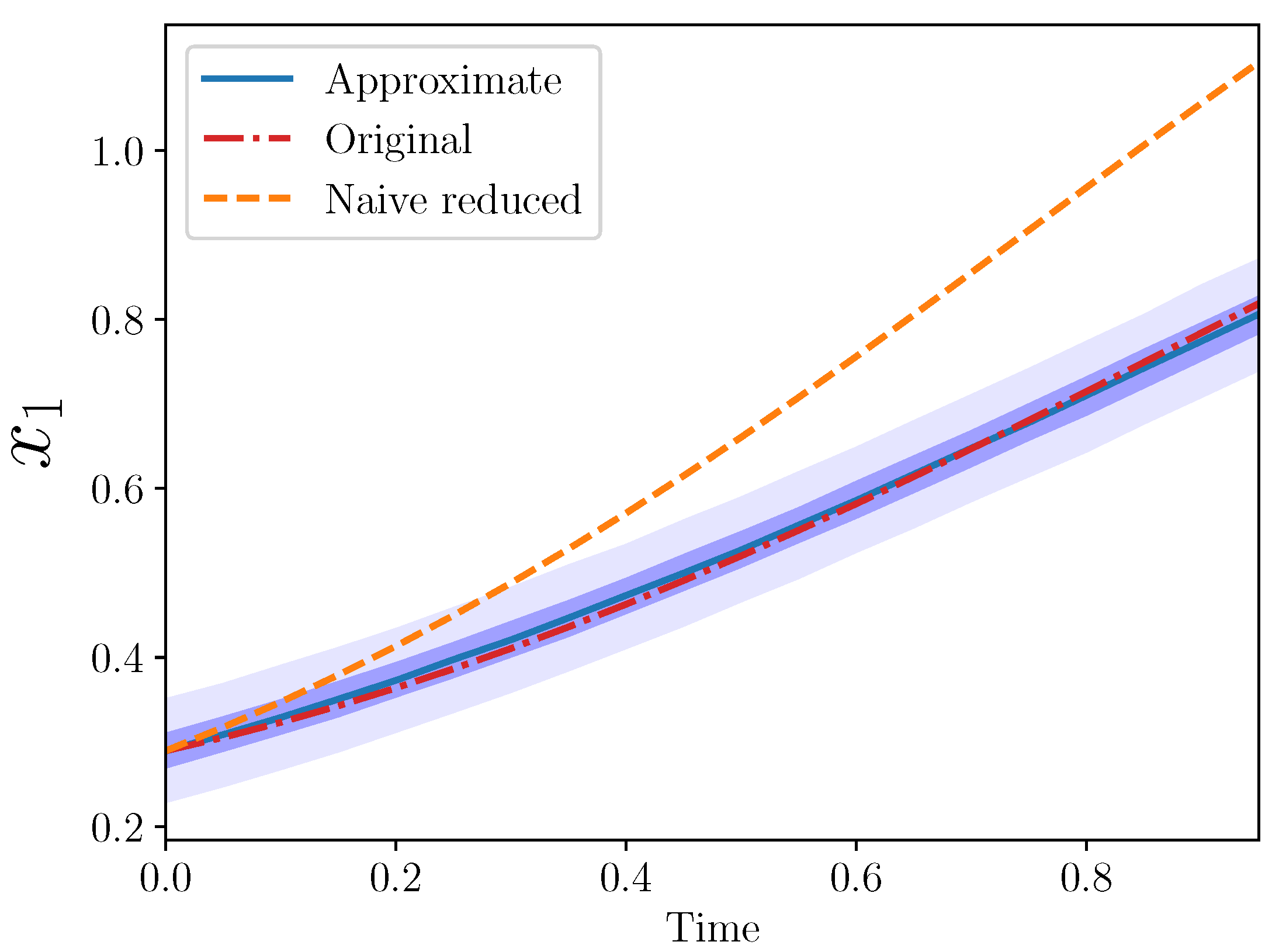
Figure 4.
Approximate integral model for , .
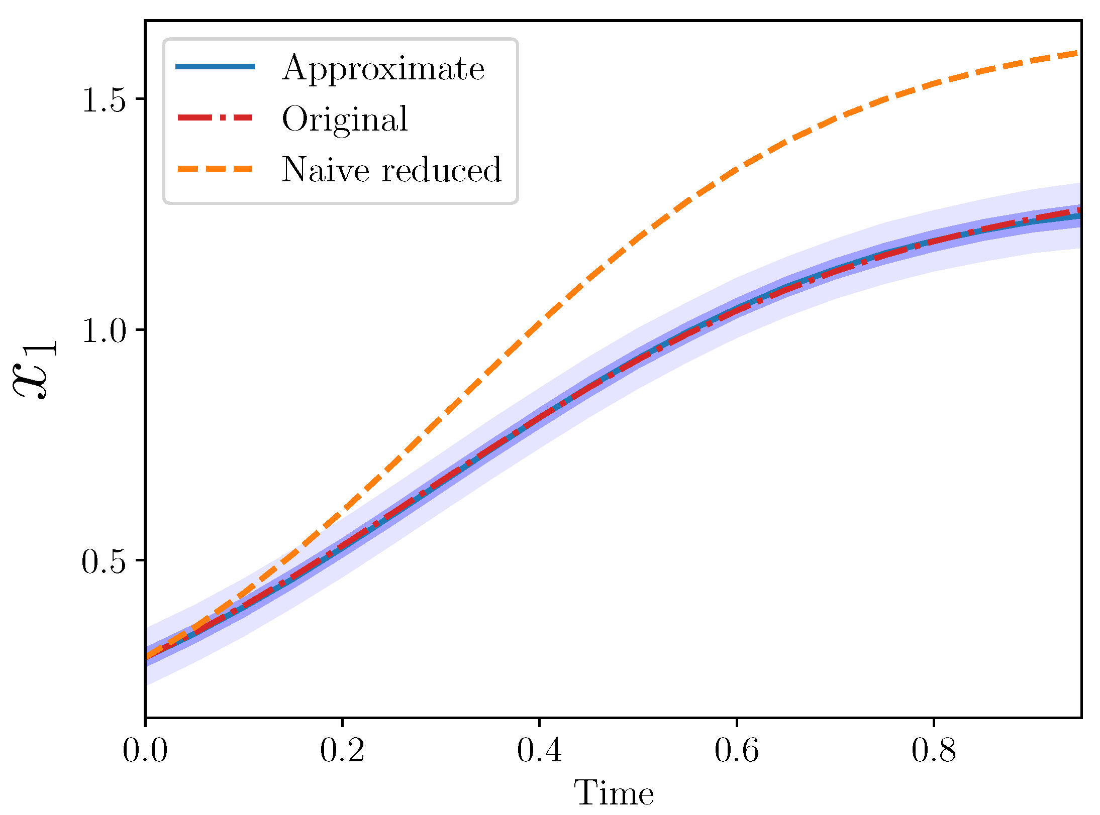
Figure 5.
Approximate integral model for , .

Publisher’s Note: MDPI stays neutral with regard to jurisdictional claims in published maps and institutional affiliations. |
© 2021 by the author. Licensee MDPI, Basel, Switzerland. This article is an open access article distributed under the terms and conditions of the Creative Commons Attribution (CC BY) license (https://creativecommons.org/licenses/by/4.0/).
Share and Cite
MDPI and ACS Style
Morrison, R.E. Exact Reduction of the Generalized Lotka–Volterra Equations via Integral and Algebraic Substitutions. Computation 2021, 9, 49. https://0-doi-org.brum.beds.ac.uk/10.3390/computation9050049
AMA Style
Morrison RE. Exact Reduction of the Generalized Lotka–Volterra Equations via Integral and Algebraic Substitutions. Computation. 2021; 9(5):49. https://0-doi-org.brum.beds.ac.uk/10.3390/computation9050049
Chicago/Turabian StyleMorrison, Rebecca E. 2021. "Exact Reduction of the Generalized Lotka–Volterra Equations via Integral and Algebraic Substitutions" Computation 9, no. 5: 49. https://0-doi-org.brum.beds.ac.uk/10.3390/computation9050049
Note that from the first issue of 2016, this journal uses article numbers instead of page numbers. See further details here.