
DrainCAN—A MATLAB Function for Generation of a HEC-RAS-Compatible Drainage Canal Network Model


Department of Hydroscience and Engineering, Faculty of Civil Engineering, University of Zagreb, HR-10000 Zagreb, Croatia
*
Author to whom correspondence should be addressed.
Computation 2021, 9(5), 51; https://0-doi-org.brum.beds.ac.uk/10.3390/computation9050051
Submission received: 26 February 2021
/
Revised: 1 April 2021
/
Accepted: 21 April 2021
/
Published: 23 April 2021
(This article belongs to the Section Computational Engineering)
Abstract
:The dimensioning of canal geometry in a surface drainage network influences the size and functionality of canal structures, reduces flood hazard, and consequently imposes restrictions on land use. Reliable free-surface flow calculation for optimization of the canal network can be challenging because numerous hydraulic structures and canal interactions influence the flow regime. The HEC-RAS software of the US Army Corps of Engineers’ Hydrologic Engineering Center is often used for this purpose as it allows the user to simulate the effect of numerous hydraulic structures on flow regime. This paper presents a MATLAB function, DrainCAN, for generating a HEC-RAS model from standard runoff input data, i.e., topographic data and canal design geometry (profile and slope). The DrainCAN function allows for fast optimization of the network geometry—it generates normal flow depth estimation and observed water levels in critical locations that need to be optimized. Advantages of the DrainCAN function are fast generation of the HEC-RAS hydraulic model files from simple input files, introduction of optimization variables in the model, and automatic adjustment of model geometry for computational junctions. This allows fast iteration of the canal design parameters, namely cross-sectional geometry, invert elevation, and longitudinal slope, and the evaluation of introduced changes on the flow regime.
1. Introduction
Efficient water resources planning and management is crucial for establishing a sustainable water distribution scheme between competing users, among which agriculture is the largest consumer of the water resources, whereby 70% of global water withdrawals are for irrigation purposes [1]. It is estimated that more than 60% of all water withdrawals for irrigation returns into local aquifers, either through drainage of excess water or groundwater percolation [2]. Although the primary purpose of the drainage canal network is to control flooding, water ponding, and waterlogging in order to preserve the agricultural land, the multiple uses of water from the drainage canal network (i.e., for irrigation in many water scarce areas [3]) imply that all uses must be considered in the design process to solve water distribution and quality problems. Therefore, hydraulic calculation of water surfaces in the canal network is crucial in the design process to ensure the required canal capacity while, at the same time, minimally restricting land use.
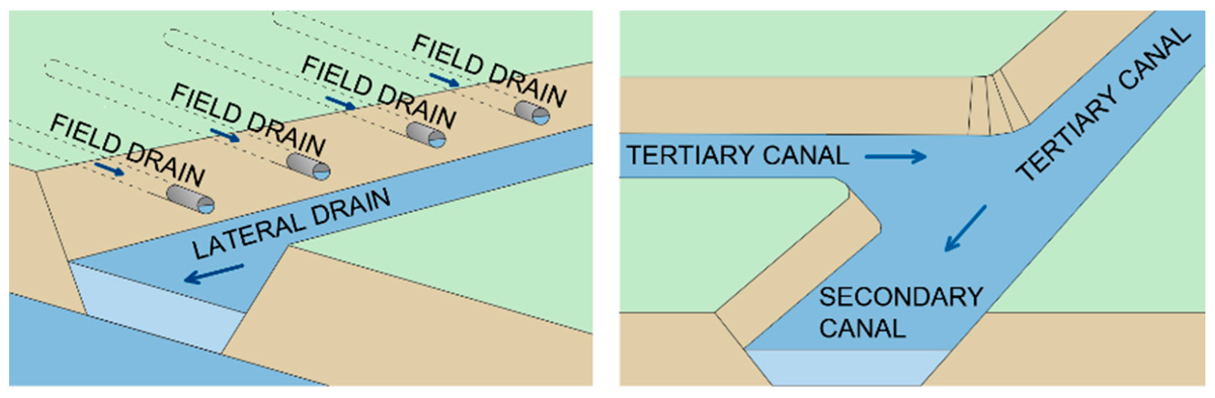
Generally, a drainage system can be divided into the field drainage system, main drainage system, and outlet [4]. The purpose of the field drainage system is to control waterlogging and/or water ponding by collecting excess surface and subsurface runoff in the lateral and field drains, respectively. The main drainage system is a network of open canals: tertiary drain that collects water from the field drainage system while primary and secondary drains transport the water to the outlet point. The outlet of the main (primary) drain is the exit point of the system, where excess water is discharged into the recipient (Figure 1).
Drainage canal network complexity is characterized by the multiple lateral confluences of lower order canals into the higher order canals (Figure 2). The drainage canal network is usually designed according to the following hierarchy: lateral drains collect inflow from series of field drains, whereas primary, secondary, and tertiary canals collect the inflow from all canals of lower order than their own. When two canals of the same order intersect at a junction, they form a canal of higher order that continues downstream. Drop structures are usually placed at this junction to compensate for an increase in geometry of the higher order canal. Two lateral canals cannot intersect—they must always produce an inflow into the one of the higher order canals.
Lateral drains are, from the hydraulic perspective, generally overcapacitated—they need to be deep enough to allow inflow of field drains without receiving backwater flow while allowing clearance for siltation of washed away soil particles [5]. Their geometry, in turn, influences the invert of the higher order canals that needs to be deepened to allow inflow. To maintain optimal water regime in canals, flow-regulating structures are constructed, such as weirs, gates, and drops, at the outlet of lower order canals into higher order canals. This distinguishes them from rivers and theoretical flow in canals, highlighting the need for use of numerical models in the design process to shorten the time for iterative geometry design to a minimum. One of the most frequently used software packages for free-surface flow simulation is the Hydrologic Engineering Center’s River Analysis System (HEC-RAS), developed by the US Army Corp of Engineers in 1995 [6]. HEC-RAS is a software application for 1D, 2D, or combined 1D/2D hydraulic simulations in steady and unsteady flow regime, 1D sediment transport, and morphodynamic channel development, water quality analysis, and hydraulic design. Advantages of HEC-RAS are versatility (simulation of the flow through a network of open channels with pertaining hydraulic structures—bridges, weirs, gates, storage areas, levees, diversions, etc.), user-friendly GUI, and continuous upgrades while use of the software is free of charge.
Agudelo Otálora et al. [7] determined that both 1D HEC-RAS and an artificial intelligence model based on artificial neural networks (developed in MATLAB) accurately estimate flood flows. Although the advantages of HEC-RAS make it most suitable for use in a riverine environment, e.g., estimation of flood levels along the river reach [8], its applicability to small-scale open channels has also been demonstrated: Marimin et al. [9] applied HEC-RAS to study small-scale flooding in the Sembrong river catchment area, while Buta et al. used HEC-RAS and HEC-GeoRAS to simulate flash flooding in a small drainage basin [10]. The versatility of HEC-RAS can be seen in various research applications. It was successfully used for flash flood simulation where subcritical flow can occur (e.g., [11,12]). HEC-RAS is extensively used in agriculture for drainage and irrigation optimization. Baky et al. [13] successfully used HEC-RAS to produce flood hazard maps for an agricultural area. Raslan et al. [14] used a HEC-RAS 1D model to compare the effectiveness of each of the three alternative hydraulic solutions of a water reuse approach in a reclamation project in northwest Sinai. They successfully implemented HEC-RAS for modeling flow in canal controlled by different types of structures and drops. Traore et al. [15] used HEC-RAS and to set up a hydraulic model of four streams connecting the reservoirs used for irrigation. As already mentioned for drainage networks, siltation can play a significant role on canal conveyance as well as vegetation growth. Kiesel et al. [16] applied the three-step cascade model to simulate impacts of environmental changes on water and sediment fluxes for the agriculturally used lowland catchment in Germany. A HEC-RAS 1D hydraulic model was used to simulate channel erosion and sedimentation from the catchment to the micro-reach scale, and they found that HEC-RAS results agree well with the observed data both for streamflow and sediment transport. Sennaoui et al. [17] used 1D HEC-RAS to estimate sedimentation in the agricultural drainage canal of a wetland northeast of Algeria. Their reported findings showed that the sedimentation occurred not only during floods but also continually after rainfall events, thus reducing the canal capacity. King County Department of Natural Resources and Parks [18] investigated the effects of dredging in the drainage canals on the adjacent agricultural lands. They found that the HEC-RAS model had much higher roughness coefficients than typical (due to the growth of excess vegetation) and proposed the methodology to predict the post-dredge water levels. Nemati Kutenaee et al. [19] used HEC-RAS to calculate the effect of the Caspian Sea water level variations on drains with sea outlets. Xiao et al. [20] compared the performance of HEC-RAS and QUAL2K (River and Stream Water Quality) models for estimation of nutrient discharges in a constructed wetland. They found that HEC-RAS simulation produced results that had smaller differences from onsite field data when compared to QUAL2K.
Despite advancement in numerical modeling of free-surface flow, various 1D hydrodynamic models are still go-to solutions when flow simulation is required for water level calculation in prismatic channels, flood level forecasting or water regime analysis on long river reaches. Advantages of a 1D model over 2D or 3D models are in more straight-forward geometry definition, simple boundary condition assignment, and fewer coefficients used for numerical solution, while the flow characteristics—average flow depth and velocity—obtained from the 1D and 2D analysis for simple channels are reported to be similar [21,22]. Some users manage to extend HEC-RAS beyond its capabilities through coupling with compatible software, e.g., coupling with ArcView for flood risk analysis [23], with flood wave dynamic models for dam break analysis [24] or with MODFLOW to simulate groundwater and surface water interaction in the shallow aquifer [25]. Advanced users can make use of third-party software to externally control and/or automate HEC-RAS simulations. The control of HEC-RAS simulations is possible using the HEC-RAS Controller (collection of classes, functions, and subroutines) [26]. Dysarz [27] presented advantages of using a Python script to control HEC-RAS due to access to geoprocessing tools essential for flood hazard mapping. Saeed [28] coupled LARSIM and HEC-RAS into a hydrological–hydraulic model for usage in flood forecasting for upper main catchment. Saeed automated a HEC-RAS model in the flood forecasting tool using MATLAB, where input data were imported from the existing MIKE11 model. The tool has the capability to extract the observed and LARSIM simulated data, to write the HEC-RAS input files, to run and calibrate the model with randomly generated Manning’s values and, finally, to plot the water levels at the user-specified bridges. In his PhD thesis, Albo-Salih [29] developed a methodology for operation management for releases through control gates of river–reservoir systems during floods in real-time. The methodology coupled together a genetic algorithm coded in MATLAB with 1D and 2D HEC-RAS simulations. Reinoso-Gordo et al. [30] developed an open-source algorithm for calculating flow accumulation based on a CPU approach. The advantage of their approach is the use of a free software alternative to MATLAB, Octave.
The model geometry for HEC-RAS can be defined in several different ways, from the basic manual input of X and Y cross-sectional data pairs to integration with Arc-GIS to derive steam cross-sections from a digital elevation model (DEM) [31]. Gichamo et al. [32] highlighted the need for high-quality data or extensive pre-processing when GIS is used for terrain formation. HEC-GeoRAS can be used to process geospatial data in ArcGIS to create HEC-compatible geometry, but an ArcGIS license and extensive input data are required to create a DEM. During the design of a drainage canal network, the canal corridor is overlapped (superimposed) onto the DEM at locations of control cross-sections to derive the canal geometry used in the optimization process. The size of the DEM affects the computation requirements, limiting the application when fast analysis is necessary [30]. Users often resort to HEC-RAS for small-scale projects that have a limited budget and, therefore, the creation of complex DEMs or coupling with licensed software is not feasible. Therefore, in order to complement HEC-RAS’s free availability, users often have a need for a simple, reliable tool for fast analysis in smaller-scale applications.
This paper presents the MATLAB function DrainCAN for creating model geometry and flow data for input in HEC-RAS and subsequent use in drainage canal network optimization. During the canal design process, the designer needs to evaluate the hydraulic efficiency of different canal geometries (altering both cross-sectional profile and longitudinal slope) as well choose the appropriate roughness for the model (based on the selection of canal lining-cleared, grassed, concrete, geomembranes, etc.). DrainCAN tool enables the creation of HEC-RAS geometry, fusing only basic input from the designer–cross-sectional geometry of the canal outlet and longitudinal slope (for each canal), topographic layout of the canals with desired locations of cross-sections, and selected Manning’s roughness coefficient. Manning’s coefficient can be altered in the later stages within the HEC-RAS environment for each of the hydraulic runs according to requirements. HEC-RAS has the option to set Manning’s coefficient individually between any two geometry points of the cross-section, which gives the designer the option to set different roughness for the canal bottom and each bank slope and evaluate the influence of different linings on the water levels.
The aim of the research was to develop a free function for use in the optimization process of the canal geometry, exploiting the full functionality of the HEC-RAS software. The focus of the DrainCAN function is on the generation of HEC-RAS input files, with simultaneous incorporation of optimization variables such as observed water surface elevations, normal depth calculation, and extraction of terrain topography at canal cross-sections.
2. Methodology
HEC-RAS uses a number of input parameters for hydraulic simulation that are required to be defined in two files and associated with the run plan: the geometry file and the flow file. In the geometry file, a series of cross-sections along the stream axis is defined in absolute coordinates to comply with external data, such as gauging station recordings or land use data. The minimum requirement for each cross-section is to define two points that are dedicated banks, the downstream distance to next cross-section and the roughness coefficient. In the flow data file, the minimum requirements are two boundary conditions—on the most upstream and most downstream cross-section. Additionally, the flow change can be introduced at any given cross-section as well as observed water levels for model calibration/optimization. The structure of the DrainCAN function is outlined with a detailed description of the MATLAB script functionality broken down into independent blocks as follows. Firstly, input data are introduced into the MATLAB environment. Secondly, the geometry for each canal is constructed. Thirdly, intersections of canals are determined to create junctions. Finally, the output from the function is externally saved HEC-RAS input files. Each block includes a set of error-check procedures in order to achieve function robustness.
Input data that need to be prepared before running the function consists of land topography (DTM), drainage canal network scheme (CNS), and canal geometry with inflow data (CGI) from rainfall–runoff calculation. The user is prompted to select the input data one at a time from local storage. Land topography is vectorized as 3D points, lines, or polylines (both 2D and 3D) created with software capable of exporting entities in drawing interchange format (.dxf). Land topography must cover the corridor of the drainage canal network in order to represent the terrain elevations at the location of computational cross-sections. If the canal network layout is also susceptible to change in the optimization process, land topography should be defined in such a way that spans across the domain under which the canal network layout is acceptable.
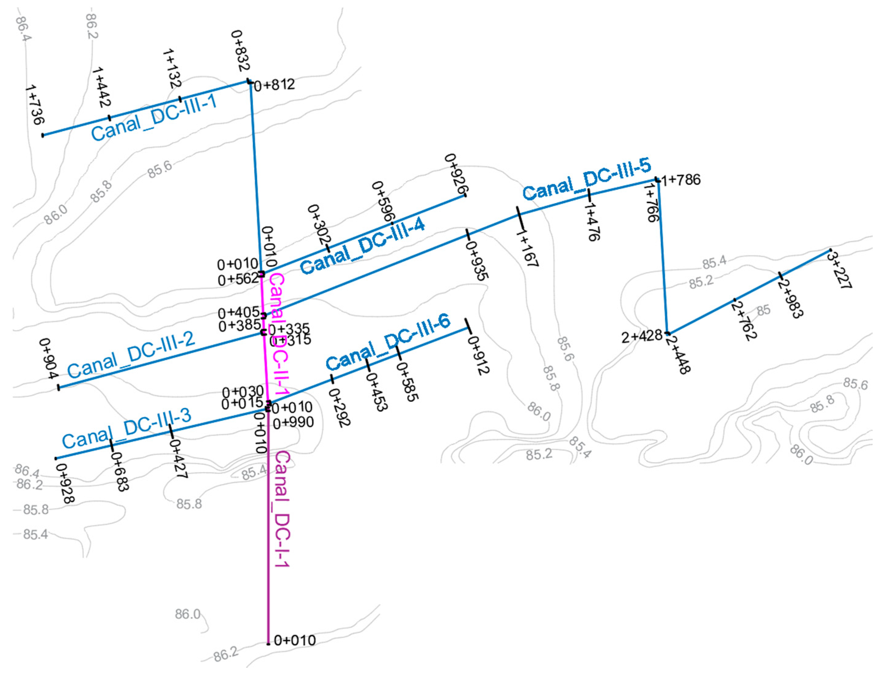
Drainage canal network scheme outlines the primary, secondary, and tertiary drain network, while lower order lateral drains are not part of the computation scheme. The scheme of the drainage network is shown in Figure 3. Drainage canals are drawn in a CNS file as a continuous polyline starting from the drain’s respective starting point (most upstream) to the drain end (outlet). The naming convention for canals in the network is that unique canal IDs are constructed with a series of strings consisting of “DC” (acronym for drainage canal), drain order in Roman numerals (“I”, “II” or “III” for primary, secondary, and tertiary drain, respectively) and canal ordinal number in a continuous sequence (“1”, “2”, “3”, etc.), connected with dashes to form a unique name for each canal in the hierarchy, e.g., “DC-I-1”. The script performs control of the input data in the CNS file if at least one primary canal exists, and are all canals are drawn as polylines.
Lateral drains collect inflow from the field drains which, from the hydraulic perspective, accumulates to relevant flow at the outlet of the lateral drain. Therefore, the hydraulic calculation for flow in the lateral drain is redundant—for the purpose of the agricultural drainage lateral drains are all considered to be uniform. Moreover, estimation of the siltation in lateral drains surpasses the detail needed for hydraulic simulations and, therefore, is estimated for each canal. Taking all these restrictions into account, lateral drains are represented by two variables—canal depth and flow depth. These variables are used to calculate absolute canal elevation at the confluence, which is defined as cross-section in the CNS file. Computationally, each defined cross-section presents inflow from the lateral drain and will be assigned as flow change location in the HEC-RAS together with the observed water level.
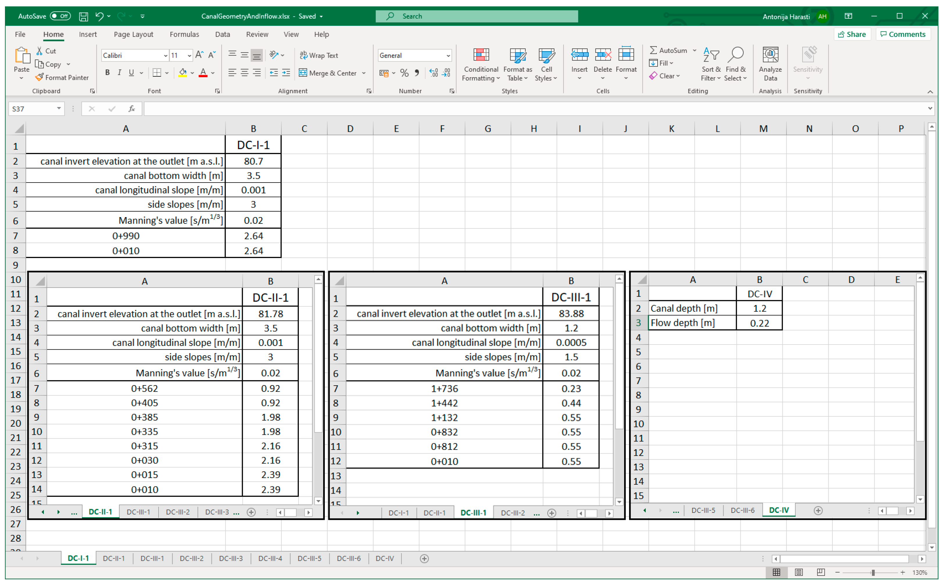
The input CGI file (.xls) has the structure describing the main geometric characteristics of each canal (bank slopes, bottom width, canal longitudinal slope), estimated roughness coefficient, and inflow from lateral drains for each cross-section (Figure 4). The Excel file was selected as input because it was shown to be the most intuitive input during the testing phase. Since the main purpose of the DrainCAN function is to produce HEC-RAS geometry in the optimization process, it means that the designer will create several geometries and perform hydraulic calculations until the optimal geometry is reached while retaining design runoff data for the most part. When the drainage network consisted of large number of canals, Excel worksheets were preferred as input as they are compatible with rainfall–runoff calculations.
Script searches for higher order drains in the CGI file were used to check the compatibility with the CNS file—if all existing canals match by name, and if all stations are drawn in a canal network. For each secondary and tertiary canal in the network, the normal depth on its outlet is calculated. This value will be drawn in the HEC-RAS model as “observed water surface elevation” in order to evaluate if there is backwater flow in the canal in the optimization process.
Each cross-section is assigned with the corresponding flow data from the CGI file. Each canal in the network has a separate worksheet of the CGI input file, where the design data are defined to be used for HEC-RAS model creation. The worksheet name reflects the name of the canal it is associated with (Figure 4). For each canal, the designer writes in the desired geometric parameters (from top to bottom): canal invert at the outlet [m a.s.l.]; bottom width [m]; longitudinal slope [m/m]; side slopes (V:H) [m/m]; Manning’s roughness coefficient [s/m1/3], and inflow from lateral canals on each cross-section [m3/s].
The flow in the lateral drains consists of surface runoff directly into lateral drains and subsurface runoff as point inflow from field drains. This phenomenon exceeds HEC-RAS functionality and must therefore be calculated outside its environment and used as flow file input. Surface runoff can be simulated using the Hydrologic Modeling System (HEC-HMS), which has output compatible with HEC-RAS flow file input. HEC-HMS requires basin model files, meteorological model files, and soil and land use/cover that can be created by the HEC-GeoHMS plugin [33]. Surface runoff can be simplified using empirical formulae that have fewer input parameters representing catchment characteristics, but it will affect the accuracy. The same is true for subsurface runoff (inflow from tile drains), but its contribution is significantly smaller and has a time lag which makes it less relevant for calculation of peak runoff volumes. In our research, we used data from a master’s thesis [34] as inflow data.
The first block of the DrainCAN function checks if all canals have associated cross-sections—the minimum required number of cross-sections in order to perform hydraulic simulation is 2. Canal invert elevation at each cross-section is calculated using the canal invert at the outlet and slope provided in the CGI file with corresponding distance from the outlet. The cross-sectional geometry is then constructed using the canal bottom width and bank slopes. The cross-sectional geometry is saved in absolute coordinates as 3D points (X, Y, Z). This allows overlapping with terrain points from DTM and extracting the corresponding terrain elevation at the location of the respective cross-section. The end of the cross-section geometry is defined by the bank station at the intersection of the bank slopes with the DTM. If the script determines that the canal invert is higher than the terrain at the cross-section location (resulting from assigned steep canal slope), the script returns a message box with error metadata (error type, canal ID, cross-section ID) and the function terminates. The final characteristic of the cross-section is distance to the adjacent downstream cross-section, which is calculated from the axial distance between two adjacent cross-sections.
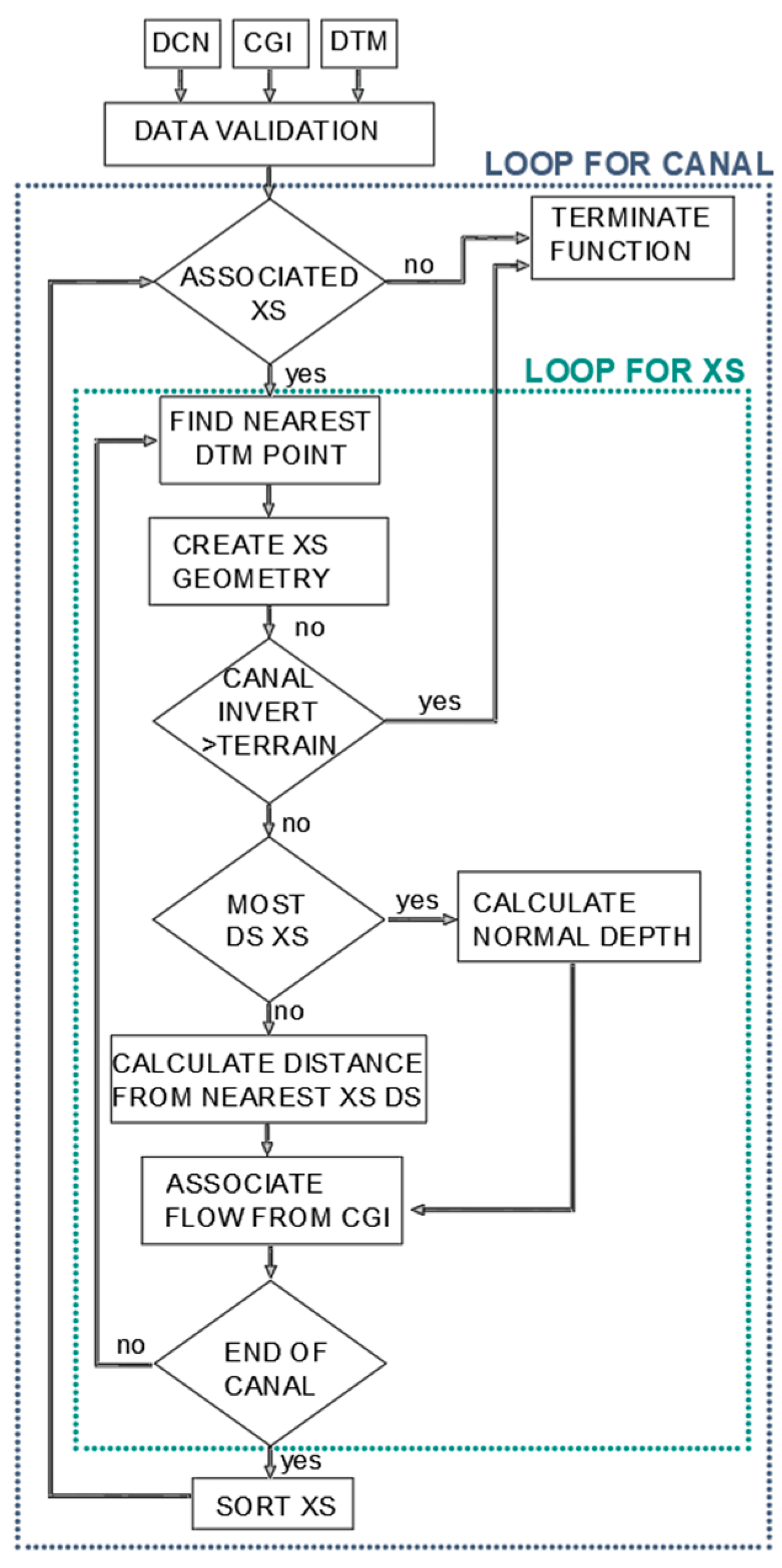
Within the DrainCAN function, several nested functions are used for importing external data or solving geometrical problems, such as finding the intersection of lines in 3D space, projection of points onto lines, etc. For these purposes, the existing functions published on user-developed code exchange platforms were used and modified to comply with DrainCAN requirements: for importing canal network and terrain generated as .dxf file [35], projection of a point onto a line [36] after calculating the distance between them [37], and calculating normal depth for standard canal cross-sections (trapezoidal, rectangular and triangular) [38]. The flow chart of the first block function is given in Figure 5.
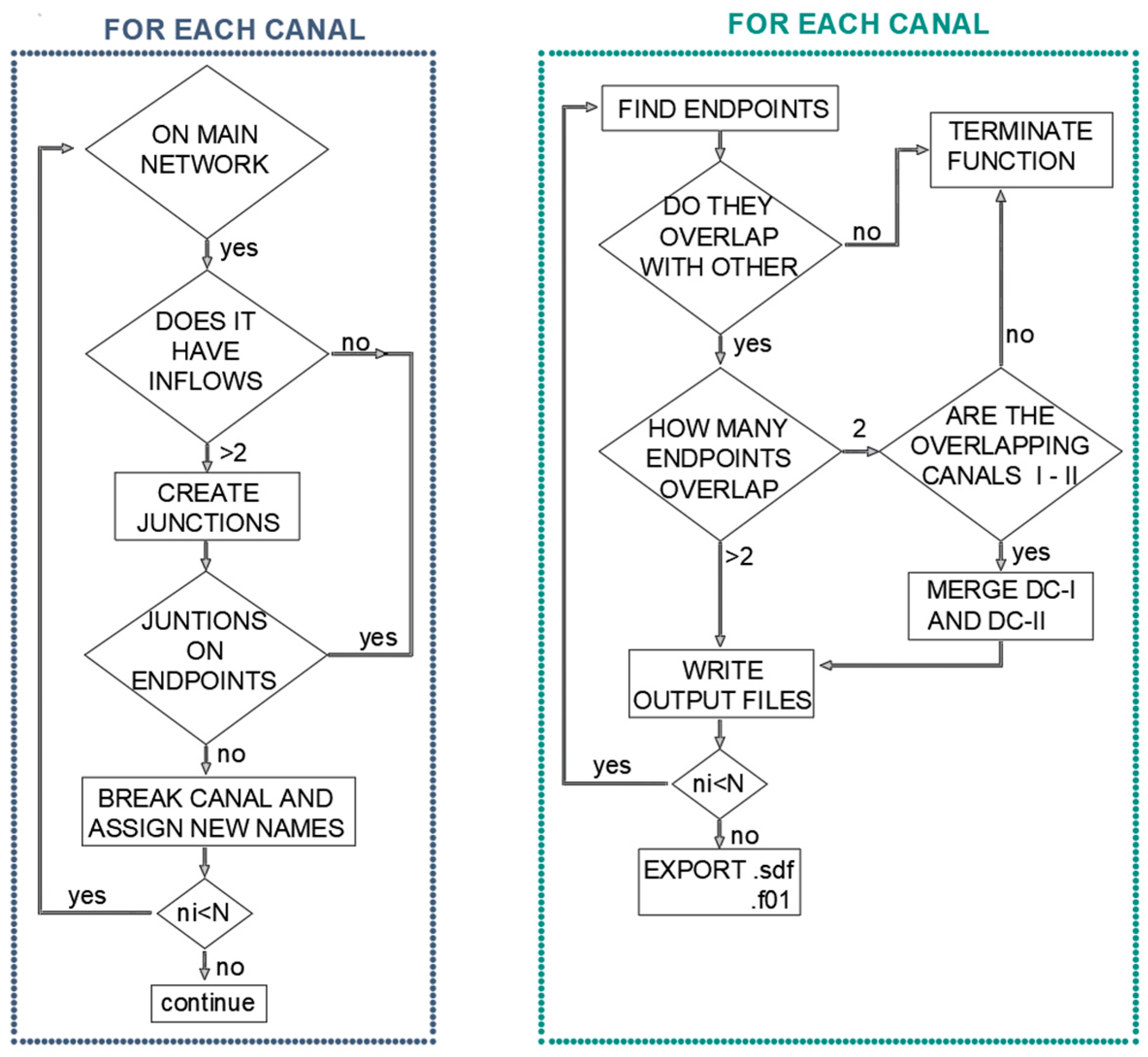
The drainage canal network differs from the river network in multiple canal interaction, while river confluences are less common and spatially positioned further apart. HEC-RAS treats each confluence as a computational junction that needs to be defined with a unique canal ID for entering and exiting the junction. Therefore, when a higher order canal has lateral inflows from multiple lower order canals, each inflow must be defined as a junction. The canal between the junctions has to be assigned with a unique name, even if it is nominally the same canal. The following block (Figure 6) of the function is used to find lateral inflows into higher order canals and to divide the canal into series of canals between the junctions while preserving the given name with assigning the ordinal number for each of them. E.g., canal “DC-II-1” will become series of canals named “DC-II-1(1)”, “DC-II-1(2)”, etc. In order to account for human error in drawing intersections, the tolerance for canal intersection is set to 5 m.
The following function block writes the .sdf file that can be directly imported in HEC-RAS as a geometry for calculation. The flow chart of the function block that writes output files is given on Figure 6. Structure of HEC-RAS import file was modeled after the HEC-RAS User’s Manual [39]. Appendix B of the HEC-RAS User’s Manual describes HEC-RAS import/export files for geospatial data (RASImport.sdf) which is a structured text file composed of several sections. Goodell has also highlighted advantages of manipulation of the HEC-RAS data files in ASCII format [40]. For the .sdf import file, the end points of each canal reach are firstly defined as start and end points. Locations where 3 or more start/end points overlap are identified as junctions and given a unique junction ID. At this point, one more control point is introduced—users frequently continue with the primary canal directly after the secondary as the primary canal is often part of some existing network and may be of different geometry. If that is the case, the user has selected creating a junction with only two reaches, which is not supported by HEC-RAS. Since this junction does not present an error from the engineering perspective, the function is not terminated and, rather, the geometry of the secondary canal merged with the primary canal to be preserved “as is” under the primary canal designations. After that, all the data collected about the reach axis and corresponding cross-section is written according to the .sdf file structure requirements. First, the stream network is created, then cross-sections. Finally, the steady flow file is created to correspond with the created geometry. The function will assign normal slope as a downstream boundary condition, while streamflow is upstream flow condition, as well as inflow on each cross-section being defined in the CGI file.
MATLAB was selected for development of the DrainCAN function because it is commonly used in the engineering community—one of the greatest advantages of MATLAB is its open code that can be shared between users in the MATLAB Central community without any cost. This community ensures that functions can be frequently updated through two-way interaction between the developers and users—the feedback code can be improved on this basis, and subsequent updated versions published. The DrainCAN function runs on the basic version of MATLAB (no additional toolboxes required) and is therefore compatible for running in the Octave environment as well.
3. Results and Discussion—Case Study
In this section, a working example of the function is presented that was tested in two master’s theses, namely on a case study [34] and in general testing of the function [41]. The case study selected for the illustration of DrainCAN functionality is agricultural area located in Velika Kopanica (Croatia) covering 685 ha of land. This lowland area is adjacent to the main recipient, Sava River, with terrain elevation between 85 and 87 m a.s.l. The layout and geometry of the drainage canal network reflects the existing constructed state: the main drainage network consists of six tertiary canals (DC-III-1 to DC-III–6), one secondary (DC-II-1), and one primary canal (DC-I-1) with outflow into the recipient. The secondary canal begins at the junction of the two tertiary canals (DC-III-1 and DC-III-4) located furthest from the recipient. The secondary canal continues downstream while other tertiary canals inflow laterally into it, with the last one (DC-III-3) inflowing at the end of the secondary canal. From this point onwards, the primary canal transports the runoff directly into the recipient. A scheme of the existing drainage network is shown in Figure 7.
All canals have trapezoidal cross-sections—tertiary canals have a bottom width of 1.2 m and a side slope of 1.5, while primary and secondary canals have the same geometry with a bottom width of 3.5 m and side slope of 3. Cross-sections of the tertiary canals represent inflow from the lateral canals which are uniformly distributed and averagely spaced every 300 m. Tertiary canals 1–5 collect inflow from 6, 1, 3, 3, and 12 lateral drains, respectively. All 30 lateral drains are 1.2 m deep, and the estimated depth water in them is 0.22 m. The geometry created by DrainCAN function is imported into HEC-RAS under “Geometric data” editor, using “File→Import Geometry Data→GIS Format” and then selecting the HEC-geometry.sdf file.
Flow data selected for simulation is the maximum runoff calculated from design rainfall. Runoff was calculated using empirical equations, accounting for surface and subsurface runoff for each lateral drain while flow in the primary network was adjusted for hydrograph lag. Inflow data for this case study was retrieved from master’s thesis [34] and structured for input as shown on Figure 8.
In Methodology (Section 2), it was explained how DrainCAN (Figure 6) creates junctions on secondary canals at locations where one or more tertiary canals inflow into them. In this case study, the secondary canal DC-II-1 has lateral inflows from tertiary canals and, thus, the secondary canal must be divided into separate sections while maintaining its original designation. Since the DC-II-1 is intersected by three tertiary canals (DC-III-5, DC-III-2, and DC-III-6), it is divided into four new sections: DC-II-1(1) between inflows of DC-III-3 (end of the canal) and -6, DC-II-1(2) between inflows of DC-III-6 and -2, DC-II-1(3) between inflows of DC-III-2 and -5, and DC-II-1(4) between inflows of DC-III-5 and the start of the canal. Even though the sections of the secondary canal have different names, they still represent the original geometry of DC-II-1 and its flow continuity is retained. Flow input data created by the DrainCAN function is imported into HEC-RAS under “Main window”, using “File→Import Data→HEC-RAS Data” and then selecting the HEC-flow.f01 file.
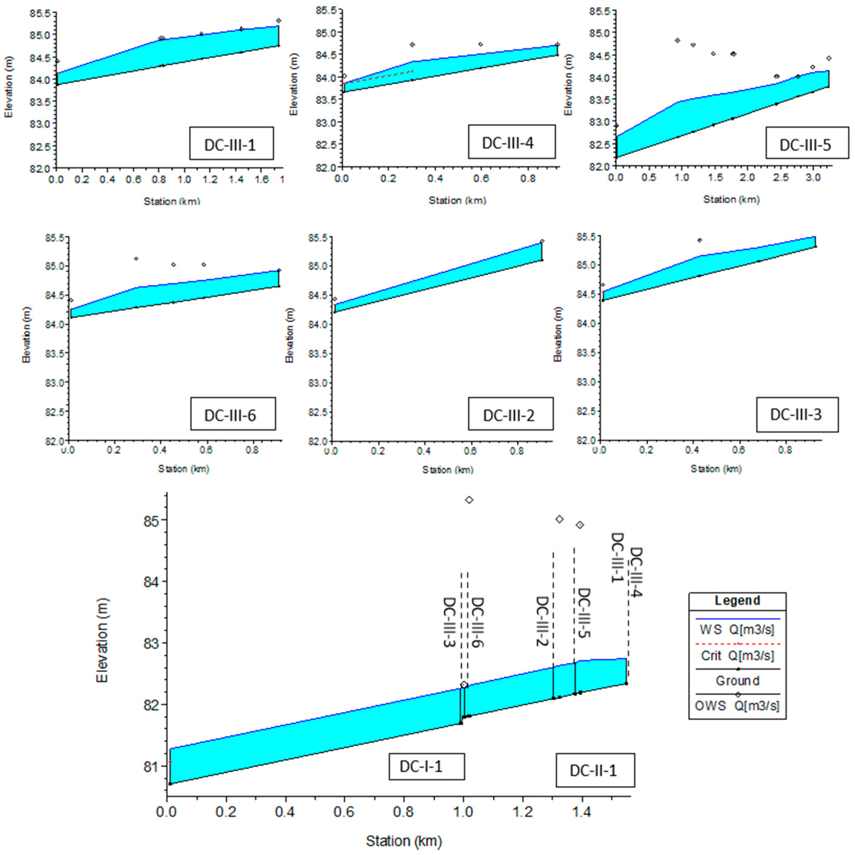
The objective of the drainage canal design is to create optimal geometry, capable of transporting the runoff, and lowering the ground water level for optimal crop yield while minimizing the canal dimensions at the same time. Therefore, lateral drain geometry is constrained by crop type, and optimization must start at the tertiary canal level, where objective is to archive the flow velocity within allowable tolerance (lower than the canal erosion critical velocity and higher than the velocity which would result in siltation) and water level lower than the water level in lateral drains. DrainCAN incorporates the restrictive water level in lateral drains as “observed water level” at the cross-sections of primary network canals. The observed water level is written into the imported steady flow file, thus enabling the optimization of the canals during design. The following figure (Figure 9) shows the tertiary canals in the network whose geometry was optimized using the aforementioned flow velocity and depth criteria. Variable parameters used for optimization of each canal are the invert elevation of the outlet and longitudinal slope. The cross-section geometry of the canal can also be used for optimization, but it was retained in this example because it reflects the constructed state.
In the profile plot, the observed water levels are indicated using diamond symbols. The adverse nature of the land topography of this agricultural study can be clearly seen on the DC-III-5, where the upstream lateral canals are located in the depression and impose restrictions on canal depth. This canal, in turn, influences the invert elevation of the secondary canal into which it inflows because the secondary canal invert must be lower or equal to the tertiary canal invert at its respective inflow location. For this reason, all other tertiary canals are significantly higher and have drops at the inflow locations. Drops are characterized by the flow acceleration at the outlet cross-section; in the steady flow regime, HEC-RAS uses a red label indicating critical velocity, i.e., Fr = 1. As can be seen, the inflow of all tertiary canals into secondary is achieved without backwater flow.
If backwater flow is to occur in tertiary canals, it would be clearly visible because DrainCAN calculates the normal depth for each canal and saves it as the observed water level for the most downstream cross-section. In order to avoid backwater flow in the canal, the water level at the outlet must be at/below the observed water level. For all tertiary canals, the water level at the outlet is below the normal depth level, meaning that outflow is unconstrained. For the given example, cross-sections are scarce and, therefore, the line of depression due to the accelerated flow is relatively long. If the user wants to calculate the water level profile with more accuracy, more cross-sections can be added in the CNS file without the need for additional runoff calculations.
The results of the HEC-RAS hydraulic model show that land topography significantly influences the flow characteristics of the tertiary canals. The longitudinal slope of the canals varies from 0.001 m/m (canal DC-III-4) to 0.00001 m/m (canals DC-III-5 and -6), reflecting the undulating topography of the eastern side of the land. On the other side, canals DC-III-1–3 have a more uniform slope, from 0.0005 to 0.0008 m/m. Total inflow in the canals is mostly dependent on their length, and it varies from 0.18 m3/s for the shortest canal in the network (DC-III-2) to 1.06 m3/s for the longest canal in the network (DC-III-5). Results obtained using the objective function for allowable velocity are uniform, and average flow velocity in the tertiary canals varies from 0.37 to 0.42 m/s, resulting in maximal flow depths from 0.23 (DC-III-2) m to 0.53 m (DC-III-5).
The starting point of the secondary canal DC-II-1 is at the junction of tertiary canals DC-III-1 and -4. It is 571 m long and collects water flow from all tertiary canals, resulting in the total flow at the outlet of 2.39 m3/s. Because of the depth of canal DC-III-5, canal DC-II-1 had to be lowered to match invert elevation at the inflow of DC-III-5 (station 0 + 385). To achieve the average velocity in the canal of 0.80 m/s, its slope is set as 0.00008 m/m, resulting in a maximum flow depth of 0.4 m. Since the secondary canal is deep, the criterion at its downstream end is to achieve normal depth, i.e., no backwater flow. From the HEC-RAS profile plot (Figure 9), it can be seen that at the junction of the primary and secondary canal, the flow depth coincides with the observed water level, indicating normal depth, and the continuity of canal geometry is therefore satisfied.
The DrainCAN function’s biggest advantage is fast generation of the HEC-RAS hydraulic model files from simple input files. It allows fast iteration of the canal design parameters of cross-sectional geometry, invert elevation, and longitudinal slope and the evaluation of introduced changes on the flow regime. The optimization variables introduced by DrainCAN—observed water levels for normal depth at canal outlet and for lateral drain location along the canal—allow for fast evaluation of effectiveness for each geometry. In the presented case study, it took 5 iterations to match the criteria of no backwater flow in tertiary canals, 4 iterations to achieve the required average velocity and 2 iterations to adjust for lateral drain elevation. The whole optimization process lasted approximately one hour. Another advantage of the DrainCAN function is the ability to recognize computational junctions in the model and adjust the canal geometry accordingly, without user input. This capability saves time as it alleviates the need for manually adjusting elevations, thus also reducing the possibility of erroneous data input in the process.
4. Conclusions
In this paper, we presented the MATLAB function DrainCAN for creating model geometry and flow data for input in HEC-RAS along with its advantages. The DrainCAN overlaps the corridor of the canals, forming the drainage network with scarce topographic data to derive compatible canal geometry to be used by HEC-RAS software. The advantage of the DrainCAN function is fast generation of the HEC-RAS input files for use in drainage canal optimization for small-scale projects that require fast hydraulic analysis. The potential for using the developed method also lies in the utilization of scarce input data, which is beneficial for projects that have a limited budget that does not allow for utilization of complex DTMs. The focus of the DrainCAN function is on optimization of the canal geometry in the design or restoration phase. To fully support the optimization process in geometry and flow data creation, DrainCAN incorporates optimization variables–it generates normal flow depth estimation and observed water levels in critical locations that need to be optimized. The developed function uses an .sdf file imported into HEC-RAS, which is a future-proof approach because it will be incorporated in future HEC-RAS versions.
Supplementary Materials
The following are available online at https://0-www-mdpi-com.brum.beds.ac.uk/article/10.3390/computation9050051/s1, MATLAB source code and working example (input files and HEC-RAS model).
Author Contributions
Conceptualization, G.G.; methodology, G.G.; software, G.G.; validation, G.G. and A.H.; formal analysis, G.G. and A.H.; investigation, A.H. and R.F.; resources, A.H.; data curation, G.G. and A.H.; writing—original draft preparation, G.G.; writing—review and editing, A.H. and R.F.; visualization, A.H. All authors have read and agreed to the published version of the manuscript.
Funding
This research received no external funding.
Informed Consent Statement
Not applicable.
Data Availability Statement
The data presented in this study are available in Supplementary Materials.
Acknowledgments
The authors would like to acknowledge the support of Faculty of Agriculture that has kindly provided us with the canal layout for the case study area.
Conflicts of Interest
The authors declare no conflict of interest.
References
- AQUASTAT. FAO AQUASTAT Database; AQUASTAT: Rome, Italy, 2020. [Google Scholar]
- FAO. The State of the World’s Land and Water Resources for Food and Agriculture (SOLAW)—Managing Systems at Risk; FAO: New York, NY, USA, 2011. [Google Scholar]
- Pereira, L.S.; Duarte, E.; Fragoso, R. Water Use: Recycling and Desalination for Agriculture. In Encyclopedia of Agriculture and Food Systems; Van Alfen, N.K., Ed.; Academic Press: Oxford, UK, 2014; pp. 407–424. [Google Scholar] [CrossRef]
- Ritzema, H. Main Drainage Systems; UNESCO-IHE: Wageningen, The Netherlands, 2014; p. 39. [Google Scholar]
- USDA. NRCS New Jersey Water Management Guide; Natural Resources Conservation Service: Somerset, NJ, USA, 2007; p. 165.
- Brunner, G.W.; CEIWR-HEC. HEC-RAS River Analysis System: User’s Manual Version 5.0; CPD-68; US Army Corps of Engineers—Hydrologic Engineering Center: Davis, CA, USA, 2016; p. 962. [Google Scholar]
- Agudelo Otálora, L.M.; Moscoso Barrera, W.D.; Paipa Galeano, L.A.; Mesa Sciarrotta, C. Comparison of physical models and artificial intelligence for prediction of flood levels. Tecnol. Cienc. Agua 2018, 9, 209–236. [Google Scholar] [CrossRef]
- Ahmad, H.F.; Alam, A.; Bhat, M.S.; Ahmad, S. One Dimensional Steady Flow Analysis Using HECRAS—A case of River Jhelum, Jammu and Kashmir. Eur. Sci. J. 2016, 12. [Google Scholar] [CrossRef]
- Marimin, N.A.; Mohammad Razi, M.A.; Ahmad, M.A.; Adnan, M.S.; Rahmat, S.N. HEC-RAS Hydraulic Model for Floodplain Area in Sembrong River. Int. J. Integr. Eng. 2018, 10. [Google Scholar] [CrossRef]
- Buta, C.; Mihai, G.; Stănescu, M. Flash floods simulation in a small drainage basin using HEC-RAS hydraulic model. Ovidius Univ. Ann. Ser. Civ. Eng. 2017, 19, 101–118. [Google Scholar] [CrossRef] [Green Version]
- Ezz, H. Integrating GIS and HEC-RAS to model Assiut plateau runoff. Egypt. J. Remote Sens. Space Sci. 2018, 21, 219–227. [Google Scholar] [CrossRef]
- Haliuc, A.; Frantiuc, A. A study case of Baranca drainage basin flash-floods using the hydrological model of Hec-Ras. Sci. Ann. Stefan Cel Mare Univ. Suceava. Geogr. Ser. 2012, 21. [Google Scholar] [CrossRef] [Green Version]
- Baky, A.A.; Zaman, A.M.; Khan, A.U. Managing Flood Flows for Crop Production Risk Management with Hydraulic and GIS Modeling: Case study of Agricultural Areas in Shariatpur. APCBEE Procedia 2012, 1, 318–324. [Google Scholar] [CrossRef] [Green Version]
- Raslan, A.M.; Riad, P.H.; Hagras, M.A. 1D hydraulic modelling of Bahr El-Baqar new channel for northwest Sinai reclamation project, Egypt. Ain Shams Eng. J. 2020, 11, 971–982. [Google Scholar] [CrossRef]
- Traore, V.B.; Bop, M.; Faye, M.; Malomar, G.; Gueye, E.H.O.; Sambou, H.; Dione, A.N.; Fall, S.; Diaw, A.T.; Sarr, J.; et al. Using of Hec-ras Model for Hydraulic Analysis of a River with Agricultural Vocation: A Case Study of the Kayanga River Basin, Senegal. Am. J. Water Resour. 2015, 3, 147–154. [Google Scholar] [CrossRef]
- Kiesel, J.; Schmalz, B.; Brown, G.L.; Fohrer, N. Application of a hydrological-hydraulic modelling cascade in lowlands for investigating water and sediment fluxes in catchment, channel and reach. J. Hydrol. Hydromech. 2013, 61, 334–346. [Google Scholar] [CrossRef] [Green Version]
- Sennaoui, F.; Benabdesselam, T.; Saihia, A. Use of modelling for the renovation of drainage channels—The case of the Bouteldja plain in northeastern Algeria. J. Water Land Dev. 2019, 43, 1–8. [Google Scholar] [CrossRef] [Green Version]
- WSU; UoW. A Study of Agricultural Drainage in the Puget Sound Lowlands to Determine Practices which Minimize Detrimental Effects on Salmonids: Final Report; Washington State University and University of Washington: Seattle, WA, USA, 2008. [Google Scholar]
- Nemati Kutenaee, M.; Shahnazari, A.; Fazoula, R.; Aghajanee Mazandarani, G.; Perraton, E. Effects of Caspian Sea water level fluctuations on existing drains. Casp. J. Environ. Sci. 2011, 9, 169–180. [Google Scholar]
- Xiao, L.; Chen, Z.; Zhou, F.; Hammouda, S.b.; Zhu, Y. Modeling of a Surface Flow Constructed Wetland Using the HEC-RAS and QUAL2K Models: A Comparative Analysis. Wetlands 2020, 40, 2235–2245. [Google Scholar] [CrossRef]
- Maharjan, L.; Shakya, N. Comparative Study of One Dimensional and Two Dimensional Steady Surface Flow Analysis. J. Adv. Coll. Eng. Manag. 2016, 2, 12–30. [Google Scholar] [CrossRef]
- ShahiriParsa, A.; Noori, M.; Heydari, M.; Rashidi, M. Floodplain Zoning Simulation by Using HEC-RAS and CCHE2D Models in the Sungai Maka River. Air Soil Water Res. 2016, 9. [Google Scholar] [CrossRef] [Green Version]
- Tate, E. Floodplain Mapping Using HEC-RAS and ArcView GIS; The University of Texas: Austin, TX, USA, 1999. [Google Scholar]
- Gee, D.M.; Brunner, G.W. Dam Break Flood Routing Using HEC-RAS and NWS-FLDWAV. In World Water and Environmental Resources Congress—Impacts of Global Climate Change; ASCE: Anchorage, AK, USA, 2005; pp. 1–9. [Google Scholar] [CrossRef]
- Rodriguez, L.B.; Cello, P.A.; Vionnet, C.A.; Goodrich, D. Fully conservative coupling of HEC-RAS with MODFLOW to simulate stream–aquifer interactions in a drainage basin. J. Hydrol. 2008, 353, 129–142. [Google Scholar] [CrossRef]
- Goodell, C. Breaking HEC-RAS Code—A User’s Guide to Automating HEC-RAS; H2ls: Portland, OR, USA, 2014; p. 247. [Google Scholar]
- Dysarz, T. Application of Python Scripting Techniques for Control and Automation of HEC-RAS Simulations. Water 2018, 10, 1382. [Google Scholar] [CrossRef] [Green Version]
- Saeed, M. Online Flood Forecasting Tool Using a Coupled Hydrological-Hydraulic Model: LARSIM & HEC-RAS—Case Study: Upper Main Catchment; Technical University of Munich: Munich, Germany, 2018; p. 65. [Google Scholar]
- Albo-Salih, H.H.K. Real-Time Operation of River-Reservoir Systems during Flood Conditions Using Optimization-Simulation Model. with One- and Two-Dimensional Modeling. Ph.D. Thesis, Arizona State University, Arizona, AZ, USA, 2019. [Google Scholar]
- Reinoso-Gordo, J.F.; Ibáñez, M.J.; Romero-Zaliz, R. Parallelizing drainage network algorithm using free software: Octave as a solution. Math. Comput. Simul. 2017, 137, 424–430. [Google Scholar] [CrossRef]
- Mokhtari, F.; Soltani, S.; Mousavi, S.A. Assessment of Flood Damage on Humans, Infrastructure, and Agriculture in the Ghamsar Watershed Using HEC-FIA Software. Nat. Hazards Rev. 2017, 18. [Google Scholar] [CrossRef]
- Gichamo, T.Z.; Popescu, I.; Jonoski, A.; Solomatine, D. River cross-section extraction from the ASTER global DEM for flood modeling. Environ. Model. Softw. 2012, 31, 37–46. [Google Scholar] [CrossRef]
- Tassew, B.G.; Belete, M.A.; Miegel, K. Application of HEC-HMS Model for Flow Simulation in the Lake Tana Basin: The Case of Gilgel Abay Catchment, Upper Blue Nile Basin, Ethiopia. Hydrology 2019, 6, 21. [Google Scholar] [CrossRef] [Green Version]
- Dijan, L. Estimating Flood Hazard on Agricultural Areas; University of Zagreb: Zagreb, Croatia, 2020. [Google Scholar]
- Wischounig, L. dxf2coord 2.0. MATLAB Central File Exchange. 2019. Available online: https://www.mathworks.com/matlabcentral/fileexchange/28791-dxf2coord-2-0 (accessed on 13 November 2019).
- Rees, I. distance_point_segment.py. GitHub. 2019. Available online: https://gist.github.com/irees/be5e56e7c9b16d78a351 (accessed on 13 November 2019).
- Rik. Point to Line Distance. GitHub. 2019. Available online: https://nl.mathworks.com/matlabcentral/fileexchange/64396-point-to-line-distance (accessed on 13 November 2019).
- Tiwari, H.; Das, P.; Bharti, A.K. MATLAB Programming Solution for Critical and Normal Depth in Trapezoidal Channels. Int. J. Eng. Res. Technol. 2012, 1, 1–3. [Google Scholar]
- Brunner, G.W.; CEIWR-HEC. HEC-RAS River Analysis System User’s Manual Version 4.1; US Army Corps of Engineers Institute for Water Resources—Hydrologic Engineering Center: Davis, CA, USA, 1995; p. 766. [Google Scholar]
- Leon, A.S.; Goodell, C. Controlling HEC-RAS using MATLAB. Environ. Model. Softw. 2016, 84, 339–348. [Google Scholar] [CrossRef] [Green Version]
- Tadić, T. Development of Coupled HEC-HMS/RAS for Runoff Modelling from Agricultural Land; University of Zagreb: Zagreb, Croatia, 2019. [Google Scholar]
Figure 1.
Typical scheme of drainage canal network.
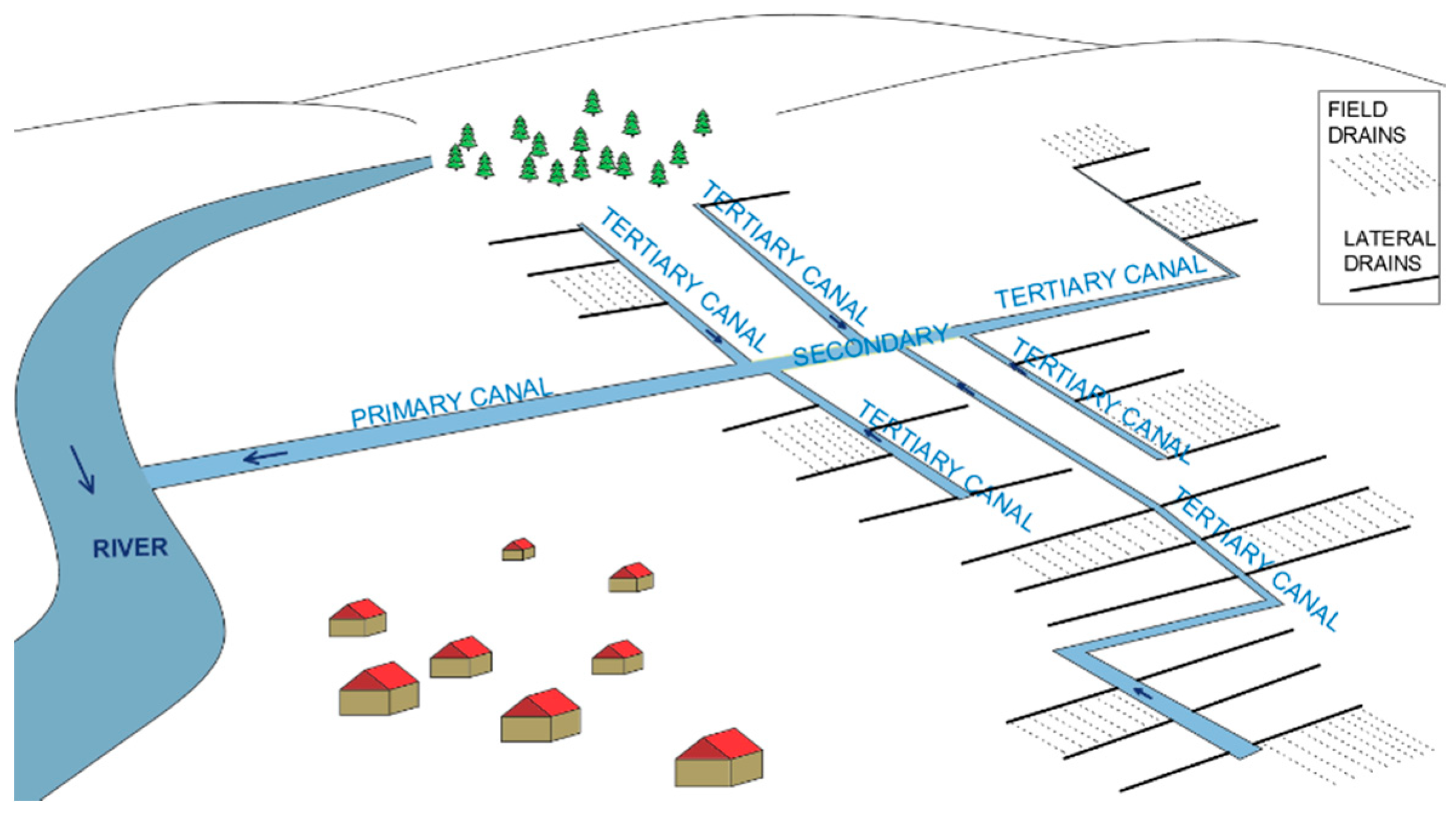
Figure 2.
Typical scheme of junctions on the canal network: outlet of field drains into lateral drain (left); formation of secondary canal on the junction of two tertiary canals (right).
Figure 2.
Typical scheme of junctions on the canal network: outlet of field drains into lateral drain (left); formation of secondary canal on the junction of two tertiary canals (right).

Figure 3.
Scheme of the drainage network prepared in AutoCAD for input into the function.

Figure 4.
Structure of the CGI input file (separate Excel worksheets are used for each canal in the network).
Figure 4.
Structure of the CGI input file (separate Excel worksheets are used for each canal in the network).

Figure 5.
Flow chart of the function block depicting the creation of cross-sectional geometry.

Figure 6.
Flow chart of the function block depicting the creation of hydraulic junctions (left) and creation of HEC-RAS input files (right).
Figure 6.
Flow chart of the function block depicting the creation of hydraulic junctions (left) and creation of HEC-RAS input files (right).

Figure 7.
Scheme of the existing drainage canal network: HEC-RAS model geometry (left); topographic map (right).
Figure 7.
Scheme of the existing drainage canal network: HEC-RAS model geometry (left); topographic map (right).
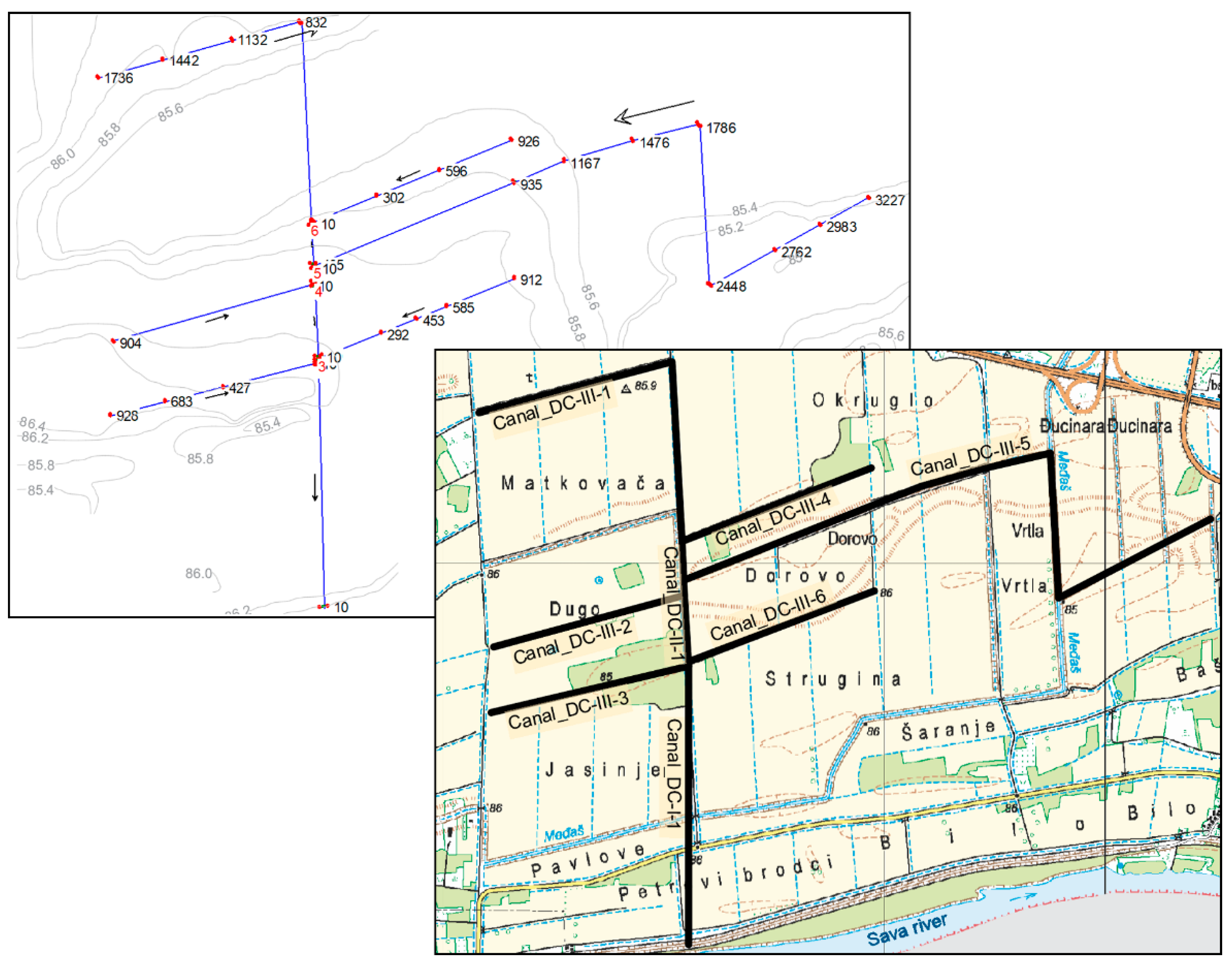
Figure 8.
Structure of estimated inflow data into primary drainage network (red labels highlight outflow from each tertiary canal; blue labels highlight the flow in the secondary canal at the confluences of tertiary canals).
Figure 8.
Structure of estimated inflow data into primary drainage network (red labels highlight outflow from each tertiary canal; blue labels highlight the flow in the secondary canal at the confluences of tertiary canals).

Figure 9.
HEC-RAS profile plot of primary, secondary, and tertiary drains with optimization variables (normal depth at confluence and lateral drain height along the canal, diamond symbols).
Figure 9.
HEC-RAS profile plot of primary, secondary, and tertiary drains with optimization variables (normal depth at confluence and lateral drain height along the canal, diamond symbols).
Publisher’s Note: MDPI stays neutral with regard to jurisdictional claims in published maps and institutional affiliations. |
© 2021 by the authors. Licensee MDPI, Basel, Switzerland. This article is an open access article distributed under the terms and conditions of the Creative Commons Attribution (CC BY) license (https://creativecommons.org/licenses/by/4.0/).
Share and Cite
MDPI and ACS Style
Gilja, G.; Harasti, A.; Fliszar, R. DrainCAN—A MATLAB Function for Generation of a HEC-RAS-Compatible Drainage Canal Network Model. Computation 2021, 9, 51. https://0-doi-org.brum.beds.ac.uk/10.3390/computation9050051
AMA Style
Gilja G, Harasti A, Fliszar R. DrainCAN—A MATLAB Function for Generation of a HEC-RAS-Compatible Drainage Canal Network Model. Computation. 2021; 9(5):51. https://0-doi-org.brum.beds.ac.uk/10.3390/computation9050051
Chicago/Turabian StyleGilja, Gordon, Antonija Harasti, and Robert Fliszar. 2021. "DrainCAN—A MATLAB Function for Generation of a HEC-RAS-Compatible Drainage Canal Network Model" Computation 9, no. 5: 51. https://0-doi-org.brum.beds.ac.uk/10.3390/computation9050051
Note that from the first issue of 2016, this journal uses article numbers instead of page numbers. See further details here.