
Predicting Interfacial Thermal Resistance by Ensemble Learning
by
 , ,
, ,
Mingguang Chen
1,*, 
Junzhu Li
1,
Bo Tian
1,
Yas Mohammed Al-Hadeethi
2,
Bassim Arkook
2,3,
Xiaojuan Tian
4,* and
Xixiang Zhang
1,* 1
Physical Science and Engineering Division, King Abdullah University of Science and Technology (KAUST), Thuwal 23955-6900, Saudi Arabia
2
Department of Physics, King Abdulaziz University, Jeddah, Makkah 21589, Saudi Arabia
3
Department of Physics and Astronomy, University of California, Riverside, CA 92507, USA
4
Department of Chemical Engineering, China University of Petroleum, Beijing 102249, China
*
Authors to whom correspondence should be addressed.
Computation 2021, 9(8), 87; https://0-doi-org.brum.beds.ac.uk/10.3390/computation9080087
Submission received: 26 June 2021
/
Revised: 22 July 2021
/
Accepted: 24 July 2021
/
Published: 2 August 2021
(This article belongs to the Section Computational Engineering)
Abstract
:Interfacial thermal resistance (ITR) plays a critical role in the thermal properties of a variety of material systems. Accurate and reliable ITR prediction is vital in the structure design and thermal management of nanodevices, aircraft, buildings, etc. However, because ITR is affected by dozens of factors, traditional models have difficulty predicting it. To address this high-dimensional problem, we employ machine learning and deep learning algorithms in this work. First, exploratory data analysis and data visualization were performed on the raw data to obtain a comprehensive picture of the objects. Second, XGBoost was chosen to demonstrate the significance of various descriptors in ITR prediction. Following that, the top 20 descriptors with the highest importance scores were chosen except for fdensity, fmass, and smass, to build concise models based on XGBoost, Kernel Ridge Regression, and deep neural network algorithms. Finally, ensemble learning was used to combine all three models and predict high melting points, high ITR material systems for spacecraft, automotive, building insulation, etc. The predicted ITR of the Pb/diamond high melting point material system was consistent with the experimental value reported in the literature, while the other predicted material systems provide valuable guidelines for experimentalists and engineers searching for high melting point, high ITR material systems.
1. Introduction
Interfacial thermal resistance (ITR) is a property that measures an interface’s resistance to thermal flow [1,2,3]. When thermal flux is applied across an interface, ITR causes a finite temperature discontinuity. Low ITR is technologically important for heat dissipation in integrated circuits [4], whereas high ITR is critical for engine turbine protection [5,6]. The growing interest in space exploration necessitates developing special material systems that can withstand high temperatures and have high ITR. A reliable and accurate prediction of ITR is thus critical for the design of materials with desired properties. However, ITR is affected by a wide range of factors, including melting point, film thickness, material density, heat capacity, electronegativity, binding energy, and temperature [7,8]. Furthermore, for nanodevices, quantum effects must be considered [9]. As a result, ITR prediction is a high-dimensional problem that cannot be solved ideally using traditional methods.
The traditional representative models for predicting ITR are the acoustic mismatch model (AMM), diffuse mismatch model (DMM) [10], scattering-mediated acoustic mismatch model (SMAMM) [11], and molecular dynamics simulation (MD) [12]. To some extent, these models all have simplified assumptions, which limit the prediction to specific scenarios. Briefly, the AMM model is based on the idea that ITR is caused by an acoustic impedance mismatch between two materials. Other factors, such as phonon scattering, geometry, and chemical bonds, are ignored, resulting in AMM working well only at low temperatures and underestimating ITR at high temperatures [13]. The DMM is proposed as a supplement to AMM. It assumes complete phonon scattering at the interface, resulting in the overestimation of ITR, particularly at low temperatures [10]. The SMAMM improves the AMM model by incorporating phonon scattering and achieves reasonable ITR prediction over a wider temperature range. However, its accuracy is still limited due to the omission of other factors influencing ITR. As an atomic-level simulation, MD simulation considers chemical bonds, defects, and atomic species at interfaces and can outperform AMM, DMM, and SMAMM models [12]. However, because inelastic quantum scattering is difficult to capture in MD simulation, it is challenging to integrate quantum effects [14]. In addition, MD simulation is computationally expensive, preventing its applications to complex material systems. The rise of machine learning in the last decade has enabled the solution of high-dimensional problems. The goal of machine learning is to automatically discover the underlying pattern by training models on given datasets. The Xu group predicted ITR using classical machine learning methods (LSBoost, support vector machines, and Gaussian process regression) and achieved higher prediction accuracy than traditional AMM and DMM models [7,8]. Table 1 summarizes the advantages and disadvantages of machine learning models in ITR prediction when compared to traditional AMM, DMM, and SMAMM models, and MD simulations.
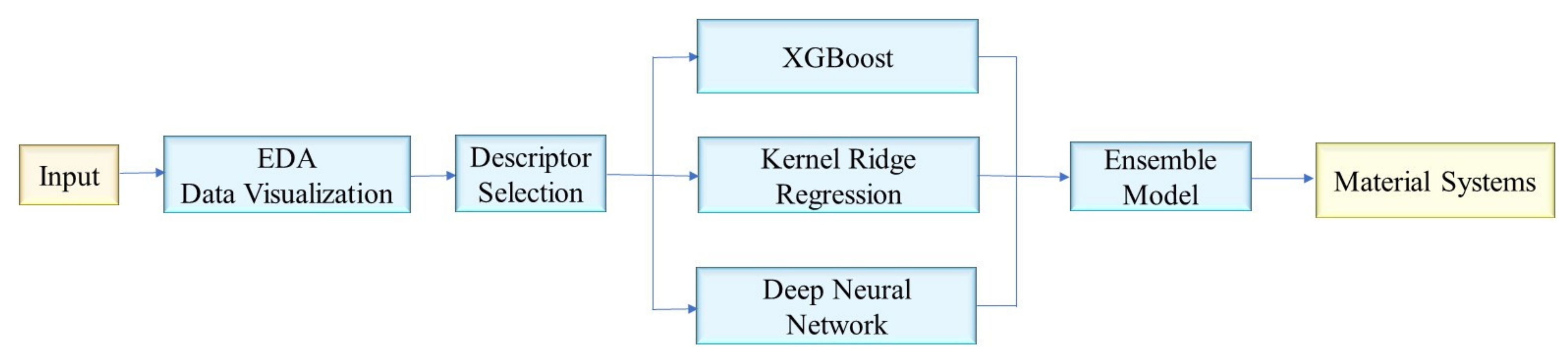
In general, machine learning models are more reliable when trained on large datasets [18,19]. However, the available ITR dataset from the literature is relatively small (692 instances) [7,8]. In this case, the corresponding machine learning models are prone to overfitting, thereby reducing prediction accuracy and robustness. In this work, we used ensemble learning to reduce the overfitting of machine learning models and achieve a robust and precise ITR prediction, as illustrated in Figure 1. First, exploratory data analysis (EDA) and data visualization were performed on the raw data to obtain a comprehensive view of the dataset. The correlations between training descriptors and target ITR values were used to select descriptors. Second, the XGBoost (XGB) algorithm was chosen to create an interpretable XGB model and demonstrate the significance of various descriptors in ITR prediction. Following that, the top 20 descriptors with the highest importance scores were chosen, except for fdensity, fmass, and smass, to build concise models using XGBoost, Kernel Ridge Regression, and deep neural networks. An ensemble model was created by combining these three models. Finally, over 80,000 material systems were constructed and used as test data for ITR predictions. The top 40 material systems with melting points higher than 600 K predicted by our ensemble model were reported.
2. Methods
2.1. Dataset Collection
The dataset(“training dataset for ITR prediction.xlsx” and “descriptor dataset.xlsx”) was collected from the literature, organized by the Xu group [7,8], and can be downloaded directly from: https://0-doi-org.brum.beds.ac.uk/10.5281/zenodo.3564173 (accessed on 28 July 2021).
2.2. Dataset Preprocessing
Descriptors were scaled before being fed into models. According to the distribution of descriptors, the min–max scale and standard scale were used. The min–max scaler transforms the descriptors fthick, fmelt, fdensity, sdensity, fAC1x, fAC1y, fAC2x, fAC2y, fIPc, fIPa, smelt, sAC1x, sAC1y, sAC2x, sAC2y, sIPc, and sIPa. T, fmass, fEb, sEb, and smass are the descriptors transformed by the standard scaler. Table S1 summarizes the meaning of each descriptor’s abbreviation.
Material systems were constructed using the “descriptor dataset.” The corresponding python codes’ material system construction for ITR prediction can be downloaded directly from: https://github.com/pacificknight/Ensemble-learning-for-ITR-prediction (accessed on 28 July 2021).
2.2.1. XGBoost
The XGB is a gradient boosting library implementation designed for high speed and accuracy in solving many data science problems [20]. Another advantage of XGB is that obtaining importance scores for each descriptor after the boosted trees are constructed is relatively straightforward. Importance scores indicate a descriptor’s contribution to the final prediction and serve as guidelines for descriptor selection. The greater a descriptor’s importance score, the more it contributes to the final prediction. The training time for the XGB model with the selected descriptors is 0.16 s.
2.2.2. Kernel Ridge Regression
The KRR was chosen because it is a well-known machine learning method. It applies the powerful idea of support vector machines to regression. KRR improves computational efficiency by combining ridge regression with the “kernel trick” and extending ridge regression to the nonlinear case [21,22,23,24]. In this work, the radial basis function was used as the kernel. The training time for the KRR model with selected descriptors is 0.045 s.
2.2.3. Deep Neural Network
A deep neural network (DNN) is an artificial neural network with more than three hidden layers between the input and output layers. The DNNs are feedforward networks suitable for modeling complex nonlinear relationships [25,26,27]. There are several reasons to use DNN. First, DNN differs from traditional machine learning methods. It represents cutting-edge deep learning technology. Second, we expected to use DNN to capture potential patterns that may be ignored by traditional machine learning models in ITR predictions. Lastly, DNN can eliminate feature engineering and generate layered structures that eliminate representational redundancy. The parameter optimization of DNN is based on backpropagation. DNN is prone to overfitting; thus, regularization is widely adopted in DNN to penalize overfitting and make the model more robust and reliable [27,28]. A DNN with three hidden layers was constructed. From the first hidden layer to the last hidden layer, the neuron numbers were 64, 128, and 64, respectively. Root mean squared error (RMSE) was used as the loss function. Adam optimizer was employed with a weight decay of 5 × 10⁻⁵, a learning rate of 3 × 10⁻⁴. The training epochs were 15,000. R2 and RMSE were used to evaluate the model performance. First, batch normalization was performed on the input data using the equation below.
where and are the mean and standard deviation, respectively. The purpose of batch normalization is to accelerate DNN training by reducing internal covariate shifts [29]. The data was then transformed from 17 to 64 dimensions using a linear transformation and the Relu activation function, and nonlinear relationships were introduced into the model. Following that, the data was passed through the hidden layers. Dropout layers with a drop rate of 0.25 were added to each hidden layer after batch normalization and before linear transformation as a regularization method to reduce overfitting. Dropout refers to the process of randomly removing a percentage of neurons from our DNN during the training process [30]. By this act, the final ITR results will no longer depend on specific neurons, making the DNN model more robust and reliable. Furthermore, our DNN was trained with Adam optimizer at a decay weight rate of 5 × 10⁻⁵. Weight decay is another method of regularization [31]. Weight decay is based on the idea that neural networks with smaller weights are less likely to overfit. Given that large prediction error in ITR is misleading to materials design, we chose MSE over mean absolute error as the criterion in our DNN, which penalized large error more heavily. The DNN model with selected descriptors takes 434 s to train.
2.2.4. Ensemble Model
The XGB, KRR, and DNN models were used as base estimators. The ensemble model is built by combining all of the models used in the ITR prediction process to predict low variance, high accuracy, less feature noise, and bias. The aggregating method adopted is averaging. As a result, the final prediction was made by averaging the predicting results of XGB, KRR, and DNN models.
Even though the ITR has insignificant temperature dependence above room temperature in the training example, when constructing the test samples, the temperature used to predict high melting point ITR was set to be 600 K.
2.3. Algorithm Evaluation
The R2 score and RMSE were used to evaluate the model performances. The R2 score is also known as the coefficient of determination in statistics, and it measures how well-observed outcomes are replicated by the model [32]. The R2 score has a range of 0–1. The closer the R2 score is to 1, the better the model performance. The RMSE is often used to measure the difference between a model’s real and the predicted value [33]. For the same dataset, the smaller the RMSE, the better the model’s performance.
In statistics, R2 is calculated by
The RMSE is given by
where and are numbers of data instances, real ITR, predicted ITR, and averaged real ITR values, respectively.
3. Results and Discussion
3.1. Descriptor Selection
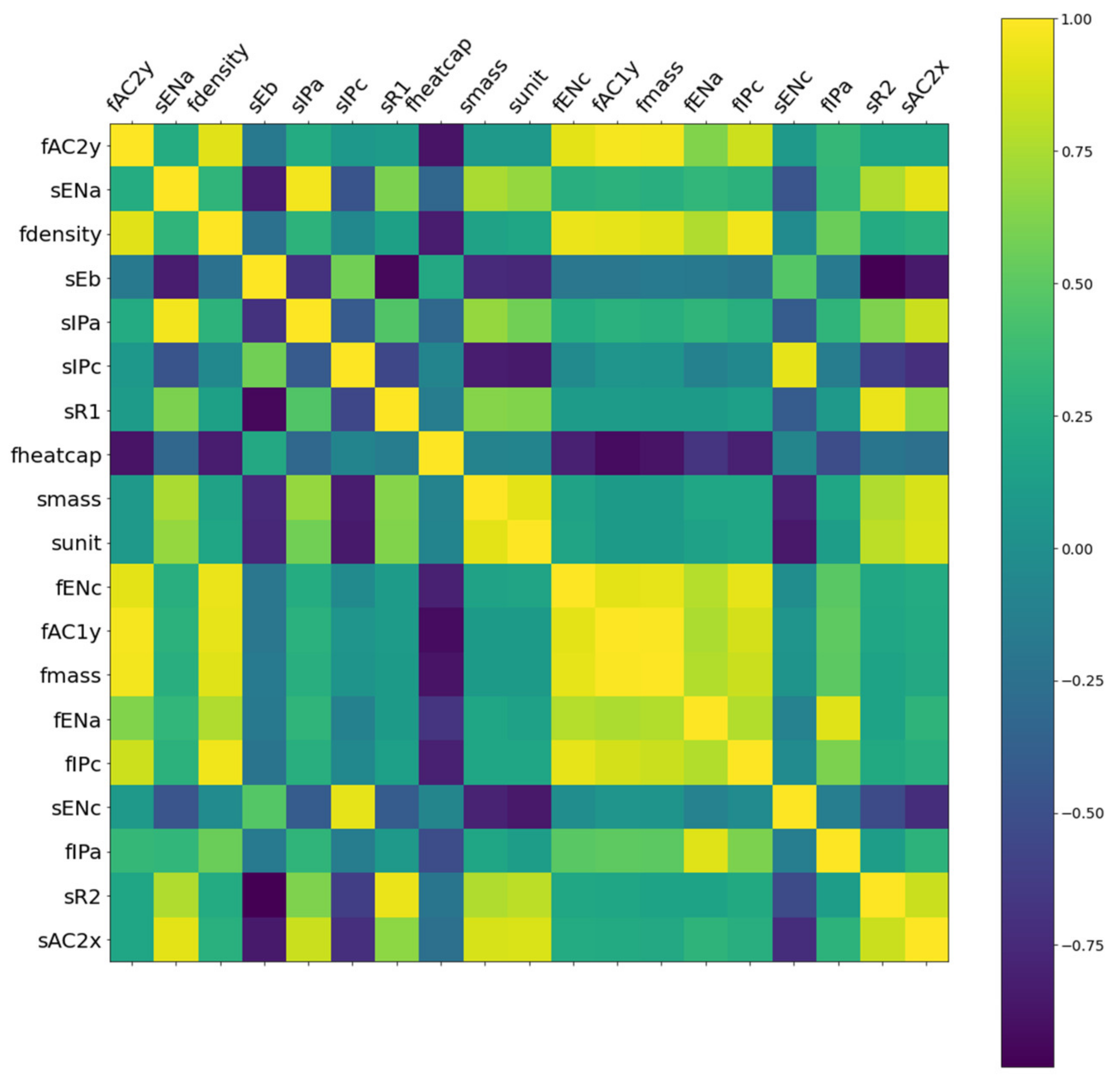
The EDA is a statistical approach for analyzing and summarizing datasets and their characteristics [34]. First, the Pearson heatmap of correlations between all 35 descriptors was calculated and plotted in Figure S1. The heatmap is diagonally symmetric because the correlation between descriptor A and descriptor B is equal to the correlation between descriptor B and descriptor A. The correlation between all 35 descriptors ranges from −1 to 1, with some descriptors having a high correlation with one another (yellow or dark areas). Figure 2 shows a heatmap of descriptors with absolute correlation values greater than 0.9. These highly correlated descriptors suggest that descriptor dimensions can be significantly reduced without negatively impacting model performance. For example, fmass has a correlation value of 0.9 with fdensity consistent with the two descriptors’ physical correlation. As a result, descriptor selection is required to reduce descriptor dimensions for a quick and reliable prediction. Second, the Pearson correlation coefficient between each descriptor and the target ITR was investigated, as shown in Figure 3. Descriptors such as funit, fmass, fAC2y, and fAC1y have a strong positive correlation with ITR, whereas fheatcap, sheatcap, fmelt, and T demonstrate a strong negative correlation with ITR. It is important to note that descriptor selection should not be based solely on the absolute value of descriptor correlations with ITR. For example, if we build models using high correlation descriptors like fmass, fAC2y, and fAC1y, the prediction results will be inaccurate. Because descriptors fAC2y and fAC1y have a high correlation with descriptor fmass, as shown in Figure 2, models with all three descriptors are not expected to outperform models containing only one of the three descriptors. In light of this, we chose descriptor based not only on the importance scores of each descriptor provided by the XGB model but also on the Pearson correlation coefficients.
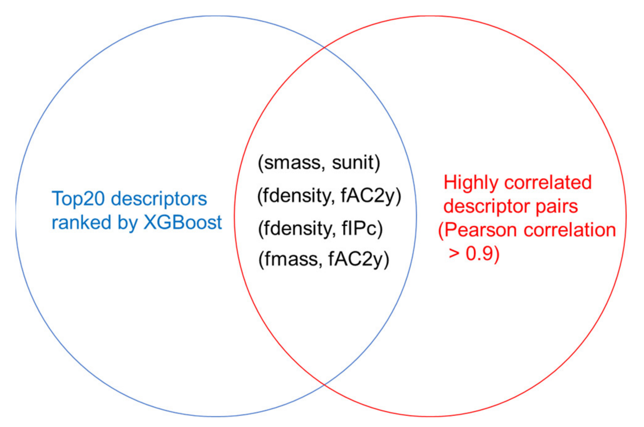
First, an XGB model with all 35 descriptors was built, and the corresponding parameters were optimized. The test dataset had an R2 score of 0.88 and an RMSE of 9.44. To better understand the contributions of each descriptor, the ranked descriptor importance of all 35 descriptors was given in Figure S2. It indicates that the binding energy, volume per formula unit, melting point, density, heat capacity, and temperature, among other factors, play a significant role in predicting ITR. For example, binding energy and melting point can influence phonon transport; volume per formula unit and density can influence the Debye cutoff frequency; [8] and temperature can influence ITR directly through heat capacity and phonon distribution [35]. However, some of the descriptors are highly correlated with one another and thus redundant for ITR prediction. In addition, it is difficult to collect all of the descriptor data in practice, which dictates descriptor selection. Figure 4 shows the descriptor selection procedures. First, the top 20 descriptors with the highest importance scores were selected. Then, within the top 20 descriptors (fdensity, fmass, and smass), duplicated descriptors were removed, yielding 17 relatively independent dominating descriptors.
3.2. Model Performance
In this section, we trained and evaluated the performance of a new XGB model with the 17 descriptors obtained from the preceding section. The R2 score and RMSE obtained for the test dataset were 0.87 and 10.00, respectively, comparable to the XGB model trained with all 35 descriptors. This indicates that we have extracted all necessary descriptors to build reliable and concise machine learning models. The KRR and DNN models were also trained with the training data and evaluated with the test data. Table 2 summarizes the predictive performance of all three models evaluated by R2 and RMSE. After descriptor selection, all three models maintained high predictive performance, resulting in concise and accurate models.
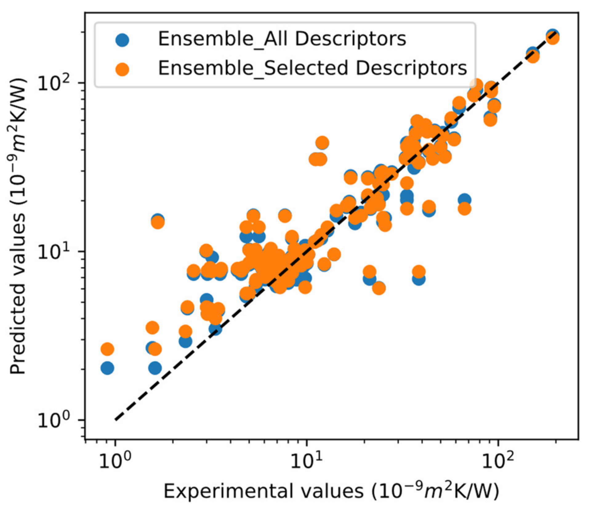
According to the no free lunch theorem, there is no universally best machine learning algorithm. Almost all machine learning algorithms are based on few assumptions (learning bias) about the relationship between descriptors and targets. Some algorithms perform better on certain datasets than others, while some datasets will not be modeled effectively by a given algorithm [36]. Ensemble learning combines the benefits of various algorithms to achieve higher predictive accuracy than individual algorithms [37]. Common types of ensembles include bootstrap aggregating [38], boosting [39], Bayesian model averaging [40], Bayesian model combination [41], Bucket of models [42], and stacking and averaging etc. [43,44]. As the raw dataset for ITR prediction is small, our individual models are more or less overfitted. Ensemble averaging has been demonstrated to reduce overfitting to some extent and make predictions more robust. As a result, we averaged the prediction results of all our models (XGB, KRR, and DNN models) to make a final ITR prediction, leading to higher R and lower RMSE than any individual model shown in Table 1, indicating better predictive performance. Figure 5 shows the experimental ITR versus the predicted ITR values of the ensemble model. The blue dots represent values predicted with all descriptors and the orange dots represent results predicted with selected descriptors. As we can see, the majority of the blue and orange dots overlapped and is located near the black diagonal dash line. Similarly, the correlations between experimental ITR and predicted ITR forecasted by individual models (XGB, KRR, and DNN) before and after descriptor selection were given in Figures S3–S5. The high overlap between orange and blue dots indicates that we have selected all necessary descriptors, and built a concise ensemble model with improved predictive performances.
The concise ensemble model was then used to search high melting point, high ITR material systems. To benchmark the prediction performance of our ensemble model, the predicted top 20 materials systems with high ITR was listed in Table S2. Bi/Diamond, Bi/graphite, Bi/P, Bi/B, Bi/BN, and Bi/BeO systems were also predicted by other groups in the literature, indicating the effectiveness of our ensemble model. To predict high melting points, high ITR material systems, material systems with melting points higher than 600 K were filtered and ranked based on the ITR values. The top 20 high melting points and high ITR material systems predicted by the ensemble model are listed in Table 3. The top predicted material systems are mainly composed of carbon-based substrates, such as diamond, graphite, and graphene. Carbon materials have long been the focus of scientific and industrial communities due to their exceptional electrical, thermal, optical, and mechanical properties. Diamond, graphite, graphene, and carbon nanotubes, for example, have high melting points due to C–C covalent bonds.
Furthermore, as synthesis technologies evolve, graphite and graphene can be economically produced on a large scale. As a result, we encourage experimentalists to follow our predictions and explore high melting points, high ITR material systems for practical applications such as spacecraft, automobiles, building insulation, etc. Some of the predicted material systems have been experimentally validated, according to reports in the literature. For example, it has been reported that a Pb/Diamond material system has a very low interface thermal conductance of 25 MW/m2K [45], corresponding to very high ITR 40 (10−9 m2K/W). This indicates that our model has a high prediction accuracy. Although some material systems, such as CdTe/Diamond, have been explored for solar cells [46], their ITRs are yet to be measured and reported.
4. Conclusions
In this study, using ensemble learning, we predicted ITR in a robust and reliable approach. The EDA and data visualization were conducted to analyze the raw dataset, summarize its characteristics, and provide guidance for descriptor engineering. The XGB model’s importance scores and Pearson coefficients of descriptors were employed for descriptor selection and dimension reduction. To create concise models, 17 out of 35 descriptors were chosen. For ITR prediction, an ensemble model based on the XGB, KRR, and DNN algorithms was developed. The predicted ITR values were used to identify and rank material systems with high melting points and high ITR. The ITR of the Pb/Diamond system predicted by our ensemble model was highly consistent with the experimental value reported in the literature, indicating the high prediction performance of our ensemble model. The predicted material systems provide effective guidelines and significantly reduce the effort required by experimentalists and engineers to search for high melting, high ITR material systems.
The current data used for training models have several limitations. First, the data set is small, and it cannot cover all of the material systems required for training. Second, the data contains only a small fraction (2.9%) of two-dimensional material systems, which must be improved by combining more data from experiments.
Our future work will be focused on developing a database for ITR data from various material systems and collecting additional ITR data from recent literature and experiments. Furthermore, we intend to investigate multicomponent (>2) high melting points, high ITR material systems by synthesizing corresponding nanomaterial compounds. For example, we can synthesize PtTe, PdTe, and graphite nanomaterials separately, and uniformly combine them to produce PtTe/PdTe/graphite nano compounds for practical applications.
Supplementary Materials
The following are available online at https://0-www-mdpi-com.brum.beds.ac.uk/article/10.3390/computation9080087/s1, Figure S1: Pearson correlation coefficient map between all 35 descriptors in the raw dataset. Figure S2: Rank of Descriptors based on importance score provided by XGB model. Figure S3: Correlation between the experimental values and values predicted by XGB model with all descriptors (blue dots) and selected descriptors (orange dots). Figure S4: Correlation between the experimental values and values predicted by KRR model with all descriptors (blue dots) and selected descriptors (orange dots). Figure S5: Correlation between the experimental values and values predicted by DNN model with all descriptors (blue dots) and selected descriptors (orange dots). Table S1: Abbreviations of descriptors and the target explored in this work. Table S2: Top 20 material systems with high ITR predicted by ensemble model.
Author Contributions
Conceptualization, M.C., X.T., and X.Z.; Formal analysis, J.L. and B.T.; Investigation, Y.M.A.-H. and B.A.; Writing–original draft, M.C. and X.T.; Writing–review & editing, X.Z. All authors have read and agreed to the published version of the manuscript.
Funding
The work reported was funded by the King Abdullah University of Science and Technology (KAUST), Office of Sponsored Research (OSR), under the Award Nos. CRF-2018-3717-CRG7 and CRF-2015-2996 -CRG5, and by the National Natural Science Foundation of China under Award No. 21808240.
Data Availability Statement
The data presented in this study are available on request from the corresponding author. The data are not publicly available due to privacy.
Conflicts of Interest
There are no conflicts of interest to declare.
References
- Nan, C.W.; Birringer, R.; Clarke, D.R.; Gleiter, H. Effective thermal conductivity of particulate composites with interfacial thermal resistance. J. Appl. Phys. 1997, 81, 6692–6699. [Google Scholar] [CrossRef]
- Zhong, H.; Lukes, J.R. Interfacial thermal resistance between carbon nanotubes: Molecular dynamics simulations and analytical thermal modeling. Phys. Rev. B 2006, 74, 125403. [Google Scholar] [CrossRef] [Green Version]
- Hu, L.; Desai, T.; Keblinski, P. Determination of interfacial thermal resistance at the nanoscale. Phys. Rev. B 2011, 83, 195423. [Google Scholar] [CrossRef] [Green Version]
- Chung, C.; Lin, H.; Wan, W.; Yang, M.T.; Liu, C. Thermal SPICE modeling of FinFET and BEOL considering frequency-dependent transient response, 3-D heat flow, boundary/alloy scattering, and interfacial thermal resistance. IEEE Trans. Electron. Devices 2019, 66, 2710–2714. [Google Scholar] [CrossRef]
- Clarke, D.R.; Oechsner, M.; Padture, N.P. Thermal-barrier coatings for more efficient gas-turbine engines. MRS Bull. 2012, 37, 891–898. [Google Scholar] [CrossRef] [Green Version]
- Drexler, J.M.; Gledhill, A.D.; Shinoda, K.; Vasiliev, A.L.; Reddy, K.M.; Sampath, S.; Padture, N.P. Jet engine coatings for resisting volcanic ash damage. Adv. Mater. 2011, 23, 2419–2424. [Google Scholar] [CrossRef]
- Wu, Y.; Fang, L.; Xu, Y. Predicting interfacial thermal resistance by machine learning. Npj Comput. Mater. 2019, 5, 1–8. [Google Scholar] [CrossRef] [Green Version]
- Zhan, T.; Fang, L.; Xu, Y. Prediction of thermal boundary resistance by the machine learning method. Sci. Rep. 2017, 7, 1–9. [Google Scholar] [CrossRef] [PubMed] [Green Version]
- Shenogin, S.; Xue, L.; Ozisik, R.; Keblinski, P.; Cahill, D.G. Role of thermal boundary resistance on the heat flow in carbon-nanotube composites. J. Appl. Phys. 2004, 95, 8136–8144. [Google Scholar] [CrossRef]
- Swartz, E.T.; Pohl, R.O. Thermal resistance at interfaces. Appl. Phys. Lett. 1987, 51, 2200–2202. [Google Scholar] [CrossRef]
- Prasher, R.S.; Phelan, P.E. A scattering-mediated acoustic mismatch model for the prediction of thermal boundary resistance. J. Heat Transf. 2001, 123, 105–112. [Google Scholar] [CrossRef]
- Hu, M.; Shenogin, S.; Keblinski, P. Molecular dynamics simulation of interfacial thermal conductance between silicon and amorphous polyethylene. Appl. Phys. Lett. 2007, 91, 241910. [Google Scholar] [CrossRef]
- Little, W.A. The transport of heat between dissimilar solids at low temperatures. Can. J. Phys. 1959, 37, 334–349. [Google Scholar] [CrossRef]
- Zhou, H.; Zhang, G. General theories and features of interfacial thermal transport. Chin. Phys. B 2018, 27, 034401. [Google Scholar] [CrossRef] [Green Version]
- Prasher, R. Acoustic mismatch model for thermal contact resistance of van der Waals contacts. App. Phys. Lett. 2009, 94, 041905. [Google Scholar] [CrossRef] [Green Version]
- Reddy, P.; Castelino, K.; Majumdar, A. Diffuse mismatch model of thermal boundary conductance using exact phonon dispersion. Appl. Phys. Lett. 2005, 87, 211908. [Google Scholar] [CrossRef]
- Zhang, J.; Hong, Y.; Liu, M.; Yue, Y.; Xiong, Q.; Lorenzini, G. Molecular dynamics simulation of the interfacial thermal resistance between phosphorene and silicon substrate. Int. J. Heat Mass Transf. 2017, 104, 871–877. [Google Scholar] [CrossRef]
- Liang, G.; Mo, H.; Wang, Z.; Dong, C.; Wang, J. Joint deep recurrent network embedding and edge flow estimation. In Proceedings of the International Conference on Intelligent Computing, Bari, Italy, 2–5 October 2020; pp. 467–475. [Google Scholar]
- Liang, G.; Mo, H.; Qiao, Y.; Wang, C.; Wang, J. Paying deep attention to both neighbors and multiple tasks. In Proceedings of the International Conference on Intelligent Computing, Bari, Italy, 2–5 October 2020; pp. 140–149. [Google Scholar]
- Chen, T.; Guestrin, C. Xgboost: A scalable tree boosting system. In Proceedings of the 22nd ACM SIGKDD International Conference on Knowledge Discovery and Data Mining, San Francisco, CA, USA, 13–17 August 2016; pp. 785–794. [Google Scholar]
- Schölkopf, B.; Smola, A.; Müller, K.R. Nonlinear component analysis as a kernel eigenvalue problem. Neural Comput. 1998, 10, 1299–1319. [Google Scholar] [CrossRef] [Green Version]
- Yu, H.; Kim, S. SVM tutorial-classification, regression and ranking. Handb. Nat. Comput. 2012, 1, 479–506. [Google Scholar]
- Zhang, Y.; Duchi, J.; Wainwright, M. Divide and conquer kernel ridge regression. In Proceedings of the Conference on Learning Theory, Princeton, NJ, USA, 12–14 June 2013; pp. 592–617. [Google Scholar]
- An, S.; Liu, W.; Venkatesh, S. Face recognition using kernel ridge regression. In Proceedings of the 2007 IEEE Conference on Computer Vision and Pattern Recognition, Minneapolis, MN, USA, 17–22 June 2007; pp. 1–7. [Google Scholar]
- Deng, L.; Hinton, G.; Kingsbury, B. New types of deep neural network learning for speech recognition and related applications: An overview. In Proceedings of the 2013 IEEE International Conference on Acoustics, Speech and Signal Processing, Vancouver, BC, Canada, 26–31 May 2013; pp. 8599–8603. [Google Scholar]
- Hinton, G.; Deng, L.; Yu, D.; Dahl, G.E.; Mohamed, A.; Jaitly, N.; Senior, A.; Vanhoucke, V.; Nguyen, P.; Sainath, T.N. Deep neural networks for acoustic modeling in speech recognition: The shared views of four research groups. IEEE Signal. Process. Mag. 2012, 29, 82–97. [Google Scholar] [CrossRef]
- Ciregan, D.; Meier, U.; Schmidhuber, J. Multi-column deep neural networks for image classification. In Proceedings of the 2012 IEEE Conference on Computer Vision and Pattern Recognition, Providence, RI, USA, 16–21 June 2012; pp. 3642–3649. [Google Scholar]
- Jiang, Y.; Wu, Z.; Wang, J.; Xue, X.; Chang, S. Exploiting feature and class relationships in video categorization with regularized deep neural networks. IEEE Trans. Pattern Anal. Mach. Intell. 2017, 40, 352–364. [Google Scholar] [CrossRef] [PubMed]
- Santurkar, S.; Tsipras, D.; Ilyas, A.; Madry, A. How does batch normalization help optimization? arXiv 2018, arXiv:1805.11604. [Google Scholar]
- Srivastava, N.; Hinton, G.; Krizhevsky, A.; Sutskever, I.; Salakhutdinov, R. Dropout: A simple way to prevent neural networks from overfitting. J. Mach. Learn. Res. 2014, 15, 1929–1958. [Google Scholar]
- Zhang, Z. Improved adam optimizer for deep neural networks. In Proceedings of the 2018 IEEE/ACM 26th International Symposium on Quality of Service (IWQoS), Banff, AB, Canada, 4–6 June 2018; pp. 1–2. [Google Scholar]
- Nagelkerke, N.J.D. A note on a general definition of the coefficient of determination. Biometrika 1991, 78, 691–692. [Google Scholar] [CrossRef]
- Armstrong, J.S.; Collopy, F. Error measures for generalizing about forecasting methods: Empirical comparisons. Int. J. Forecast. 1992, 8, 69–80. [Google Scholar] [CrossRef] [Green Version]
- Morgenthaler, S. Exploratory data analysis. Wiley Interdiscip. Rev. Comput. Stat. 2009, 1, 33–44. [Google Scholar] [CrossRef]
- Cui, Y.; Li, M.; Hu, Y. Emerging interface materials for electronics thermal management: Experiments, modeling, and new opportunities. J. Mater. Chem. C 2020, 8, 10568–10586. [Google Scholar] [CrossRef]
- Adam, S.P.; Alexandropoulos, S.A.N.; Pardalos, P.M.; Vrahatis, M.N. No free lunch theorem: A review. Approx. Optim. 2019, 57–82. [Google Scholar]
- Polikar, R. Ensemble learning. In Ensemble Machine Learning; Springer: Berlin/Heidelberg, Germany, 2012; pp. 1–34. [Google Scholar]
- Breiman, L. Bagging predictors. Mach. Learn. 1996, 24, 123–140. [Google Scholar] [CrossRef] [Green Version]
- Schapire, R.E. A brief introduction to boosting. In Proceedings of the IJCAI, Stockholm, Sweden, 31 July–6 August 1999; pp. 1401–1406. [Google Scholar]
- Hoeting, J.A.; Madigan, D.; Raftery, A.E.; Volinsky, C.T. Bayesian model averaging: A tutorial. Stat. Sci. 1999, 382–401. [Google Scholar]
- Monteith, K.; Carroll, J.L.; Seppi, K.; Martinez, T. Turning Bayesian model averaging into Bayesian model combination. In Proceedings of the 2011 International Joint Conference on Neural Networks, San Jose, CA, USA, 31 July–5 August 2011; pp. 2657–2663. [Google Scholar]
- Džeroski, S.; Ženko, B. Is combining classifiers with stacking better than selecting the best one? Mach. Learn. 2004, 54, 255–273. [Google Scholar] [CrossRef] [Green Version]
- Wolpert, D.H. Stacked generalization. Neural Netw. 1992, 5, 241–259. [Google Scholar] [CrossRef]
- Dietterich, T.G. Ensemble methods in machine learning. In Proceedings of the International Workshop on Multiple Classifier Systems, Cagliari, Italy, 21–23 June 2000; pp. 1–15. [Google Scholar]
- Lyeo, H.; Cahill, D.G. Thermal conductance of interfaces between highly dissimilar materials. Phys. Rev. B 2006, 73, 144301. [Google Scholar] [CrossRef]
- von Huth, P.; Butler, J.E.; Tenne, R. Diamond/CdTe: A new inverted heterojunction CdTe thin film solar cell. Sol. Energy Mater. Sol. Cells 2001, 69, 381–388. [Google Scholar] [CrossRef]
Figure 1.
A schematic of predicting high melting point, high ITR material systems by ensemble learning.
Figure 1.
A schematic of predicting high melting point, high ITR material systems by ensemble learning.

Figure 2.
Pearson correlation coefficient map between 19 highly correlated descriptors (p > 0.9).

Figure 3.
Pearson correlation coefficient map between all 35 descriptors and the target ITR in a training dataset.
Figure 3.
Pearson correlation coefficient map between all 35 descriptors and the target ITR in a training dataset.

Figure 4.
Venn diagram showing the descriptor selection process. First, the top 20 descriptors were selected by XGBoost based on importance scores. Then, smass, fdensity, and fmass were removed as they are highly correlated with other descriptors. The remaining relatively independent 17 descriptors were selected to build concise machine learning models.

Figure 5.
Correlation between the experimental values and values predicted by ensemble model with all descriptors (blue dots) and selected descriptors (orange dots).
Figure 5.
Correlation between the experimental values and values predicted by ensemble model with all descriptors (blue dots) and selected descriptors (orange dots).


Table 1.
Pros and cons of different models for interfacial thermal resistance (ITR) prediction.
| Models | Advantage | Disadvantage | Reference |
|---|---|---|---|
| Acoustic mismatch model (AMM) | Suitable for interfaces at low temperatures | Not suitable for interfaces where phonon scattering matters | [15] |
| Diffuse mismatch model (DMM) | Suitable for interfaces with characteristic roughness at elevated temperatures | Not suitable for interfaces at moderate and above cryogenic temperatures | [16] |
| Scattering-mediated acoustic mismatch model (SMAMM) | Suitable for interfaces in a wide temperature range | Prediction accuracy restricted by Debye approximation | [11] |
| Molecular dynamics simulation (MD) | Works well at a certain level of accuracy | Computationally expensive and time-consuming | [17] |
| Machine learning models | Suitable for various interfaces, computationally efficient | Requires a large amount of experimental data to train reliable models | This work |
Table 2.
The predictive performance of various models evaluated by R and RMSE.
| Model | R | RMSE | ||
|---|---|---|---|---|
| All Descriptors | Selected Descriptors | All Descriptors | Selected Descriptors | |
| XGB | 0.88 | 0.87 | 9.44 | 10.00 |
| KRR | 0.87 | 0.86 | 9.98 | 10.25 |
| DNN | 0.84 | 0.84 | 10.30 | 10.04 |
| Ensemble | N/A | 0.87 | N/A | 9.34 |
Table 3.
High melting point, high ITR material systems predicted by ensemble model.
| High Melting Point, High ITR Material Systems | Predicted ITR by Ensemble Model (10−9 m2K/W) | High Melting Point, High ITR Material Systems | Predicted ITR by Ensemble Model (10−9 m2K/W) |
|---|---|---|---|
| PtS/Diamond | 50.42 | CuS/Diamond | 43.23 |
| PtS/Graphene | 48.97 | CdTe/Graphene | 42.81 |
| PtS/Graphite | 48.48 | CdTe/Graphite | 42.64 |
| PdTe/Diamond | 47.15 | SnO/Diamond | 42.37 |
| ZnS/Diamond | 46.96 | KF/Diamond | 42.17 |
| PtTe/Diamond | 45.02 | FeSe2/GaAs | 42.10 |
| PbO/Diamond | 44.98 | AgCl/GaP | 41.71 |
| LiCl/Diamond | 44.56 | CuBr/GaAs | 41.69 |
| ZnS/Graphene | 44.41 | CuBr/InP | 41.57 |
| PtTe/Graphene | 44.15 | CuBr/GaP | 41.48 |
| ZnS/Graphite | 44.06 | AgCl/Al2O3 | 41.36 |
| PtTe/Graphite | 44.03 | FeSe2/InP | 41.34 |
| PdTe/Graphene | 43.81 | MnTe/Ga2O3 | 41.26 |
| CdTe/Diamond | 43.48 | MnTe/InP | 41.10 |
| PdTe/Graphite | 43.48 | Pb/Diamond | 41.00 |
Publisher’s Note: MDPI stays neutral with regard to jurisdictional claims in published maps and institutional affiliations. |
© 2021 by the authors. Licensee MDPI, Basel, Switzerland. This article is an open access article distributed under the terms and conditions of the Creative Commons Attribution (CC BY) license (https://creativecommons.org/licenses/by/4.0/).
Share and Cite
MDPI and ACS Style
Chen, M.; Li, J.; Tian, B.; Al-Hadeethi, Y.M.; Arkook, B.; Tian, X.; Zhang, X. Predicting Interfacial Thermal Resistance by Ensemble Learning. Computation 2021, 9, 87. https://0-doi-org.brum.beds.ac.uk/10.3390/computation9080087
AMA Style
Chen M, Li J, Tian B, Al-Hadeethi YM, Arkook B, Tian X, Zhang X. Predicting Interfacial Thermal Resistance by Ensemble Learning. Computation. 2021; 9(8):87. https://0-doi-org.brum.beds.ac.uk/10.3390/computation9080087
Chicago/Turabian StyleChen, Mingguang, Junzhu Li, Bo Tian, Yas Mohammed Al-Hadeethi, Bassim Arkook, Xiaojuan Tian, and Xixiang Zhang. 2021. "Predicting Interfacial Thermal Resistance by Ensemble Learning" Computation 9, no. 8: 87. https://0-doi-org.brum.beds.ac.uk/10.3390/computation9080087
Note that from the first issue of 2016, this journal uses article numbers instead of page numbers. See further details here.