A Micromechanical Model for Damage Evolution in Thin Piezoelectric Films

Abstract

Thin-film piezoelectric materials are advantageous in microelectromechanical systems (MEMS), due to large motion generation, high available energy and low power requirements. In this kind of application, thin piezoelectric films are subject to mechanical and electric cyclic loading, during which damage can accumulate and eventually lead to fracture. In the present study, continuum damage mechanics and asymptotic theory are adopted to model damage evolution in piezoelectric thin films. Our purpose is to develop a new interface model for thin piezoelectric films accounting for micro-cracking damage of the material. The methods used are matched asymptotic expansions, to develop an interface law, and the classic thermodynamic framework of continuum damage mechanics combined with Kachanov and Sevostianov’s theory of homogenization of micro-cracked media, to characterize the damaging behavior of the interface. The main finding of the paper is a soft imperfect interface model able to simulate the elastic and piezoelectric behavior of thin piezoelectric film in the presence of micro-cracking and damage evolution. The obtained interface model is expected to be a useful tool for damage evaluation in MEMS applications. As an example, an electromechanically active stack incorporating a damaging piezoelectric layer is studied. The numerical results indicate a non-linear evolution of the macroscopic response and a damage accumulation qualitatively consistent with experimental observations.

1. Introduction

Piezoelectric materials exhibit electromechanical coupling either with the formation of electric charge under an applied mechanical stress (direct piezoelectric effect) or the development of mechanical strain caused by the application of an electric field (inverse piezoelectric effect). The direct piezoelectric effect makes these materials suitable for sensors, transducers and energy harvesters, the applied stress being used to generate surface charges. The inverse piezoelectric effect is used to convert electric energy into mechanical energy and it is applied, for example, to generate sound waves.

Over the last decades, the scientific advancement of deposition techniques has made possible the fabrication of improved thin film piezoelectric materials to realize high-sensitivity sensors, large displacement, low-voltage actuators and, more recently, piezoelectric beam harvesters. The effect of technological advances on the realization of lead zirconate titanate (PZT) with superior piezoelectric properties is described in [1]. Piezoelectric ceramics can be used in conjunction with polymeric materials to take advantage of both types of materials for energy harvesting applications, such as the polyurethane–50 vol% lead zirconate titanate composites studied in [2]. The review [3] discusses several aspects of piezoelectric ceramics, as fabrication and implementation in transduction mechanisms and vibratory energy harvesters, performance, damage, and fatigue. Another recent review on the advances of energy harvesting using piezoelectric materials can be found in [4].

Incorporation of piezoelectric films in micro-electro-mechanical systems (MEMS), offers a number of advantages, including the possibility of performing actuation and sensor functions in smaller systems operating at lower voltages and powers. The design of thin film devices realized with piezoelectric thin films is discussed in [5], together with proposals for the evaluation of their piezoelectric properties, which are more difficult to measure with respect to the bulk material. The application of perovskite oxide ferroelectrics thin films to realize flexible ferroelectric memories, sensors and generators are reviewed in [6].

A suitable modeling approach for a thin film bonded to two adherents is replacing it with a material surface, across which some of the physical fields undergo appropriately designed jump conditions simulating the effect of the thin film. Many different interface models have been developed throughout the years, based on various mathematical techniques such as $\mathrm{\Gamma }—$convergence and variational methods, as in [7], Taylor expansion, as in [8], and matched asymptotic analysis, as in [9,10].

In thermal conduction, imperfect interface models allow for a jump of the temperature as well as for a jump of the normal heat flux across the interface. Interface models of this kind have been proposed by Benveniste and applied to derive the effective conductivity of composites [11,12]. Javili et al. [13,14] have developed a thermodynamically consistent theory of imperfect interfaces that allows the possibility of highly-conducting behavior (temperature continuous across the interface, jump of the normal heat flux), lowly-conducting behavior (normal heat flux continuous across the interface, jump of the temperature) or general behavior (both the temperature and the normal heat flux are discontinuous). Interfaces showing a coupled thermoelastic behavior are treated in [15].

In linear elasticity, thin layers can be modeled as soft or hard interfaces. Across soft interfaces, the traction vector is continuous while the displacement vector is discontinuous and the jump is proportional to the traction vector through an interface stiffness tensor. Hard interface models are characterized by the continuity of both traction and displacement vectors at the lower order of the expansions in the thickness (perfect elastic interfaces), and by the discontinuity of these quantities at higher order (imperfect elastic interfaces). This has motivated studies aimed at identifying the specific form of the interface law given the initial material symmetry of the thin layer [16], a general imperfect interface model condensing soft and hard behavior in a unique formulation [17] and possible implementation procedures [18]. Imperfect elastic interface models have been also developed in the framework of structural theories for beams [19] and plates [20,21], or for nonlinear material behavior, as in the works [14,22]. On the side of constitutive behavior, imperfect interface models have very recently been proposed for materials showing asymmetric behavior in tension and compression [23] and for continua with microstructure [24], as well as for poroelastic behavior [25], piezoelectric behavior [18,26,27], thermo-electro-magneto-elastic behavior [28], flexoelectric behavior [29], and other general multiphysics and multifield couplings [30,31].

In applications, piezoelectric materials are subjected to both cyclic mechanical and electric loads that can cause damage nucleation and evolution until fracture. The prediction of damage evolution is crucial for the design and reliability assessment of piezoelectric structures and devices, in particular for those applications requiring precise control and accurate measurements.

Within the framework of the continuum damage mechanics, internal damage can be indirectly evaluated by the variation of material properties, such as elastic coefficients [32,33]. A recent review on the subject is given in [34], starting from the pioneering papers of Kachanov [35] and Rabotnov [36] to the most recent works, with emphasis on continuum concrete damage and plasticity modeling. Fundamental and basic aspects of damage mechanics with novel derivations and remarks have been recently presented in the review [37]. Numerical aspects of continuum damage mechanics with a focus on mesh sensitivity are reviewed in [38]. A recent continuum approach to damage, based on the continuous-time fatigue model of Ottosen et al. [39], is proposed in [40], where an analytical solution for the damage development due to proportional cyclic stress is also given. The proposed approach has also been implemented in continuous-time constrained topology optimization fatigue problems [41].

Following a continuum damage mechanics approach, Mizuno has presented a constitutive equation of piezoelectric ceramics into which a damage variable is incorporated via the modified cubes model [42,43] and fatigue damage accumulates with respect to the number of cycles according to a phenomenological evolution equation. A different static damage constitutive model for piezoelectric materials has been proposed by Yang et al. [44], based on an energy equivalence hypothesis. Assuming that damage does not change the symmetry of the piezoelectric material, only four scalar quantities are needed to describe mechanical and electric damage.

In the present paper, we propose a new approach for damage description in thin piezoelectric films, in which damage evolution is micro-mechanically related to the macroscopic kinematics variables. The novelty of the work is the description of the damaging behavior of a thin piezoelectric layer by a model obtained from the combination of tools of asymptotic theory and results of homogenization of micro-cracked media. In particular, the thin piezoelectric layer is modeled as an imperfect interface, as in [30], but the new aspect is that the material parameters of the interface are not phenomenologically linked to the damage variable but are prescribed on the basis of the Kachanov–Sevostianov homogenization scheme [45,46,47,48]. This scheme gives the (effective) material parameters as a function of the generalized microcracks density, which is assumed to coincide with the damage parameter. The result of our approach is a model of damaging piezoelectric interfaces extending further works [49,50], which were developed for damaging elastic interfaces.

For electromechanically active stacks incorporating damaging piezoelectric layers, the resulting imperfect model predicts a non-linear evolution of the macroscopic response of the stack. As an illustrative example, we analyze the behavior of a piezoelectric three-layered composite subject to soft loading, in which the intermediate thin layer is constituted by a damaging material. The evolution of internal damage is numerically calculated and the macroscopic response of the composite is evaluated during single and multiple loading–unloading cycles.

2. Basic Equations and Notation

In the sequel, Greek indices range in the set $\{1,2\}$, Latin indices range in the set $\{1,2,3\}$, and Einstein’s summation convention with respect to repeated indices is adopted. The following notations for the scalar and dyadic products are also introduced: $\mathbf{a}·\mathbf{b}:=a_i{b}_i$, ${(\mathbf{a}\otimes \mathbf{b})}_{ij}:=\left(a_i{b}_j\right)$, ${(\mathbf{a}\odot \mathbf{b})}_{ij}:=\frac{1}{2}(a_i{b}_j+a_j{b}_i)$, for all vectors $\mathbf{a}=\left(a_i\right)$ and $\mathbf{b}=\left(b_i\right)$, and $\mathbf{A}.\mathbf{B}:=A_{ij}{B}_{ij}$, for all tensors $\mathbf{A}=\left(A_{ij}\right)$ and $\mathbf{B}=\left(B_{ij}\right)$.

We consider an assemblage made of three linear elastic solids, two adherents and a thin interphase, occupying a smooth bounded domain ${\mathrm{\Omega }}^{\epsilon }\subset {\mathbb{R}}^3,$ as depicted in Figure 1. The domain ${\mathrm{\Omega }}^{\epsilon }$ depends on the parameter $\epsilon$ in a sense which will be made precise later. An orthonormal Cartesian frame $(O,{\mathbf{i}}_1,{\mathbf{i}}_2,{\mathbf{i}}_3)$ is introduced and the triplet $(x_1,x_2,x_3)$ is taken to denote the three coordinates of a particle. The frame origin lies at the center of the adhesive mid plane and the $x_3—$axis is perpendicular to the bounded set $S=\{(x_1,x_2,x_3)\in {\mathrm{\Omega }}^{\epsilon }:x_3=0\}$ modeling the interface in the limit problem. The interphase occupies the domain $B^{\epsilon }$, defined as $B^{\epsilon }=\left\{(x_1,x_2,x_3)\in {\mathrm{\Omega }}^{\epsilon }:\left|x_3\right|<\frac{\epsilon }{2}\right\}$, with $\epsilon >0$ the thickness. The adherents occupy the domains ${\mathrm{\Omega }}_{\pm }^{\epsilon }=\left\{(x_1,x_2,x_3)\in {\mathrm{\Omega }}^{\epsilon }:\pm x_3>\frac{\epsilon }{2}\right\}$. The interfaces between the adhesive and the adherents are taken to be denoted as $S_{\pm }^{\epsilon }=\left\{(x_1,x_2,x_3)\in {\mathrm{\Omega }}^{\epsilon }:x_3=\pm \frac{\epsilon }{2}\right\}$. Two parts of strictly positive measure of the boundary $\partial {\mathrm{\Omega }}^{\epsilon }$ are introduced: a part $S_g,$ on which an external load $\mathbf{g}$ is applied and onto which a charge density w is distributed, and a part $S_u,$ on which the displacement $\mathbf{u}$ and the electric potential $\varphi$ are imposed to vanish. The boundary sets $S_g$ and $S_u$ are assumed to be located far from the interphase. Body forces are negligible in ${\mathrm{\Omega }}_{\pm }^{\epsilon }$ and $B^{\epsilon }$. The fields of the external forces are endowed with sufficient regularity to ensure the existence of equilibrium configuration.

In the following, ${\mathbf{u}}^{\epsilon },$ ${\mathbf{e}}^{\epsilon }$ and ${\sigma }^{\epsilon }$ are taken to denote the displacement field, the strain tensor and the Cauchy stress tensor, respectively. Under the small strain hypothesis, we have ${\displaystyle {\mathbf{e}}^{\epsilon }=\frac{1}{2}(\nabla {\mathbf{u}}^{\epsilon }+{(\nabla {\mathbf{u}}^{\epsilon })}^T).}$ In addition, ${\mathbf{E}}^{\epsilon },$${\varphi }^{\epsilon }$ and ${\mathbf{D}}^{\epsilon }$ are taken to denote the electric field, the electric potential and the electric displacement field, respectively, with ${\mathbf{E}}^{\epsilon }=-\nabla {\varphi }^{\epsilon }.$

The two adherents are supposed to be linear piezoelectric with constitutive law as follows:

$$\left\{\begin{array}{c}{\sigma }^{\epsilon }={\mathbf{C}}^{\pm }{\mathbf{e}}^{\epsilon }-{\mathbf{P}}^{\pm }{\mathbf{E}}^{\epsilon },\hfill \\ {\mathbf{D}}^{\epsilon }={\left({\mathbf{P}}^{\pm }\right)}^T{\mathbf{e}}^{\epsilon }+{\mathbf{H}}^{\pm }{\mathbf{E}}^{\epsilon },\hfill \end{array}\right.$$

(1)

where ${\mathbf{C}}^{\pm },{\mathbf{P}}^{\pm }$ and ${\mathbf{H}}^{\pm }$ denote, respectively, the elasticity tensor, the piezoelectric coupling tensor and the dielectric tensor. These tensors are assumed to not depend on $\epsilon .$

The material of the adhesive is assumed to be linear piezoelectric with behavior depending on a damage parameter $\lambda \in [0,1].$ In particular, we follow the general theory proposed in [51] and consider the following free energy:

$$\begin{array}{ccc}\hfill {\mathrm{\Phi }}^{\epsilon }({\mathbf{e}}^{\epsilon },{\mathbf{E}}^{\epsilon },\lambda )& =& {\displaystyle \frac{1}{2}{\mathbf{C}}^{\epsilon }\left(\lambda \right){\mathbf{e}}^{\epsilon }.{\mathbf{e}}^{\epsilon }+\frac{1}{2}{\mathbf{H}}^{\epsilon }\left(\lambda \right){\mathbf{E}}^{\epsilon }·{\mathbf{E}}^{\epsilon }}\hfill \\ & & -{\mathbf{P}}^{\epsilon }\left(\lambda \right){\mathbf{E}}^{\epsilon }.{\mathbf{e}}^{\epsilon }-{\omega }^{\epsilon }\lambda +I_{[0,1]}\left(\lambda \right),\hfill \end{array}$$

(2)

where ${\mathbf{C}}^{\epsilon }\left(\lambda \right),{\mathbf{H}}^{\epsilon }\left(\lambda \right)$ and ${\mathbf{P}}^{\epsilon }\left(\lambda \right)$ denote, respectively, the elasticity tensor, the dielectric tensor and the piezoelectric coupling tensor. The quantity ${\omega }^{\epsilon }$ is a negative material parameter similar to the Dupré’s energy, cf. [51,52,53]. Its physical meaning is a damage initiation threshold expressed as a volumetric energy, as formulated by [50]. The dependence of ${\mathbf{C}}^{\epsilon }\left(\lambda \right),{\mathbf{P}}^{\epsilon }\left(\lambda \right)$ and ${\mathbf{H}}^{\epsilon }\left(\lambda \right)$ on $\lambda$ can be phenomenological or micromechanical. In the present paper, we adopt a micromechanical approach via an homogenization scheme that will be described in Section 4. The constitutive equations obtained from (2) are

$$\begin{array}{ccc}\hfill {\sigma }^{\epsilon }& =& \frac{\partial {\mathrm{\Phi }}^{\epsilon }}{\partial {\mathbf{e}}^{\epsilon }}={\mathbf{C}}^{\epsilon }\left(\lambda \right){\mathbf{e}}^{\epsilon }-{\mathbf{P}}^{\epsilon }\left(\lambda \right){\mathbf{E}}^{\epsilon },\hfill \end{array}$$

(3)

$$\begin{array}{ccc}\hfill {\mathbf{D}}^{\epsilon }& =& \frac{\partial {\mathrm{\Phi }}^{\epsilon }}{\partial {\mathbf{E}}^{\epsilon }}={\left({\mathbf{P}}^{\epsilon }\right)}^T\left(\lambda \right){\mathbf{e}}^{\epsilon }+{\mathbf{H}}^{\epsilon }\left(\lambda \right){\mathbf{E}}^{\epsilon }.\hfill \end{array}$$

(4)

Following [51,53], a pseudopotential of dissipation is introduced, assumed to be given by the sum of a rate-dependent contribution and a rate-independent term:

$${\mathrm{\Psi }}^{\epsilon }\left(\dot{\lambda }\right)=1/2{\eta }^{\epsilon }{\dot{\lambda }}^2+I_{[0,+\infty [}\left(\dot{\lambda }\right),$$

(5)

where ${\eta }^{\epsilon }$ is a positive viscosity parameter, controlling the velocity of damage [50]. Large values of ${\eta }^{\epsilon }$ correspond to slow damage evolution and vice versa. An estimate of ${\eta }^{\epsilon }$ can be obtained through experiments performed at different loading-rate. The term $I_A$ is taken to denote the indicator function of the set $A,$ i.e., $I_A\left(x\right)=0$ if $x\in A$ and $I_A\left(x\right)=+\infty$ otherwise. The presence of the indicator function forces the damage parameter $\lambda$ to assume non-negative values, accounting for the irreversible character of the damaging process of the adhesive. The chosen form of the pseudo-potential of dissipation, together with the positiveness of ${\eta }^{\epsilon },$ leads to following evolution equation for the damage parameter $\lambda :$

$${\eta }^{\epsilon }\dot{\lambda }=-1/2{\mathbf{C}}_{,\lambda }^{\epsilon }\left(\lambda \right){\mathbf{e}}^{\epsilon }.{\mathbf{e}}^{\epsilon }-1/2{\mathbf{H}}_{,\lambda }^{\epsilon }\left(\lambda \right){\mathbf{E}}^{\epsilon }·{\mathbf{E}}^{\epsilon }+{\mathbf{P}}_{,\lambda }^{\epsilon }\left(\lambda \right){\mathbf{E}}^{\epsilon }.{\mathbf{e}}^{\epsilon }+{\omega }^{\epsilon },$$

(6)

where the comma ${(·)}_{,}$ denotes the partial differentiation with respect to $\lambda .$ In the absence of body forces and free charge, the governing equations of the equilibrium problem are written as follows:

$$\left\{\begin{array}{cc}\mathrm{div}{\sigma }^{\epsilon }=0\hfill & \mathrm{in} {\mathrm{\Omega }}^{\epsilon }\hfill \\ \mathrm{div}{\mathbf{D}}^{\epsilon }=0\hfill & \mathrm{in} {\mathrm{\Omega }}^{\epsilon }\hfill \\ {\sigma }^{\epsilon }\mathbf{n}=\mathbf{g}\hfill & \mathrm{on} S_g\hfill \\ {\mathbf{D}}^{\epsilon }·\mathbf{n}=-w\hfill & \mathrm{on} S_g\hfill \\ \left[\right[{\sigma }^{\epsilon }{\mathbf{i}}_3{\left]\right]}_{{\epsilon }^{\pm }}=\mathbf{0}\hfill & \mathrm{on} S_{\pm }^{\epsilon }\hfill \\ \left[\right[{\mathbf{D}}^{\epsilon }·{\mathbf{i}}_3{\left]\right]}_{{\epsilon }^{\pm }}=0\hfill & \mathrm{on} S_{\pm }^{\epsilon }\hfill \\ \left[\right[{\mathbf{u}}^{\epsilon }{\left]\right]}_{{\epsilon }^{\pm }}=\mathbf{0}\hfill & \mathrm{on} S_{\pm }^{\epsilon }\hfill \\ \left[\right[{\varphi }^{\epsilon }{\left]\right]}_{{\epsilon }^{\pm }}=0\hfill & \mathrm{on} S_{\pm }^{\epsilon }\hfill \\ {\mathbf{u}}^{\epsilon }=\mathbf{0}\hfill & \mathrm{on} S_u\hfill \\ {\varphi }^{\epsilon }=0\hfill & \mathrm{on} S_u\hfill \\ {\eta }^{\epsilon }\dot{\lambda }={\left({\omega }^{\epsilon }-1/2{\mathbf{C}}_{,\lambda }^{\epsilon }\left(\lambda \right){\mathbf{e}}^{\epsilon }.{\mathbf{e}}^{\epsilon }-1/2{\mathbf{H}}_{,\lambda }^{\epsilon }\left(\lambda \right){\mathbf{E}}^{\epsilon }·{\mathbf{E}}^{\epsilon }+{\mathbf{P}}_{,\lambda }^{\epsilon }\left(\lambda \right){\mathbf{E}}^{\epsilon }.{\mathbf{e}}^{\epsilon }\right)}_{+}\hfill & \mathrm{in} B^{\epsilon }\hfill \end{array}\right.$$

(7)

where, without ambiguity, the symbol $\mathrm{div}$ represents the vector and tensor divergence operator, ${(·)}_{+}$ is taken to denote the positive part of a function, and $\left[\right[f{\left]\right]}_{{\epsilon }^{\pm }}$ is taken to denote the jump of the quantity f across the interfaces $S_{\pm }^{\epsilon }.$ Quantities $\mathbf{g}$ and w are the loads and charge surface densities, respectively. The system of Equation (7) is augmented by the constitutive Equations (3) and (4) introduced above.

3. Asymptotic Analysis

Given the small thickness of the interphase (i.e., adhesive), the solution of the equilibrium problem is sought by using asymptotic expansions with respect to the small parameter $\epsilon .$ The first step of the asymptotic analysis is a rescaling of the thin domain in order to introduce a domain of fixed unitary thickness, see Figure 1. This can be achieved via the following classical procedure [54]. The following changes of variables are introduced:

• in the adhesive:

  $${\displaystyle (x_1,x_2,x_3)\in B^{\epsilon }\to (z_1,z_2,z_3)\in B, \mathrm{with} (z_1,z_2,z_3)=(x_1,x_2,\frac{x_3}{\epsilon })}$$

  with $B=\{(x_1,x_2,x_3)\in \mathrm{\Omega }:|x_3|<\frac{1}{2}\}$. In addition, given any (scalar or vector) field v defined on $B^{\epsilon },$ it is set $\widehat{v}(z_1,z_2,z_3)=v(x_1,x_2,x_3)$;
• in the adherents:

  $$(x_1,x_2,x_3)\in {\mathrm{\Omega }}_{\pm }^{\epsilon }\to (z_1,z_2,z_3)\in {\mathrm{\Omega }}_{\pm }, \mathrm{with} (z_1,z_2,z_3)=(x_1,x_2,x_3\pm 1/2\mp \epsilon /2)$$

  with ${\mathrm{\Omega }}_{\pm }=\{(x_1,x_2,x_3)\in \mathrm{\Omega }:\pm x_3>\frac{1}{2}\}$. In addition, given any (scalar or vector) field v defined on ${\mathrm{\Omega }}_{\pm }^{\epsilon },$ it is set $\overline{v}(z_1,z_2,z_3)=v(x_1,x_2,x_3).$

The loads and charge surface densities are assumed to be independent of $\epsilon$, so that $\overline{\mathbf{g}}(z_1,z_2,z_3)=\mathbf{g}(x_1,x_2,x_3)$ and $\overline{w}(z_1,z_2,z_3)=w(x_1,x_2,x_3)$. Tensors ${\mathbf{C}}^{\epsilon }\left(\lambda \right),{\mathbf{P}}^{\epsilon }\left(\lambda \right)$ and ${\mathbf{H}}^{\epsilon }\left(\lambda \right)$ are assumed to be independent of $z_3$. Using the change of variables in the adhesive, we have

$${\displaystyle \frac{\partial }{\partial z_1}}={\displaystyle \frac{\partial }{\partial x_1}},{\displaystyle \frac{\partial }{\partial z_2}}={\displaystyle \frac{\partial }{\partial x_2}},{\displaystyle \frac{\partial }{\partial z_3}}=\epsilon {\displaystyle \frac{\partial }{\partial x_3}}.$$

(8)

The governing equations of the rescaled problem read as follows:

$$\left\{\begin{array}{cc}\mathrm{div}{\overline{\sigma }}^{\epsilon }=0\hfill & \mathrm{in} {\mathrm{\Omega }}_{\pm }\hfill \\ \mathrm{div}{\overline{\mathbf{D}}}^{\epsilon }=0\hfill & \mathrm{in} {\mathrm{\Omega }}_{\pm }\hfill \\ \mathrm{div}{\widehat{\sigma }}^{\epsilon }=0\hfill & \mathrm{in} B\hfill \\ \mathrm{div}{\widehat{\mathbf{D}}}^{\epsilon }=0\hfill & \mathrm{in} B\hfill \\ {\overline{\sigma }}^{\epsilon }\mathbf{n}=\overline{\mathbf{g}}\hfill & \mathrm{on} {\overline{S}}_g\hfill \\ {\overline{\mathbf{D}}}^{\epsilon }·\mathbf{n}=-\overline{w}\hfill & \mathrm{on} {\overline{S}}_g\hfill \\ {\overline{\sigma }}^{\epsilon }{\mathbf{i}}_3={\widehat{\sigma }}^{\epsilon }{\mathbf{i}}_3\hfill & \mathrm{on} S_{\pm }\hfill \\ {\overline{\mathbf{D}}}^{\epsilon }·{\mathbf{i}}_3={\widehat{\mathbf{D}}}^{\epsilon }·{\mathbf{i}}_3\hfill & \mathrm{on} S_{\pm }\hfill \\ {\overline{\mathbf{u}}}^{\epsilon }={\widehat{\mathbf{u}}}^{\epsilon }\hfill & \mathrm{on} S_{\pm }\hfill \\ {\overline{\varphi }}^{\epsilon }={\widehat{\varphi }}^{\epsilon }\hfill & \mathrm{on} S_{\pm }\hfill \\ {\overline{\mathbf{u}}}^{\epsilon }=\mathbf{0}\hfill & \mathrm{on} {\overline{S}}_u\hfill \\ {\overline{\varphi }}^{\epsilon }=0\hfill & \mathrm{on} {\overline{S}}_u\hfill \\ {\widehat{\eta }}^{\epsilon }\dot{\lambda }=({\widehat{\omega }}^{\epsilon }-1/2{\mathbf{C}}_{,\lambda }^{\epsilon }\left(\lambda \right){\mathbf{e}}^{\epsilon }\left({\widehat{\mathbf{u}}}^{\epsilon }\right).{\mathbf{e}}^{\epsilon }\left({\widehat{\mathbf{u}}}^{\epsilon }\right)-1/2{\mathbf{H}}_{,\lambda }^{\epsilon }\left(\lambda \right){\mathbf{E}}^{\epsilon }\left({\widehat{\varphi }}^{\epsilon }\right)·{\mathbf{E}}^{\epsilon }\left({\widehat{\varphi }}^{\epsilon }\right)\hfill & \\ +{\mathbf{P}}_{,\lambda }^{\epsilon }\left(\lambda \right){\mathbf{E}}^{\epsilon }\left({\widehat{\varphi }}^{\epsilon }\right).{\mathbf{e}}^{\epsilon }\left({\widehat{\mathbf{u}}}^{\epsilon }\right){)}_{+}\hfill & \mathrm{in} B\hfill \end{array}\right.$$

(9)

with the associated rescaled constitutive laws. In the above equations, $S_{\pm }=\{(x_1,x_2,x_3)\in \mathrm{\Omega }:x_3=\pm \frac{1}{2}\},$ and the superscripts $\left(\overline{·}\right),\left(\widehat{·}\right)$ denote the restriction of the rescaled operators in the adherents and in the adhesive, respectively.

Now, we assume the existence of asymptotic expansions for the stress, electric displacement, displacement and electric potential fields:

$$\left\{\begin{array}{c}{\sigma }^{\epsilon }={\sigma }^0+\epsilon {\sigma }^1+o\left(\epsilon \right),\hfill \\ {\mathbf{D}}^{\epsilon }={\mathbf{D}}^0+\epsilon {\mathbf{D}}^1+o\left(\epsilon \right),\hfill \\ {\mathbf{u}}^{\epsilon }={\mathbf{u}}^0+\epsilon {\mathbf{u}}^1+o\left(\epsilon \right),\hfill \\ {\varphi }^{\epsilon }={\varphi }^0+\epsilon {\varphi }^1+o\left(\epsilon \right).\hfill \end{array}\right.$$

(10)

Thus, the rescaled stress, electric displacement, displacement and the electric potential in the rescaled adhesive and adherents can also be written as asymptotic expansions:

$$\left\{\begin{array}{c}{\widehat{\sigma }}^{\epsilon }={\widehat{\sigma }}^0+\epsilon {\widehat{\sigma }}^1+o\left(\epsilon \right),\hfill \\ {\widehat{\mathbf{D}}}^{\epsilon }={\widehat{\mathbf{D}}}^0+\epsilon {\widehat{\mathbf{D}}}^1+o\left(\epsilon \right),\hfill \\ {\widehat{\mathbf{u}}}^{\epsilon }={\widehat{\mathbf{u}}}^0+\epsilon {\widehat{\mathbf{u}}}^1+o\left(\epsilon \right),\hfill \\ {\widehat{\varphi }}^{\epsilon }={\widehat{\varphi }}^0+\epsilon {\widehat{\varphi }}^1+o\left(\epsilon \right),\hfill \\ {\overline{\sigma }}^{\epsilon }={\overline{\sigma }}^0+\epsilon {\overline{\sigma }}^1+o\left(\epsilon \right),\hfill \\ {\overline{\mathbf{D}}}^{\epsilon }={\overline{\mathbf{D}}}^0+\epsilon {\overline{\mathbf{D}}}^1+o\left(\epsilon \right),\hfill \\ {\overline{\mathbf{u}}}^{\epsilon }={\overline{\mathbf{u}}}^0+\epsilon {\overline{\mathbf{u}}}^1+o\left(\epsilon \right),\hfill \\ {\overline{\varphi }}^{\epsilon }={\overline{\varphi }}^0+\epsilon {\overline{\varphi }}^1+o\left(\epsilon \right).\hfill \end{array}\right.$$

(11)

3.1. Strain and Electric Field in the Rescaled Adhesive

In the electro-mechanical coupling, the displacement $\mathbf{u}$ and electric potential $\varphi$ are both primary variables. The displacement gradient in the rescaled interphase, ${\widehat{\mathbf{u}}}^{\epsilon },$ is

$$\nabla {\widehat{\mathbf{u}}}^{\epsilon }={\epsilon }^{-1}\left[\begin{array}{cc}0& {\widehat{u}}_{\alpha ,3}^0\\ 0& {\widehat{u}}_{3,3}^0\end{array}\right]+\left[\begin{array}{cc}{\widehat{u}}_{\alpha ,\beta }^0& {\widehat{u}}_{\alpha ,3}^1\\ {\widehat{u}}_{3,\beta }^0& {\widehat{u}}_{3,3}^1\end{array}\right]+o\left(\epsilon \right).$$

(12)

Its symmetrical part, the strain tensor, is

$$\mathbf{e}\left({\widehat{\mathbf{u}}}^{\epsilon }\right)={\epsilon }^{-1}{\widehat{\mathbf{e}}}^{-1}+{\widehat{\mathbf{e}}}^0+o\left(\epsilon \right),$$

(13)

with:

$${\widehat{\mathbf{e}}}^{-1}={\widehat{\mathbf{u}}}_{,3}^0\odot {\mathbf{i}}_3,$$

(14)

$${\widehat{\mathbf{e}}}^0={\widehat{\mathbf{u}}}_{,\alpha }^0\odot {\mathbf{i}}_{\alpha }+{\widehat{\mathbf{u}}}_{,3}^1\odot {\mathbf{i}}_3.$$

(15)

The electric field can be computed as

$$\mathbf{E}\left({\widehat{\varphi }}^{\epsilon }\right)={\epsilon }^{-1}{\widehat{\mathbf{E}}}^{-1}+{\widehat{\mathbf{E}}}^0+o\left(\epsilon \right),$$

(16)

with:

$${\widehat{\mathbf{E}}}^{-1}=-{\widehat{\varphi }}_{,3}^0{\mathbf{i}}_3,$$

(17)

$${\widehat{\mathbf{E}}}^0=-{\widehat{\varphi }}_{,\alpha }^0{\mathbf{i}}_{\alpha }-{\widehat{\varphi }}_{,3}^1{\mathbf{i}}_3.$$

(18)

3.2. Strain and Electric Field in the Adherents

The displacement gradient in the adherents, ${\overline{\mathbf{u}}}^{\epsilon },$ is

$$\nabla {\overline{\mathbf{u}}}^{\epsilon }=\left[\begin{array}{cc}{\overline{u}}_{\alpha ,\beta }^0& {\overline{u}}_{\alpha ,3}^0\\ {\overline{u}}_{3,\beta }^0& {\overline{u}}_{3,3}^0\end{array}\right]+o\left(\epsilon \right).$$

(19)

Its symmetrical part, the strain tensor, is

$$\mathbf{e}\left({\overline{\mathbf{u}}}^{\epsilon }\right)={\epsilon }^{-1}{\overline{\mathbf{e}}}^{-1}+{\overline{\mathbf{e}}}^0+o\left(\epsilon \right),$$

(20)

with:

$$\begin{array}{ccc}& & {\overline{\mathbf{e}}}^{-1}=\mathbf{0},\hfill \end{array}$$

(21)

$$\begin{array}{ccc}& & {\overline{\mathbf{e}}}^0={\overline{\mathbf{u}}}_{,\alpha }^0\odot {\mathbf{i}}_{\alpha }+{\overline{\mathbf{u}}}_{,3}^0\odot {\mathbf{i}}_3.\hfill \end{array}$$

(22)

The electric field can be computed as

$$\mathbf{E}\left({\overline{\varphi }}^{\epsilon }\right)={\epsilon }^{-1}{\overline{\mathbf{E}}}^{-1}+{\overline{\mathbf{E}}}^0+o\left(\epsilon \right),$$

(23)

with:

$$\begin{array}{ccc}\hfill & & {\overline{\mathbf{E}}}^{-1}=0,\hfill \end{array}$$

(24)

$$\begin{array}{ccc}& & {\overline{\mathbf{E}}}^0=-{\overline{\varphi }}_{,\alpha }^0{\mathbf{i}}_{\alpha }-{\overline{\varphi }}_{,3}^0{\mathbf{i}}_3.\hfill \end{array}$$

(25)

3.3. Governing Equations in the Adhesive

To obtain the governing equations in the adhesive, as a function of the stress and electric displacement fields, first and second equations of system (11), are first replaced in the third and fourth equations of system (9). Next, the change of variable (8) is applied to obtain:

$$\begin{array}{ccc}\hfill 0& =& {\widehat{\sigma }}_{i\alpha ,\alpha }^{\epsilon }+{\epsilon }^{-1}{\widehat{\sigma }}_{i3,3}^{\epsilon }\hfill \\ & =& {\epsilon }^{-1}{\widehat{\sigma }}_{i3,3}^0+{\widehat{\sigma }}_{i\alpha ,\alpha }^0+{\widehat{\sigma }}_{i3,3}^1+o\left(\epsilon \right),\hfill \end{array}$$

(26)

$$\begin{array}{ccc}\hfill 0& =& {\widehat{D}}_{\alpha ,\alpha }^{\epsilon }+{\epsilon }^{-1}{\widehat{D}}_{3,3}^{\epsilon }\hfill \\ & =& {\epsilon }^{-1}{\widehat{D}}_{3,3}^0+{\widehat{D}}_{\alpha ,\alpha }^0+{\widehat{D}}_{3,3}^1+o\left(\epsilon \right).\hfill \end{array}$$

(27)

Equations (26) and (27) have to be satisfied for any value of $\epsilon$, leading at the lowest order to the following conditions:

$$\begin{array}{ccc}& & {\widehat{\sigma }}_{i3,3}^0=0,\hfill \end{array}$$

(28)

$$\begin{array}{ccc}& & {\widehat{D}}_{3,3}^0=0.\hfill \end{array}$$

(29)

The latter results imply that ${\widehat{\sigma }}_{i3}^0$ and ${\widehat{D}}_3^0$ are independent of $z_3$ in the adhesive, leading to the conditions

$$\begin{array}{ccc}& & \left[\right[{\widehat{\sigma }}^0{\mathbf{i}}_3\left]\right]=0,\hfill \end{array}$$

(30)

$$\begin{array}{ccc}& & \left[\right[{\widehat{\mathbf{D}}}^0·{\mathbf{i}}_3\left]\right]=0,\hfill \end{array}$$

(31)

where $\left[\right[.\left]\right]$ denotes the jump between $z_3=\frac{1}{2}$ and $z_3=-\frac{1}{2}$.

3.4. Governing Equations in the Adherents

The governing equations in the adhesive are obtained by replacing the representation forms of the stress and electric displacement in the adherents (fifth and sixth equations of system (11)) into the equilibrium equation of the adherents (first and second equations of system (9)). At the lowest order, we obtain the following conditions:

$$\begin{array}{cc}\hfill \mathrm{div}{\overline{\sigma }}^0=0& \mathrm{in} {\mathrm{\Omega }}_{\pm }\end{array}$$

(32)

$$\begin{array}{cc}\hfill \mathrm{div}{\overline{\mathbf{D}}}^0=0& \mathrm{in} {\mathrm{\Omega }}_{\pm }.\end{array}$$

(33)

In a similar way, one arrives at

$$\begin{array}{cc}\hfill {\overline{\sigma }}^0\mathbf{n}=\overline{\mathbf{g}}& \mathrm{on} {\overline{S}}_g\end{array}$$

(34)

$$\begin{array}{cc}\hfill {\overline{\mathbf{D}}}^0·\mathbf{n}=-\overline{w}& \mathrm{on} {\overline{S}}_g.\end{array}$$

(35)

3.5. Matching External and Internal Expansions

Adhesive and adherents are assumed to be in perfect contact (see Equations (7)–(10) of system (9)). Thus, the displacement and stress vector are continuous across the surfaces $S_{\pm }^{\epsilon }$ and $S_{\pm }$, in the reference and rescaled configuration respectively. From the continuity of the displacements, it follows that

$${\mathbf{u}}^{\epsilon }(\overline{\mathbf{x}},\pm \frac{\epsilon }{2})={\widehat{\mathbf{u}}}^{\epsilon }(\overline{\mathbf{z}},\pm \frac{1}{2})={\overline{\mathbf{u}}}^{\epsilon }(\overline{\mathbf{z}},\pm \frac{1}{2}),$$

(36)

where $\overline{\mathbf{x}}:=(x_1,x_2),\overline{\mathbf{z}}:=(z_1,z_2)\in S.$ Expanding the displacement field ${\mathbf{u}}^{\epsilon }$ in Taylor series along the $x_3—$direction and taking into account the asymptotic expansion for ${\mathbf{u}}^{\epsilon }$ in (11), it results:

$${\mathbf{u}}^{\epsilon }(\overline{\mathbf{x}},\pm \frac{\epsilon }{2})={\mathbf{u}}^{\epsilon }(\overline{\mathbf{x}},0^{\pm })+o\left(\epsilon \right)={\mathbf{u}}^0(\overline{\mathbf{x}},0^{\pm })+o\left(\epsilon \right).$$

(37)

Substituting the expansions of the rescaled displacement field given in (11) together with Formula (37) into the continuity condition (36), we find:

$${\mathbf{u}}^0(\overline{\mathbf{x}},0^{\pm })+o\left(\epsilon \right)={\widehat{\mathbf{u}}}^0(\overline{\mathbf{z}},\pm \frac{1}{2})+o\left(\epsilon \right)={\overline{\mathbf{u}}}^0(\overline{\mathbf{z}},\pm \frac{1}{2})+o\left(\epsilon \right),$$

that gives:

$${\mathbf{u}}^0(\overline{\mathbf{x}},0^{\pm })={\widehat{\mathbf{u}}}^0(\overline{\mathbf{z}},\pm \frac{1}{2})={\overline{\mathbf{u}}}^0(\overline{\mathbf{z}},\pm \frac{1}{2}).$$

(38)

Analogous results can be obtained for the electric potential, the stress and the electric displacement. In view of these results, it is thus possible to rewrite Equations (30) and (31) in the following forms:

$$\begin{array}{ccc}\hfill \left[\right[{\overline{\sigma }}^0{\mathbf{i}}_3^0\left]\right]& =& 0,\hfill \end{array}$$

(39)

$$\begin{array}{ccc}\hfill \left[\right[{\overline{\mathbf{D}}}^0·{\mathbf{i}}_3\left]\right]& =& 0,\hfill \end{array}$$

(40)

$$\begin{array}{ccc}\hfill \left[{\sigma }^0{\mathbf{i}}_3^0\right]& =& 0,\hfill \end{array}$$

(41)

$$\begin{array}{ccc}\hfill [{\mathbf{D}}^0·{\mathbf{i}}_3]& =& 0,\hfill \end{array}$$

(42)

where $\left[f\right]:=f(\overline{\mathbf{x}},0^{+})-f(\overline{\mathbf{x}},0^{-})$ is taken to denote the jump across the surface S of a generic function f defined on the limit configuration obtained as $\epsilon \to 0$, see Figure 1.

3.6. Constitutive Equations of the Adherents

The results obtained in previous sections are general, because they are independent of the particular constitutive behavior of the materials composing the bonded assembly. Substituting the expansions of the rescaled displacement, electric potential, stress and electric displacement fields (11) into the constitutive equations of the adherents (3) and (4), we obtain the following relations:

$$\left\{\begin{array}{c}{\overline{\sigma }}^0={\mathbf{C}}^{\pm }{\overline{\mathbf{e}}}^0-{\mathbf{P}}^{\pm }{\overline{\mathbf{E}}}^0,\hfill \\ {\overline{\mathbf{D}}}^0={\left({\mathbf{P}}^{\pm }\right)}^T{\overline{\mathbf{e}}}^0+{\mathbf{H}}^{\pm }{\overline{\mathbf{E}}}^0,\hfill \end{array}\right.$$

(43)

providing a link between rescaled stress and electric displacement fields and the rescaled strain and electric fields at order zero.

3.7. Constitutive Equations of the Adhesive

The material of the interphase is assumed to be soft, i.e., mechanically compliant and electrically lowly-conducting, the constitutive tensors ${\mathbf{C}}^{\epsilon }\left(\lambda \right),{\mathbf{P}}^{\epsilon }\left(\lambda \right)$, and ${\mathbf{H}}^{\epsilon }\left(\lambda \right)$ rescale linearly with $\epsilon$:

$$\begin{array}{ccc}\hfill & & {\mathbf{C}}^{\epsilon }\left(\lambda \right)=\epsilon \widehat{\mathbf{C}}\left(\lambda \right),\hfill \end{array}$$

(44)

$$\begin{array}{ccc}& & {\mathbf{P}}^{\epsilon }\left(\lambda \right)=\epsilon \widehat{\mathbf{P}}\left(\lambda \right),\hfill \end{array}$$

(45)

$$\begin{array}{ccc}& & {\mathbf{H}}^{\epsilon }\left(\lambda \right)=\epsilon \widehat{\mathbf{H}}\left(\lambda \right),\hfill \end{array}$$

(46)

with $\widehat{\mathbf{C}}\left(\lambda \right),\widehat{\mathbf{P}}\left(\lambda \right)$ and $\widehat{\mathbf{H}}\left(\lambda \right)$ independent of $\epsilon .$ The damage variable $\lambda$ is assumed to be independent of $\epsilon$ and also of the $z_3$-coordinate. After substituting (44)–(46) together with the expansions of the stress and electric displacement and the relations (20) and (23) into the constitutive equations of the adhesive (3) and (4), we obtain

$$\left\{\begin{array}{c}{\widehat{\sigma }}^0=\widehat{\mathbf{C}}\left(\lambda \right)({\widehat{\mathbf{u}}}_{,3}^0\odot {\mathbf{i}}_3)+{\widehat{\varphi }}_{,3}^0\widehat{\mathbf{P}}\left(\lambda \right){\mathbf{i}}_3,\hfill \\ {\widehat{\mathbf{D}}}^0={\left(\widehat{\mathbf{P}}\left(\lambda \right)\right)}^T({\widehat{\mathbf{u}}}_{,3}^0\odot {\mathbf{i}}_3)-{\widehat{\varphi }}_{,3}^0\widehat{\mathbf{H}}\left(\lambda \right){\mathbf{i}}_3.\hfill \end{array}\right.$$

(47)

Introducing the following notation (in indicial form):

$$\begin{array}{ccc}\hfill & & {\widehat{\mathbf{C}}}^{jl}\left(\lambda \right)=\left({\widehat{C}}_{ijrl}\left(\lambda \right)\right),\hfill \end{array}$$

(48)

$$\begin{array}{ccc}& & {\widehat{\mathbf{P}}}^{jl}\left(\lambda \right)=\left({\widehat{P}}_{jlr}\left(\lambda \right)\right),\hfill \end{array}$$

(49)

$$\begin{array}{ccc}& & {\widehat{H}}^{jl}\left(\lambda \right)={\widehat{H}}_{jl}\left(\lambda \right),\hfill \end{array}$$

(50)

integrating along $z_3,$ using the results (30) and (31) and the matching conditions, one arrives at the following piezoelectric spring-type transmission conditions:

$$\left\{\begin{array}{c}{\overline{\sigma }}^0{\mathbf{i}}_3={\widehat{\mathbf{C}}}^{33}\left(\lambda \right)\left[\right[{\overline{\mathbf{u}}}^0\left]\right]+{\widehat{\mathbf{P}}}^{33}\left(\lambda \right)\left[\right[{\overline{\varphi }}^0\left]\right],\hfill \\ {\overline{\mathbf{D}}}^0·{\mathbf{i}}_3={\widehat{\mathbf{P}}}^{33}\left(\lambda \right)·\left[\right[{\overline{\mathbf{u}}}^0\left]\right]-{\widehat{H}}^{33}\left(\lambda \right)\left[\right[{\overline{\varphi }}^0\left]\right].\hfill \end{array}\right.$$

(51)

The matching conditions obtained in Section 3.5 allow to rewrite these transmission conditions in the limit configuration of the thin interphase as its thickness goes to zero. The following conditions are finally obtained:

$$\left\{\begin{array}{c}{\sigma }^0{\mathbf{i}}_3={\widehat{\mathbf{C}}}^{33}\left(\lambda \right)\left[{\mathbf{u}}^0\right]+{\widehat{\mathbf{P}}}^{33}\left(\lambda \right)\left[{\varphi }^0\right],\hfill \\ {\mathbf{D}}^0·{\mathbf{i}}_3={\widehat{\mathbf{P}}}^{33}\left(\lambda \right)·\left[{\mathbf{u}}^0\right]-{\widehat{H}}^{33}\left(\lambda \right)\left[{\varphi }^0\right].\hfill \end{array}\right.$$

(52)

3.8. Damage Evolution Equation

In this section, the asymptotic behavior of the damage evolution equation, the last equation in (9), is studied. The material parameters ${\widehat{\eta }}^{\epsilon }$ and ${\widehat{\omega }}^{\epsilon }$ are assumed to rescale with ${\epsilon }^{-1}$ as follows:

$${\widehat{\eta }}^{\epsilon }=\widehat{\eta }{\epsilon }^{-1},{\widehat{\omega }}^{\epsilon }=\widehat{\omega }{\epsilon }^{-1},$$

(53)

with $\widehat{\eta }>0$ and $\widehat{\omega }<0$ independent of $z_3$. Substituting the expansions (11) into the last equation in (9), using the results (30) and (31) and the rescalings (44) and (46) and integrating with respect to $z_3,$ one arrives at the following damage evolution equation:

$${\displaystyle \widehat{\eta }\dot{\lambda }={\left(\widehat{\omega }-\frac{1}{2}{\widehat{\mathbf{C}}}_{,\lambda }^{33}\left(\lambda \right)\left[\right[{\widehat{\mathbf{u}}}^0\left]\right]·\left[\right[{\widehat{\mathbf{u}}}^0\left]\right]-\frac{1}{2}{\widehat{H}}_{,\lambda }^{33}\left(\lambda \right)\left[\right[{\widehat{\varphi }}^0{\left]\right]}^2+{\widehat{\mathbf{P}}}_{,\lambda }^{33}\left(\lambda \right)·\left[\right[{\widehat{\mathbf{u}}}^0\left]\right]\left[\right[{\widehat{\varphi }}^0\left]\right]\right)}_{+}.}$$

(54)

Introducing the matching conditions (cf. Equation (38) for the displacement field and consider analogous relations for the electric potential field), the final form of the damage evolution law for the soft thin interface is obtained:

$${\displaystyle \widehat{\eta }\dot{\lambda }={\left(\widehat{\omega }-\frac{1}{2}{\widehat{\mathbf{C}}}_{,\lambda }^{33}\left(\lambda \right)\left[{\mathbf{u}}^0\right]·\left[{\mathbf{u}}^0\right]-\frac{1}{2}{\widehat{H}}_{,\lambda }^{33}\left(\lambda \right)[{\varphi }^0{]}^2+{\widehat{\mathbf{P}}}_{,\lambda }^{33}\left(\lambda \right)·[{\mathbf{u}}^0\left]\right[{\varphi }^0]\right)}_{+}.}$$

(55)

3.9. Summary of Results

To summarize, the asymptotic analysis of the governing equations in the rescaled configuration has led to the following equations at the lowest order:

$$\left\{\begin{array}{cc}\mathrm{div}{\overline{\sigma }}^0=0\hfill & \mathrm{in} {\mathrm{\Omega }}_{\pm }\hfill \\ \mathrm{div}{\overline{\mathbf{D}}}^0=0\hfill & \mathrm{in} {\mathrm{\Omega }}_{\pm }\hfill \\ {\overline{\sigma }}^0={\mathbf{C}}^{\pm }{\overline{\mathbf{e}}}^0-{\mathbf{P}}^{\pm }{\overline{\mathbf{E}}}^0\hfill & \mathrm{in} {\mathrm{\Omega }}_{\pm }\hfill \\ {\overline{\mathbf{D}}}^0={\left({\mathbf{P}}^{\pm }\right)}^T{\overline{\mathbf{e}}}^0+{\mathbf{H}}^{\pm }{\overline{\mathbf{E}}}^0\hfill & \mathrm{in} {\mathrm{\Omega }}_{\pm }\hfill \\ {\overline{\sigma }}^0\mathbf{n}=\overline{\mathbf{g}}\hfill & \mathrm{on} {\overline{S}}_g\hfill \\ {\overline{\mathbf{D}}}^0·\mathbf{n}=-\overline{w}\hfill & \mathrm{on} {\overline{S}}_g\hfill \\ \left[\right[{\overline{\sigma }}^0{\mathbf{i}}_3\left]\right]=0\hfill & \\ \left[\right[{\overline{\mathbf{D}}}^0·{\mathbf{i}}_3\left]\right]=0\hfill & \\ {\overline{\sigma }}^0{\mathbf{i}}_3={\widehat{\mathbf{C}}}^{33}\left(\lambda \right)\left[\right[{\overline{\mathbf{u}}}^0\left]\right]+{\widehat{\mathbf{P}}}^{33}\left(\lambda \right)\left[\right[{\overline{\varphi }}^0\left]\right]\hfill & \\ {\overline{\mathbf{D}}}^0·{\mathbf{i}}_3={\widehat{\mathbf{P}}}^{33}\left(\lambda \right)·\left[\right[{\overline{\mathbf{u}}}^0\left]\right]-{\widehat{H}}^{33}\left(\lambda \right)\left[\right[{\overline{\varphi }}^0\left]\right]\hfill & \\ {\displaystyle \widehat{\eta }\dot{\lambda }={\left(\widehat{\omega }-\frac{1}{2}{\widehat{\mathbf{C}}}_{,\lambda }^{33}\left(\lambda \right)\left[\right[{\overline{\mathbf{u}}}^0\left]\right]·\left[\right[{\overline{\mathbf{u}}}^0\left]\right]-\frac{1}{2}{\widehat{H}}_{,\lambda }^{33}\left(\lambda \right)\left[\right[{\overline{\varphi }}^0{\left]\right]}^2+{\widehat{\mathbf{P}}}_{,\lambda }^{33}\left(\lambda \right)·\left[\right[{\overline{\mathbf{u}}}^0\left]\right]\left[\right[{\overline{\varphi }}^0\left]\right]\right)}_{+}.}\hfill \end{array}\right.$$

(56)

This set of equations is defined on the rescaled configuration, where the thin interphase has disappeared and is substituted by the piezoelectric spring-type transmission conditions. The damaging behavior of the interphase is described by the damage parameter $\lambda$ evolving with the evolution equation given by the last equation in (56). The latter has to be complemented with an initial condition on $\lambda .$ Using the matching conditions, the above governing equations can be reformulated in the limit configuration. Taken ${\mathrm{\Omega }}_{\pm }^0$ and $S_g^0$ to denote the domains corresponding to ${\mathrm{\Omega }}_{\pm }$ and $S_g$ in the limit configuration, respectively, and taken $\mathbf{g}$ and w to denote the applied surface force and charge densities, respectively, one finally obtains:

$$\left\{\begin{array}{cc}\mathrm{div}{\sigma }^0=0\hfill & \mathrm{in} {\mathrm{\Omega }}_{\pm }^0\hfill \\ \mathrm{div}{\mathbf{D}}^0=0\hfill & \mathrm{in} {\mathrm{\Omega }}_{\pm }^0\hfill \\ {\sigma }^0={\mathbf{C}}^{\pm }{\mathbf{e}}^0-{\mathbf{P}}^{\pm }{\mathbf{E}}^0\hfill & \mathrm{in} {\mathrm{\Omega }}_{\pm }^0\hfill \\ {\mathbf{D}}^0={\left({\mathbf{P}}^{\pm }\right)}^T{\mathbf{e}}^0+{\mathbf{H}}^{\pm }{\mathbf{E}}^0\hfill & \mathrm{in} {\mathrm{\Omega }}_{\pm }^0\hfill \\ {\sigma }^0\mathbf{n}=\mathbf{g}\hfill & \mathrm{on} S_g^0\hfill \\ {\mathbf{D}}^0·\mathbf{n}=-w\hfill & \mathrm{on} S_g^0\hfill \\ \left[{\sigma }^0{\mathbf{i}}_3\right]=0\hfill & \\ [{\mathbf{D}}^0·{\mathbf{i}}_3]=0\hfill & \\ {\displaystyle {\sigma }^0{\mathbf{i}}_3={\widehat{\mathbf{C}}}^{\epsilon ,33}\left(\lambda \right)\frac{\left[{\mathbf{u}}^0\right]}{\epsilon }+{\widehat{\mathbf{P}}}^{\epsilon ,33}\left(\lambda \right)\frac{\left[{\varphi }^0\right]}{\epsilon }}\hfill & \\ {\displaystyle {\mathbf{D}}^0·{\mathbf{i}}_3={\widehat{\mathbf{P}}}^{\epsilon ,33}\left(\lambda \right)·\frac{\left[{\mathbf{u}}^0\right]}{\epsilon }-{\widehat{H}}^{\epsilon ,33}\left(\lambda \right)\frac{\left[{\varphi }^0\right]}{\epsilon }}\hfill & \\ {\widehat{\eta }}^{\epsilon }\dot{\lambda }={\left({\displaystyle {\widehat{\omega }}^{\epsilon }-\frac{1}{2}{\widehat{\mathbf{C}}}_{,\lambda }^{\epsilon ,33}\left(\lambda \right)\frac{\left[{\mathbf{u}}^0\right]}{\epsilon }·\frac{\left[{\mathbf{u}}^0\right]}{\epsilon }-\frac{1}{2}{\widehat{H}}_{,\lambda }^{\epsilon ,33}\left(\lambda \right){\left({\displaystyle \frac{\left[{\varphi }^0\right]}{\epsilon }}\right)}^2+{\widehat{\mathbf{P}}}_{,\lambda }^{\epsilon ,33}\left(\lambda \right)·\frac{\left[{\mathbf{u}}^0\right]}{\epsilon }\frac{\left[{\varphi }^0\right]}{\epsilon }}\right)}_{+},\hfill \end{array}\right.$$

(57)

where the original, unrescaled, material parameters of the thin adhesive have been reintroduced, i.e.,

$$\begin{array}{ccc}\hfill & & {\widehat{\mathbf{C}}}^{\epsilon ,jl}\left(\lambda \right)=\left({\widehat{C}}_{ijrl}^{\epsilon }\left(\lambda \right)\right),\hfill \end{array}$$

(58)

$$\begin{array}{ccc}& & {\widehat{\mathbf{P}}}^{\epsilon ,jl}\left(\lambda \right)=\left({\widehat{P}}_{jlr}^{\epsilon }\left(\lambda \right)\right),\hfill \end{array}$$

(59)

$$\begin{array}{ccc}& & {\widehat{H}}^{\epsilon ,jl}\left(\lambda \right)={\widehat{H}}_{jl}^{\epsilon }\left(\lambda \right).\hfill \end{array}$$

(60)

4. An Academic Example

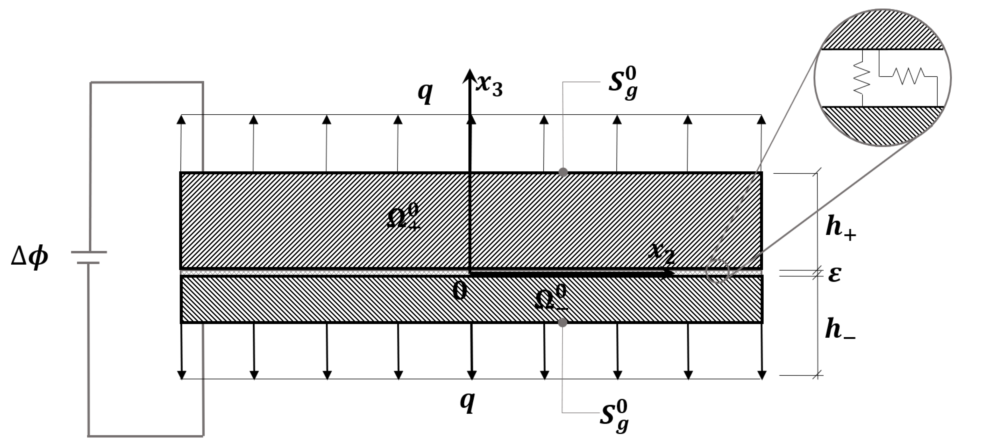
Let us consider an assembly composed of two piezoelectric adherent parallelepipeds, ${\mathrm{\Omega }}_{-}^0$ and ${\mathrm{\Omega }}_{+}^0$, with identical lateral dimensions but possible different heights, $h_{-}$ and $h_{+}$ respectively. The two adherents are joined by a very thin piezoelectric damaging adhesive, so the governing equations of the composite are assumed to be given by (57). The whole body is subjected to a soft loading device, i.e., a tensile load $\mathbf{q}=q\mathbf{n}$, with $q>0,$ acting on the top and bottom surfaces, whose union is denoted $S_g^0,$ as represented in Figure 2. The lateral boundaries of ${\mathrm{\Omega }}_{-}^0$ and ${\mathrm{\Omega }}_{+}^0$ are free from surface forces and the surface charge density w is negligible everywhere on the boundary.

The adherents are assumed to be made of orthotropic piezoelectric materials with poling axis ${\mathbf{i}}_3,$ whose constitutive tensors take, in Voigt’s notation, the following form:

$${\mathbf{C}}^{\pm }=\left[\begin{array}{cccccc}{c}_{11}^{\pm }& c_{12}^{\pm }& c_{13}^{\pm }& 0& 0& 0\\ c_{12}^{\pm }& c_{22}^{\pm }& c_{23}^{\pm }& 0& 0& 0\\ c_{13}^{\pm }& c_{23}^{\pm }& c_{33}^{\pm }& 0& 0& 0\\ 0& 0& 0& c_{44}^{\pm }& 0& 0\\ 0& 0& 0& 0& c_{55}^{\pm }& 0\\ 0& 0& 0& 0& 0& c_{66}^{\pm }\end{array}\right],$$

(61)

$${\mathbf{P}}^{\pm }=\left[\begin{array}{ccc}0& 0& p_{31}^{\pm }\\ 0& 0& p_{32}^{\pm }\\ 0& 0& p_{33}^{\pm }\\ 0& p_{24}^{\pm }& 0\\ p_{25}^{\pm }& 0& 0\\ 0& 0& 0\end{array}\right],$$

(62)

$${\mathbf{H}}^{\pm }=\left[\begin{array}{ccc}{h}_{11}^{\pm }& 0& 0\\ 0& h_{22}^{\pm }& 0\\ 0& 0& h_{33}^{\pm }\end{array}\right].$$

(63)

The adhesive is made of a transversely isotropic material with poling axis ${\mathbf{i}}_3.$ The matrices ${\widehat{\mathbf{C}}}^{\epsilon ,33}$ and ${\widehat{\mathbf{P}}}^{\epsilon ,33}$ appearing in the transmission conditions of the system of governing Equation (57) take the form

$${\widehat{\mathbf{C}}}^{\epsilon ,33}=\left[\begin{array}{ccc}{\widehat{c}}_{55}^{\epsilon }\left(\lambda \right)& 0& 0\\ 0& {\widehat{c}}_{55}^{\epsilon }\left(\lambda \right)& 0\\ 0& 0& {\widehat{c}}_{33}^{\epsilon }\left(\lambda \right)\end{array}\right],$$

(64)

$${\widehat{\mathbf{P}}}^{\epsilon ,33}=\left[\begin{array}{c}0\\ 0\\ {\widehat{p}}_{33}^{\epsilon }\left(\lambda \right)\end{array}\right],$$

(65)

respectively, and one has

$${\widehat{H}}^{\epsilon ,33}={\widehat{h}}_{33}^{\epsilon }\left(\lambda \right).$$

(66)

The dependence on the damage parameter $\lambda$ will be specified later.

The following choice:

$$\left\{\begin{array}{cc}{\mathbf{u}}_{\pm }^0=q\sum _{i=1}^3{C}_i^{\pm }{x}_i{\mathbf{i}}_i+u_3^{\pm }{\mathbf{i}}_3\hfill & \mathrm{in}{\mathrm{\Omega }}_{\pm }^0,\hfill \\ {\varphi }_{\pm }^0=-q{C}_4^{\pm }{x}_3+{\varphi }^{\pm }\hfill & \mathrm{in}{\mathrm{\Omega }}_{\pm }^0,\hfill \\ {\sigma }^0=q({\mathbf{i}}_3\otimes {\mathbf{i}}_3)\hfill & \mathrm{in}{\mathrm{\Omega }}_{+}^0\cup {\mathrm{\Omega }}_{-}^0,\hfill \\ {\mathbf{D}}^0=\mathbf{0}\hfill & \mathrm{in}{\mathrm{\Omega }}_{+}^0\cup {\mathrm{\Omega }}_{-}^0,\hfill \end{array}\right.$$

(67)

satisfies the first eight equations of (57). The expressions of the constants $C_K^{\pm },K=1,2,3,4$, are given in the Appendix A. The choice (67) corresponds to a piezoelectric state $({\mathbf{u}}^0,{\varphi }^0)$ homogeneous in the adherents and superimposed to jump discontinuities $\left[u_3^0\right]=(u_3^{+}-u_3^{-})$ and $\left[{\varphi }^0\right]=({\varphi }^{+}-{\varphi }^{-})$ concentrated at the adhesive interface $S.$

Substituting (64)–(67) into the ninth and tenth equations of the system (57), the following values for the jumps $\left[u_3^0\right]$ and $\left[{\varphi }^0\right]$ are obtained:

$$\begin{array}{ccc}\hfill {\displaystyle \frac{\left[u_3^0\right]}{\epsilon }}& =& {\displaystyle \frac{q{h}_{33}^{\epsilon }\left(\lambda \right)}{c_{33}^{\epsilon }\left(\lambda \right)h_{33}^{\epsilon }\left(\lambda \right)+{\left(p_{33}^{\epsilon }\left(\lambda \right)\right)}^2},}\hfill \end{array}$$

(68)

$$\begin{array}{ccc}\hfill {\displaystyle \frac{\left[{\varphi }^0\right]}{\epsilon }}& =& {\displaystyle \frac{q{p}_{33}^{\epsilon }\left(\lambda \right)}{c_{33}^{\epsilon }\left(\lambda \right)h_{33}^{\epsilon }\left(\lambda \right)+{\left(p_{33}^{\epsilon }\left(\lambda \right)\right)}^2}.}\hfill \end{array}$$

(69)

In view of (68) and (69), it is now possible to calculate the macroscopic strain of the composite along the thickness direction (i.e., ${\mathbf{i}}_3$)

$$\begin{array}{ccc}\hfill ϵ& :=& {\displaystyle \frac{u_3^0(x_1,x_2,h_{+})-u_3^0(x_1,x_2,-h_{-})}{h_{+}+h_{-}}}\hfill \\ & =& {\displaystyle q{\zeta }^{+}{C}_3^{+}+q{\zeta }^{-}{C}_3^{-}+q\zeta \frac{h_{33}^{\epsilon }\left(\lambda \right)}{c_{33}^{\epsilon }\left(\lambda \right)h_{33}^{\epsilon }\left(\lambda \right)+{\left(p_{33}^{\epsilon }\left(\lambda \right)\right)}^2},}\hfill \end{array}$$

(70)

with

$${\displaystyle {\zeta }^{\pm }:=\frac{h_{\pm }}{h_{+}+h_{-}},\zeta :=\frac{\epsilon }{h_{+}+h_{-}},}$$

(71)

the volume fractions of the three layers. The voltage per unit height between the top and bottom bases of the composite is

$$\begin{array}{ccc}\hfill {\displaystyle \frac{\mathrm{\Delta }\varphi }{h_{+}+h_{-}}}& :=& {\displaystyle \frac{{\varphi }^0(x_1,x_2,h_{+})-{\varphi }^0(x_1,x_2,-h_{-})}{h_{+}+h_{-}}}\hfill \\ & =& {\displaystyle q{\zeta }^{+}{C}_4^{+}+q{\zeta }^{-}{C}_4^{-}+q\zeta \frac{p_{33}^{\epsilon }\left(\lambda \right)}{c_{33}^{\epsilon }\left(\lambda \right)h_{33}^{\epsilon }\left(\lambda \right)+{\left(p_{33}^{\epsilon }\left(\lambda \right)\right)}^2}.}\hfill \end{array}$$

(72)

The inverse piezoelectric coefficient, defined by

$$\begin{array}{ccc}\hfill d& :=& {\displaystyle \frac{ϵ}{{\displaystyle \frac{\mathrm{\Delta }\varphi }{h_{+}+h_{-}}}},}\hfill \end{array}$$

(73)

can be computed from the expressions (70) and (72). Parameter d measures the ability of the structure to develop the inverse piezoelectric effect, converting electrical energy to mechanical energy.

The macroscopic quantities $ϵ,$$\mathrm{\Delta }\varphi /(h_{+}+h_{-})$ and d depend upon the damage parameter $\lambda$ and its evolution, described by the last equation of the system (57). Substituting (64)–(67) into the last equation of the system (57), the following differential equation in $\lambda$ is obtained:

$${\widehat{\eta }}^{\epsilon }\dot{\lambda }={\left({\displaystyle {\widehat{\omega }}^{\epsilon }-\frac{1}{2}{\widehat{c}}_{33,\lambda }^{\epsilon }\left(\lambda \right){\left({\displaystyle \frac{\left[u_3^0\right]}{\epsilon }}\right)}^2-\frac{1}{2}{\widehat{h}}_{33,\lambda }^{\epsilon }\left(\lambda \right){\left({\displaystyle \frac{\left[{\varphi }^0\right]}{\epsilon }}\right)}^2+{\widehat{p}}_{33,\lambda }^{\epsilon }\left(\lambda \right)\frac{\left[u_3^0\right]}{\epsilon }\frac{\left[{\varphi }^0\right]}{\epsilon }}\right)}_{+},$$

(74)

that, in view of (68) and (), becomes

$${\widehat{\eta }}^{\epsilon }\dot{\lambda }={\left({\displaystyle {\widehat{\omega }}^{\epsilon }-q^2\frac{{\left({\widehat{h}}_{33}^{\epsilon }\left(\lambda \right)\right)}^2{\widehat{h}}_{33,\lambda }^{\epsilon }\left(\lambda \right)+{\widehat{c}}_{33,\lambda }^{\epsilon }\left(\lambda \right){\left({\widehat{p}}_{33}^{\epsilon }\left(\lambda \right)\right)}^2-2{\widehat{h}}_{33}^{\epsilon }\left(\lambda \right){\widehat{p}}_{33}\left(\lambda \right){\widehat{p}}_{33,\lambda }^{\epsilon }\left(\lambda \right)}{{\widehat{c}}_{33}^{\epsilon }\left(\lambda \right){\widehat{h}}_{33}^{\epsilon }\left(\lambda \right)+{\left({\widehat{p}}_{33}^{\epsilon }\left(\lambda \right)\right)}^2}}\right)}_{+},$$

(75)

to be completed with an initial condition for $\lambda :$

$$\lambda \left(0\right)={\lambda }_0.$$

(76)

As for the dependence of the material parameters of the adhesive on $\lambda ,$ we follow the Kachanov–Sevostianov homogenization scheme [45,46,47,48], where the parameters of the adhesive, ${\widehat{c}}_{33}^{\epsilon },{\widehat{p}}_{33}^{\epsilon },$ and ${\widehat{h}}_{33}^{\epsilon }$ depend on $\lambda$ as follows:

$$\begin{array}{ccc}\hfill {\widehat{c}}_{33}^{\epsilon ,KS}& =& {\displaystyle \frac{{\widehat{c}}_{33}^0}{1+2\pi \lambda }},\hfill \\ \hfill {\widehat{p}}_{33}^{\epsilon ,KS}& =& {\displaystyle \frac{{\widehat{p}}_{33}^0}{1+2\pi \lambda }},\hfill \\ \hfill {\widehat{h}}_{33}^{\epsilon ,KS}& =& {\displaystyle \frac{{\widehat{h}}_{33}^0}{1+2\pi \lambda }},\hfill \end{array}$$

(77)

with ${\widehat{c}}_{33}^0,{\widehat{p}}_{33}^0,$ and ${\widehat{h}}_{33}^0$ corresponding to the values of the undamaged material parameters.

Substituting the relations (77) into the evolution Equation (75), we obtain the simple linear differential equation

$$\eta \dot{\lambda }={\left(\omega +c{q}^2\right)}_{+}$$

(78)

with

$${\displaystyle c=\frac{\pi {\widehat{h}}_{33}^0({\widehat{c}}_{33}^0{\widehat{h}}_{33}^0-{\left({\widehat{p}}_{33}^0\right)}^2)}{{({\widehat{c}}_{33}^0{\widehat{h}}_{33}^0+{\left({\widehat{p}}_{33}^0\right)}^2)}^2}.}$$

(79)

Now assume that the load q is time dependent, $q=q\left(t\right)$ with $t\ge 0,$ and assume that ${\lambda }_0=0.$ For times t such that

$$q^2\left(t\right)=-\frac{\omega }{c}$$

(80)

damage initiates. Let $t_0$ be the first solution of such equation. For $0<t<t_0,$ no damage occurs, i.e., $\lambda \left(t\right)={\lambda }_0=0$ and the mechanical and electric responses of the composite are classical and linear. For $t\ge t_0,$ damage initiates and evolves according to the following first integral of (78):

$$\lambda \left(t\right)=\frac{\omega }{\eta }t+\frac{\omega }{c}{\int }_0^t{q}^2\left(s\right)ds.$$

(81)

The macroscopic response of the composite described by relations (70) and (72) is non linear, due to Equation (81) describing non linear damage evolution. In the next subsection, we calculate numerically the macroscopic response of the composite for a typical configuration under cyclic traction.

Simulation of the Macroscopic Response for a PZT-4/PVDF Composite under Cyclic Traction

For the composite sketched in Figure 2, the adherents are assumed to be constituted by PZT-4 and the damaging thin layer of PVDF, whose material parameters are listed in

Table 1. Constitutive coefficients of the adherents [55].

	${\mathit{c}}_{11}^{\pm }$	${\mathit{c}}_{22}^{\pm }$	${\mathit{c}}_{33}^{\pm }$	${\mathit{c}}_{12}^{\pm }$	${\mathit{c}}_{13}^{\pm }$	${\mathit{c}}_{23}^{\pm }$	${\mathit{p}}_{31}^{\pm }$	${\mathit{p}}_{32}^{\pm }$	${\mathit{p}}_{33}^{\pm }$	${\mathit{h}}_{33}^{\pm }$
	GPa	GPa	GPa	GPa	GPa	GPa	cm${}^{-2}$	cm${}^{-2}$	cm${}^{-2}$	nFm${}^{-1}$
PZT-4	139	139	115	77.8	74.3	74.3	−5.2	−5.2	15.1	11.51

and

Table 2. Constitutive coefficients of the thin adhesive [55]. The values in the table refer to the material in undamaged conditions.

	${\widehat{\mathit{c}}}_{33}^0$	${\widehat{\mathit{p}}}_{33}^0$	${\widehat{\mathit{h}}}_{33}^0$
	GPa	cm${}^{-2}$	nFm${}^{-1}$
PVDF	10.64	−0.276	0.106

.

The load $q,$ is assumed to be piece-wise linear in time, thus simulating cyclic loading and unloading ramps. Noting $\dot{q}$ ($-\dot{q}$), $t_0$ and $t_f$ the loading (unloading) rate, the time of damage initiation and the half period, respectively, from Equation (80) and the linearity of $q\left(t\right),$ it follows that the damage initiation time takes the form

$${\displaystyle t_0=\frac{\sqrt{-\omega }}{\dot{q}\sqrt{c}}.}$$

(82)

We assume that $t_f>t_0,$ so damage occurs before the ending of each loading ramp.

In Figure 3, Figure 4, Figure 5, Figure 6 and Figure 7, the results of simulations are shown, obtained by implementing equations (61) into (81) for a single loading–unloading cycle and for three loading–unloading cycles. To perform the calculations, the symbolic software Mathematica was used [56]. The numerical values of the loading and material parameters are listed in Table 1, Table 2 and

Table 3. Loading and damage material parameters used for the simulated macroscopic responses plotted in Figure 2, Figure 3 and Figure 4.

$\dot{\mathit{q}}$	${\mathit{\lambda }}_0$	$\mathit{\eta }$	$\mathit{\omega }$
Pa/s	-	N s/m	N/m
		0.1	−0.1
${10}^4$	0	1.0	−1.0
		10.0

. In the simulations, different values for the parameters $\eta$ and $\omega$ have been considered, to highlight the different effect of these two parameters on the composite behaviour. Be noted that the damage initiation time (82) depends upon $\omega ,$ thus varying the latter corresponds to consider different loading histories.

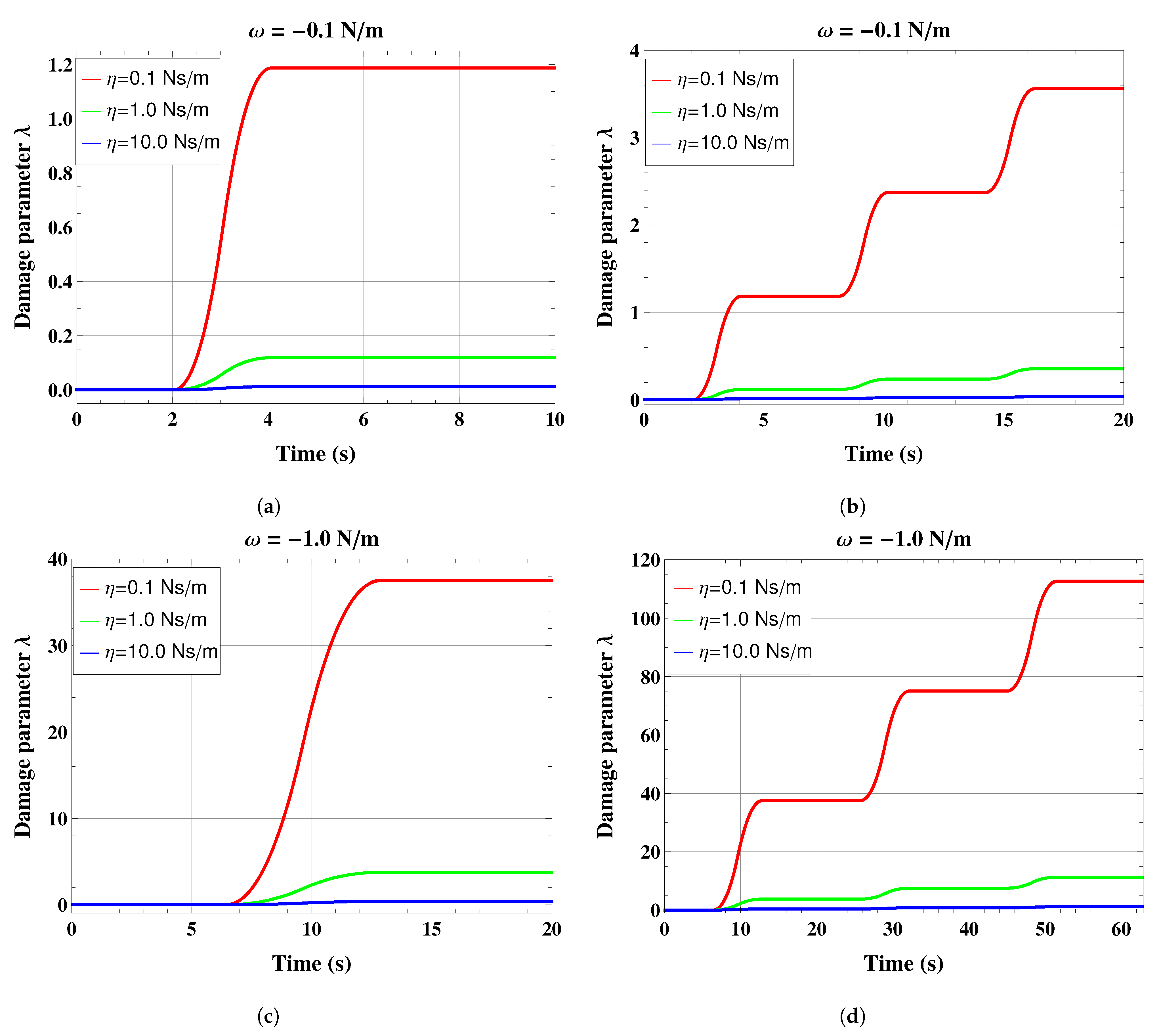
Figure 3 shows the time evolution of the damage parameter $\lambda$ in a single loading–unloading cycle (SC) and in three loading–unloading cycles (MC). The case of pure elastic behavior in absence of damage (E) corresponds to a fixed $\lambda =0$ for all times. Damage nucleates at $t_0=2.03$ s for $\omega =-0.1$ N/m and at $t_0=6.43$ s for $\omega =-1.0$ N/m, as it can be calculated using Equation (82) with the values provided in Table 3. Then, damage increases until the end of loading ramps, following which it remains constant until the end of the unloading phases. This behavior gives a wavy appearance to the curves for multiple cycles. Damage is larger for smaller values of the parameter $\eta ,$ i.e., high viscosity delays damage evolution, as also found in [50].

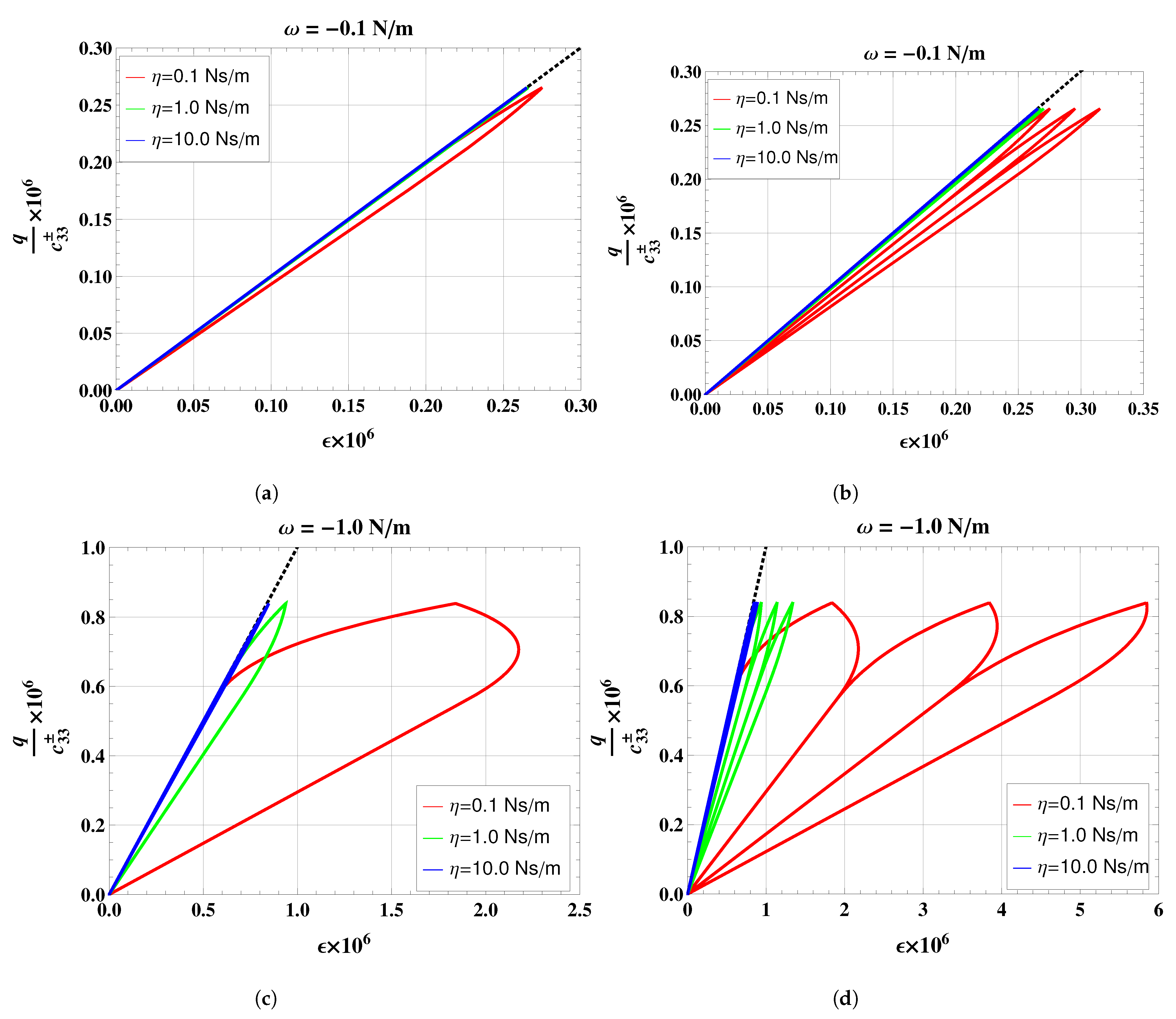
The normalized stress versus strain response and normalized stress versus normalized potential per unit height response are shown in Figure 4 and Figure 5, respectively. Figure 6 shows the normalized strain versus normalized potential per unit height response. The three figures highlight the occurrence of an elastic-damaging material behavior with hysteresis. Higher hysteresis is associated with smaller values of $\eta$ and larger values of $\omega ,$ and the hysteresis is wider for the normalized stress-strain and stress-potential responses. In the MC case, during the unloading phases, the slope of all response functions decrease with the number of cycles. This corresponds to elastic damage accumulation in the thin layer during the loading history.

Figure 7 shows the evolution of the normalized inverse piezoelectric coefficient (73) with time. The plots show that damage accumulation decreases the coefficient and the effect is more pronounced for smaller values of $\eta$ and larger values of $\omega .$

In the literature, damage progression under cyclic loading is usually evaluated via stiffness degradation. Let $E_N$ be taken to denote the ratio between the maximum applied load at cycle N and the corresponding strain. Stiffness degradation can be defined as $E_N/E_1,$ with $E_1$ the ratio between the maximum applied load at the first cycle and the corresponding strain. Stiffness degradation versus the number of cycle is shown in the plot of the left-hand side of Figure 8 for the first 30 cycles and material parameters $\omega =-0.1$ N/m and $\eta =0.1$ Ns/m. The plot on the right-hand side of Figure 8 shows the degradation of the inverse piezoelectric coefficient versus the cycle number for the same values of the material parameters $\omega$ and $\eta .$ The two plots indicate that the first loading cycles are characterized by a rapid degradation of stiffness and inverse piezoelectric effect, followed by a more gradual reduction. This behavior is qualitatively consistent with experimental observations of stiffness degradation obtained on cyclic compression of piezoelectric PVDF foams (p. 191, [57]). This provides a validation of the approach proposed in the present paper and shows its usefulness.

5. Conclusions

This work proposes an original imperfect interface model for damage description in thin-film piezoelectric materials. The model is set in the framework of damage continuum mechanics and it is based on Kachanov and Sevostianov’s results of homogenization of micro-cracked media and on asymptotic analysis for the derivation of the interface law. The resulting interface model views the film as a piezoelectric material surface undergoing micro-cracking and subsequent damage evolution and accumulation.

To illustrate the application of the interface model, an academic example has been presented based on two piezoelectric PZT-4 adherent layers joined by a damaging thin PVDF film modeled as a damaging imperfect interface. The stack is subjected to cyclic loading and unloading ramps and damage evolution is calculated. In the absence of damage the macroscopic response of the stack would be linear. However, when damage is accounted for via the interface law, the numerical results show that the macroscopic response in terms of stress, strain and potential become non-linear and hysteresis occurs. The numerical analysis shows that the elastic and piezoelectric behavior of the stack tends to deteriorate as the number of cycles increases.

Interestingly, the interface model presents two free parameters, $\eta$ and $\omega ,$ representing respectively a damage viscosity and a damage energy threshold and both are related to the damage evolution law. The numerical analysis, performed for different values of $\eta$ and $\omega ,$ has highlighted the specific effect of the two parameters: large values of $\omega$ delay damage initiation, while large values of the viscosity parameter $\eta$ delay damage evolution.

As an additional result of the numerical analysis, the evolution of the normalized inverse piezoelectric coefficient of the layered composite in single loading–unloading cycles and in multiple loading–unloading cycles has been evaluated. The normalized inverse piezoelectric is determinant for the actuation, so the possibility of evaluating how damage affects this coefficient suggests that the proposed model could be a viable strategy for modeling fatigue of piezoelectric thin film materials.

Introducing the concept of stiffness degradation, our numerical results indicate that the simulated behavior of the PZT-4/PVDF stack is in qualitative agreement with experimental observations [57]. This important aspect provides a validation of the proposed model.

Finally, since piezoelectric thin films are very suitable for a variety of applications in MEMS, such as high energy density harvesters and high sensitivity sensors [5], the content presented in the present paper is expected to be useful for evaluating damage evolution and correspondingly design safe operational cyclic loading in such applications. Moreover, taking into account that wet and dry bone composite structures show piezoelectric effect (see the pioneering work by E. Fukada and I. Yasuda [58]), the present work can be considered relevant to shed light on the complex problem of damage-bone remodelling subjected to electromechanical stimulation, as in e.g., [59,60].

References

- Muralt, P.; Polcawich, R.; Trolier-McKinstry, S. Piezoelectric Thin Films for Sensors, Actuators, and Energy Harvesting. MRS Bull. 2009, 34, 658–664. [Google Scholar] [CrossRef] [Green Version]
- Rjafallah, A.; Hajjaji, A.; Belhora, F.; Guyomar, D.; Seveyrat, L.; El Otmani, R.; Boughaleb, Y. Mechanical energy harvesting using polyurethane/lead zirconate titanate composites. J. Compos. Mater. 2018, 52, 1171–1182. [Google Scholar] [CrossRef]
- Safaei, M.; Sodano, H.A.; Anton, S.R. A review of energy harvesting using piezoelectric materials: State-of-the-art a decade later (2008–2018). Smart Mater Struct. 2019, 28, 113001. [Google Scholar] [CrossRef]
- Salazar, R.; Serrano, M.; Abdelkefi, A. Fatigue in piezoelectric ceramic vibrational energy harvesting: A review. Appl. Energy 2020, 270, 115161. [Google Scholar] [CrossRef]
- Kanno, I. Piezoelectric MEMS: Ferroelectric thin films for MEMS applications. Jpn. J. Appl. Phys. 2018, 57, 040101. [Google Scholar] [CrossRef] [Green Version]
- Gao, W.; Zhu, Y.; Wang, Y.; Yuan, G.; Liu, J.-M. A review of flexible perovskite oxide ferroelectric films and their application. J. Mater. 2020, 6, 1–16. [Google Scholar] [CrossRef]
- Caillerie, D. The effect of a thin inclusion of high rigidity in an elastic body. Math. Methods Appl. Sci. 1980, 2, 251–270. [Google Scholar] [CrossRef]
- Hashin, Z. Thin interphase/imperfect interface in elasticity with application to coated fiber composites. J. Mech. Phys. Solids 2002, 50, 2509–2537. [Google Scholar] [CrossRef]
- Geymonat, G.; Hendili, S.; Krasucki, F.; Serpilli, M.; Vidrascu, M. Asymptotic expansions and domain decomposition. Lect. Notes Comput. Sci. Eng. 2014, 98, 749–757. [Google Scholar]
- Klarbring, A. Derivation of the adhesively bonded joints by the asymptotic expansion method. Int. J. Eng. Sci. 1991, 29, 493–512. [Google Scholar] [CrossRef]
- Benveniste, Y. The effective conductivity of composites with imperfect thermal contact at constituent interfaces. Int. J. Eng. Sci. 1986, 24, 1537–1552. [Google Scholar] [CrossRef]
- Benveniste, Y. Effective thermal-conductivity of composites with a thermal contact resistance between the constituents-nondilute case. J. Appl. Phys. 1987, 61, 2840–2843. [Google Scholar] [CrossRef]
- Javili, A.; Kaessmair, S.; Steinmann, P. General imperfect interfaces. Comput. Methods Appl. Mech. Eng. 2014, 275, 76–97. [Google Scholar] [CrossRef]
- Javili, A. Variational formulation of generalized interfaces for finite deformation elasticity. Math. Mech. Solids 2018, 23, 1303–1322. [Google Scholar] [CrossRef]
- Serpilli, M.; Dumont, S.; Rizzoni, R.; Lebon, F. Interface models in coupled thermoelasticity. Technologies 2021, 9, 17. [Google Scholar] [CrossRef]
- Lebon, F.; Rizzoni, R. Asymptotic behavior of a hard thin linear interphase: An energy approach. Int. J. Solid Struct. 2011, 48, 441–449. [Google Scholar] [CrossRef] [Green Version]
- Rizzoni, R.; Dumont, S.; Lebon, F.; Sacco, E. Higher order model for soft and hard elastic interfaces. Int. J. Solid Struct. 2014, 51, 4137–4148. [Google Scholar] [CrossRef]
- Dumont, S.; Rizzoni, R.; Lebon, F.; Sacco, E. Soft and hard interface models for bonded elements. Compos. B Eng. 2018, 153, 480–490. [Google Scholar] [CrossRef] [Green Version]
- Serpilli, M.; Lenci, S. Asymptotic modelling of the linear dynamics of laminated beams. Int. J. Solids Struct 2012, 49, 1147–1157. [Google Scholar] [CrossRef] [Green Version]
- Furtsev, A.; Rudoy, E. Variational approach to modeling soft and stiff interfaces in the Kirchhoff-Love theory of plates. Int. J. Solid Struct. 2020, 202, 562–574. [Google Scholar] [CrossRef]
- Serpilli, M.; Lenci, S. An overview of different asymptotic models for anisotropic three-layer plates with soft adhesive. Int. J. Solids Struct 2016, 81, 130–140. [Google Scholar] [CrossRef]
- Rizzoni, R.; Dumont, S.; Lebon, F. On Saint Venant-Kirchhoff imperfect interfaces. Int. J. Nonlin. Mech. 2017, 89, 101–115. [Google Scholar] [CrossRef] [Green Version]
- Lebon, F.; Rizzoni, R. On the emergence of adhesion in asymptotic analysis of piecewise linear anisotropic elastic bonded joints. Eur. J. Mech. -A/Solid 2022, 93, 104512. [Google Scholar] [CrossRef]
- Serpilli, M. On modeling interfaces in linear micropolar composites. Math. Mech. Solids 2018, 23, 667–685. [Google Scholar] [CrossRef]
- Serpilli, M. Classical and higher order interface conditions in poroelasticity. Ann. Solid Struct. Mech. 2019, 11, 1–10. [Google Scholar] [CrossRef]
- Serpilli, M. Mathematical modeling of weak and strong piezoelectric interfaces. J. Elast. 2015, 121, 235–254. [Google Scholar] [CrossRef]
- Serpilli, M.; Rizzoni, R.; Lebon, F.; Dumont, S. Higher order interface conditions for piezoelectric spherical hollow composites: Asymptotic approach and transfer matrix homogenization method. Compos. Struct. 2022, 279, 114760. [Google Scholar] [CrossRef]
- Serpilli, M. Asymptotic interface models in magneto-electro-thermo-elastic composites. Meccanica 2017, 52, 1407–1424. [Google Scholar] [CrossRef]
- Serpilli, M.; Rizzoni, R.; Rodríguez-Ramos, R.; Lebon, F.; Dumont, S. A novel form of imperfect contact laws in flexoelectricity. Compos. Struct. 2022, 300, 116059. [Google Scholar] [CrossRef]
- Serpilli, M.; Rizzoni, R.; Lebon, F.; Dumont, S. An asymptotic derivation of a general imperfect interface law for linear multiphysics composites. Int. J. Solids Struct. 2019, 180–181, 97–107. [Google Scholar] [CrossRef] [Green Version]
- Dumont, S.; Serpilli, M.; Rizzoni, R.; Lebon, F. Numerical validation of multiphysic imperfect interfaces models. Front. Mater. 2020, 158, 1–13. [Google Scholar] [CrossRef]
- Lemaitre, J.; Chaboche, J.-L. Mechanics of Solid Materials; Cambridge University Press: Cambridge, UK, 1990. [Google Scholar]
- Lemaitre, J. A Course on Damage Mechanics; Springer: Berlin, Germany, 1992. [Google Scholar]
- Park, T.; Ahmed, B.; Voyiadjis, G.Z. A review of continuum damage and plasticity in concrete: Part I-Theoretical framework. Int. J. Damage Mech. 2022, 31, 901–954. [Google Scholar] [CrossRef]
- Kachanov, M.L. Time of the rupture process under creep conditions. Izv. Akad. Nauk. (S.S.R.) Otd. Tech. Nauk 1958, 8, 26–31. [Google Scholar]
- Rabotnov, Y.N. On the Mechanism of Delayed Fracture; Izd. Akad. Nauk SSSR: Moscow, Russia, 1959; pp. 5–7. [Google Scholar]
- Voyiadjis, G.Z.; Kattan, P.I. Fundamental aspects for characterization in continuum damage mechanics. Int. J. Damage Mech. 2019, 28, 200–218. [Google Scholar] [CrossRef]
- Li, X.; Gao, W.; Liu, W. A mesh objective continuum damage model for quasi-brittle crack modelling and finite element implementation. Int. J. Damage Mech. 2019, 28, 1299–1322. [Google Scholar] [CrossRef]
- Ottosen, N.S.; Stenströ, R.; Ristinmaa, M. Continuum approach to high-cycle fatigue modeling. Int. J. Fatigue 2008, 30, 996–1006. [Google Scholar] [CrossRef]
- Lindström, S.; Thore, C.; Suresh, S.; Klarbring, A. Continuous-time, high-cycle fatigue model: Validity range and computational acceleration for cyclic stress. Int. J. Fatigue 2020, 136, 105582. [Google Scholar] [CrossRef]
- Suresh, S.; Lindström, S.B.; Thore, C.J.; Klarbring, A. Acceleration of continuous-time, high-cycle fatigue constrained problems in topology optimization. Eur. J. Mech. A Solids 2022, 96, 104723. [Google Scholar] [CrossRef]
- Mizuno, M. Constitutive Equation of Piezoelectric Ceramics Taking into Account Damage Development. Key Eng. Mater. 2003, 233–236, 89–94. [Google Scholar]
- Mizuno, M.; Okayasu, M.; Odagiri, N. Damage Evaluation of Piezoelectric Ceramics from the Variation of the Elastic Coefficient under Static Compressive Stress. Int. J. Damage Mech. 2010, 19, 375–390. [Google Scholar] [CrossRef]
- Yang, X.H.; Chen, C.Y.; Hu, Y.T. A Static Damage Constitutive Model for Piezoelectric Materials. In Mechanics of Electromagnetic Solids; Advances in Mechanics and Mathematics; Yang, J.S., Maugin, G.A., Eds.; Springer: Boston, MA, USA, 2003; Volume 3. [Google Scholar]
- Kachanov, M.; Sevostianov, I. On quantitative characterization of microstructures and effective properties. Int. J. Solid Struct. 2005, 42, 309–336. [Google Scholar] [CrossRef]
- Kachanov, M.; Sevostianov, I. Micromechanics of Materials, with Applications; Springer: Cham, Switzerland, 2018; Volume 249. [Google Scholar]
- Sevostianov, I.; Kachanov, M. On some controversial issues in effective field approaches to the problem of the overall elastic properties. Mech. Mat. 2014, 69, 93–105. [Google Scholar] [CrossRef]
- Kachanov, M. Elastic solids with many cracks and related problems. Adv. Appl. Mech. 1994, 30, 259–445. [Google Scholar]
- Bonetti, E.; Bonfanti, G.; Lebon, F.; Rizzoni, R. A model of imperfect interface with damage. Meccanica 2017, 52, 1911–1922. [Google Scholar] [CrossRef]
- Raffa, M.L.; Lebon, F.; Rizzoni, R. A micromechanical model of a hard interface with micro-cracking damage. Int. J. Mech. Sci. 2022, 216, 106974. [Google Scholar] [CrossRef]
- Frémond, M. Non-Smooth Thermo-Mechanics, 3rd ed.; Springer: Berlin, Germany, 2001. [Google Scholar]
- Fouchal, F.; Lebon, F.; Titeux, I. Contribution to the modelling of interfaces in masonry construction. Const. Build. Mat. 2009, 23, 2428–2441. [Google Scholar] [CrossRef] [Green Version]
- Frémond, M.; Nedjar, B. Damage, gradient of damage and priciple of virtual power. Int. J. Solid Struct. 1996, 33, 1083–1103. [Google Scholar] [CrossRef]
- Ciarlet, P.G. Mathematical Elasticity. Volume II: Theory of Plates. In Series Studies in Mathematics and its Applications; Elsevier: Amsterdam, The Netherlands, 1997. [Google Scholar]
- Fernades, A.; Pouget, J. An accurate modelling of piezoelectric multi-layer plates. Eur. J. Mech. A Solids 2002, 21, 629–651. [Google Scholar] [CrossRef] [Green Version]
- Wolfram Research, Inc. Mathematica, Version 13.0.0; Wolfram Research, Inc.: Champaign, IL, USA, 2021.
- Frioui, N.; Bezazi, A.; Remillat, C.; Scarpa, F.; Gomez, J.P. Viscoelastic and compression fatigue properties of closed cell PVDF foam. Mech. Mat. 2010, 42, 189–195. [Google Scholar] [CrossRef]
- Fukada, E.; Yasuda, I. On the piezoelectric effect of bone. J. Phys. Soc. (Jpn.) 1957, 12, 1158–1162. [Google Scholar] [CrossRef]
- Ramtani, S.; Zidi, M. A theoretical model of the effect of continuum damage on a bone adaptation model. J. Biomech. 2001, 34, 471–479. [Google Scholar] [CrossRef] [PubMed]
- Ramtani, S. Electro-mechanics of bone remodelling. Int. J. Eng. Sci. 2008, 46, 1173–1182. [Google Scholar] [CrossRef]
Figure 1.
Geometry of the bonded assembly composed of two adherent bodies and an adhesive thin layer: reference configuration (a), rescaled configuration (b) and limit configuration (c).
Figure 2.
A piezoelectric three-layered composite body subject to soft loading. The intermediate thin layer is made of a damaging material.
Figure 3.
Damage evolution in a single loading–unloading cycle (a,c) and in multiple loading–unloading cycles (b,d) of the layered composite depicted in Figure 2. The different plots show the effect of varying and in in the damage evolution Equation (75).
Figure 4.
Normalized stress versus strain response in a single loading–unloading cycle (a,c) and in multiple loading–unloading cycles (b,d) of the layered composite depicted in Figure 2. The different plots show the effect of varying and in in the damage evolution Equation (75). For comparison, normalized stress versus strain response in absence of damage (purely elastic case) is represented with a dotted line.
Figure 5.
Normalized stress versus normalized potential per unit height in a single loading–unloading cycle (a,c) and in multiple loading–unloading cycles (b,d) of the layered composite depicted in Figure 2. The different plots show the effect of varying and in in the damage evolution Equation (75). For comparison, normalized stress versus normalized potential per unit height in the purely elastic case is represented with a dotted line.
Figure 6.
Strain versus normalized potential per unit height in a single loading–unloading cycle (a,c) and in multiple loading–unloading cycles (b,d) of the layered composite depicted in Figure 2. The different plots show the effect of varying and in in the damage evolution Equation (75). For comparison, strain versus normalized potential per unit height in the purely elastic case is represented with a dotted line.
Figure 7.
Evolution of the normalized inverse piezoelectric coefficient in a single loading–unloading cycle (a,c) and in multiple loading–unloading cycles (b,d) of the layered composite depicted in Figure 2. The different plots show the effect of varying and in in the damage evolution Equation (75). For comparison, the normalized inverse piezoelectric coefficient in the purely elastic case is represented with a dotted line.
Figure 8.
Stiffness degradation (a) and inverse piezoelectric coefficient degradation (b) versus number of cycle for 30 loading cycles of the layered composite in Figure 2 for material parameters N/m and Ns/m.