
Micromechanical Modeling of Anisotropy and Strain Rate Dependence of Short-Fiber-Reinforced Thermoplastics

Department of Mechanical Engineering, Eindhoven University of Technology, P.O. Box 513, 5600 MB Eindhoven, The Netherlands
*
Author to whom correspondence should be addressed.
Fibers 2021, 9(7), 44; https://0-doi-org.brum.beds.ac.uk/10.3390/fib9070044
Submission received: 20 April 2021
/
Revised: 11 June 2021
/
Accepted: 28 June 2021
/
Published: 2 July 2021
(This article belongs to the Special Issue Simulation of Short-Fiber-Reinforced Polymers)
Abstract
:The anisotropy and strain rate dependence of the mechanical response of short-fiber-reinforced thermoplastics was studied using a straightforward micromechanical finite element analysis of representative volume elements (RVEs). RVEs are created based on the fiber orientation tensor, which quantifies the processing-induced fiber orientation distribution. The matrix is described by a strain rate-dependent constitutive model (the Eindhoven glassy polymer (EGP) model), which accurately captures the intrinsic response of amorphous polymers. The micromechanical results indicate that the influence of strain rate and that of the loading direction on the yield stress are multiplicatively decouplable, which confirms previous experimental observations. Moreover, it is demonstrated that the yield stress, to a good approximation, can be directly linked to the fiber orientation in the direction of loading. This leads to a new relation that uniquely links the rate dependence of the yield stress to the fiber orientation in loading direction.
1. Introduction
Due to their high specific strength, short-fiber-reinforced thermoplastics are currently used in a multitude of load-bearing applications where structural integrity and long-term reliability are key requirements, such as components used in automotive or aeronautic applications [1]. Hence, the ability to accurately predict the mechanical performance of such systems is of the utmost importance. Unfortunately, however, the accurate prediction of the performance of short-fiber-reinforced thermoplastic components still faces significant challenges.
One of these challenges is related to the fact that the yield strength of short-fiber-reinforced thermoplastics is generally strongly anisotropic due to processing-induced fiber orientation. During injection molding, the fibers are oriented during the flow of the molten fluid into the mold [2,3]. Due to spatial variation of the flow conditions throughout the mold, the material will display a marked variation in its anisotropic response on different positions of the molded product [4]. This intrinsic coupling between flow conditions and resulting mechanical properties makes the prediction of the mechanical performance of the molded part challenging. An additional complexity is that experimental observations clearly give evidence for a significant strain rate dependence of the yield strength on fiber-reinforced polymer composites [5,6,7,8]. Since the reinforcing fibers generally remain elastic until fracture [9], this dependence on strain rate is intrinsically related to the strain rate dependence of the mechanical response of the thermoplastic matrix, which is directly related to the influence of applied stress on chain mobility [10,11].
To adequately predict the strength of products based on fiber-reinforced thermoplastics, both the processing-induced fiber orientation as well as the strain rate dependence of the matrix must be considered. The difficulty in finding the optimal shape of a load-bearing component lies in the fact that changes in shape (even small ones) directly influence local flow conditions that subsequently alter the resulting fiber orientation distribution and the related anisotropic, time-dependent response. The inability to accurately predict the local anisotropic, rate-dependent mechanical properties directly from the fiber orientation distribution is the main cause that reliability of such products can only be warranted after full-scale testing—a time-consuming and costly procedure which hampers optimization.
Results from a recent study in our group, however, have opened a new, promising possibility to directly link fiber orientation to the anisotropic time-dependent response [12,13]. In an extensive experimental effort, it was demonstrated that the rate-dependent, anisotropic (yield) strength of short and long fiber-reinforced thermoplastics generally displays a multiplicative decoupling of the effects of strain rate and loading angle [12,13]. Additionally, it was shown that, at a fixed strain rate, the yield strength appears to be uniquely coupled to the average fiber orientation in the direction of testing [14]. This observation, in combination with the decomposition of the influence of strain rate and that of fiber orientation, could lead to a novel, fast method to accurately predict the anisotropic rate-dependent mechanical response for an arbitrary fiber orientation distribution.
The objective of the current manuscript was to further explore the experimentally observed decoupling of the orientation and strain rate dependence by using a micromechanical approach. Micromechanical modeling, based on the spatial fiber orientation distribution and the microscopic matrix behavior, is a method to intrinsically resolve the yield mechanism of composite materials. Compared to mean-field composite stiffness models, such as the Mori–Tanaka model [15,16] and pseudo-grain decomposition followed by two-step homogenization [17,18,19,20] of composite structures, full field models, such as that based on the finite element approach, are able to evaluate micro-level stress and the effects of interaction between adjacent inclusions on the overall properties. Micromechanical finite element analyses of representative volume elements of short-fiber-reinforced composites [21,22,23] showed good agreement between experimental and simulation results under some conditions, but the strain rate-dependent behavior of the composite was not taken into consideration.
A proper rate-dependent constitutive model for polymers is essential to predict the yield strength of the short-fiber-reinforced thermoplastics. A few researchers used a strain rate-dependent constitutive model and extended its utilization for polymer-based composites [24,25]. However, the constitutive model was developed based on the viscoplastic deformation of metals, and lacks the deformation kinetics of the polymers. A landmark in glassy polymer modeling was the pioneering work from Haward and Thackray [26], who proposed a model that considers the contributions of inter-molecular interactions and the molecular network to the mechanical properties. For a glassy polymer, the inter-molecular interactions, as a visco-elastic contribution, determine the moderate strain behavior including yield and strain softening. The molecular network, as a rubber-elastic contribution, governs the strain hardening behavior at large strains. Based on this pioneering work, further major developments were made by Boyce et al. (BPA model) [27,28,29], Buckley et al. (OGR model) [30,31] and our group in Eindhoven (EGP model) [32,33].
In this article, a fine-scale micromechanical finite element model was developed based on the rate-dependent Eindhoven glassy polymer (EGP) model for the thermoplastic matrix of short-fiber-reinforced composites and the processing-induced orientation of elastic fibers. This micromechanical model was used to investigate the anisotropic yield strength at the different strain rates and fiber orientation distributions. The experimentally observed multiplicative decoupling was proven in this study. Furthermore, a unique structure–property relation between the fiber orientation distribution and the anisotropic mechanical properties was found.
2. Micromechanical Modeling Approach
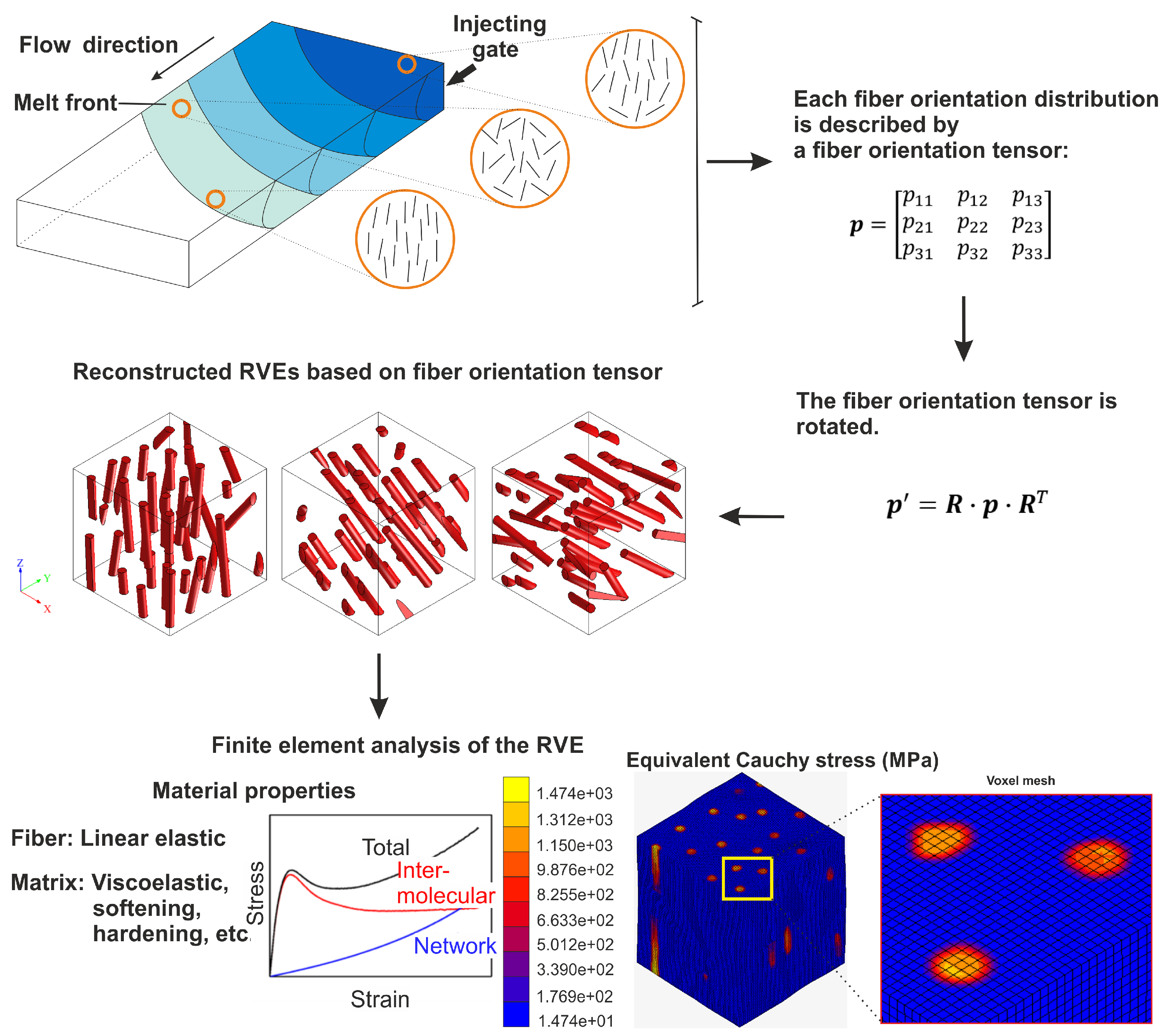
In this section, details of the micromechanical model for evaluating the anisotropic and rate-dependent behavior of short-fiber-reinforced thermoplastics are discussed. An E-glass short-fiber-reinforced polycarbonate material was considered. The anisotropic behavior was captured through finite element analyses (FEA) of representative volume elements (RVEs) at different loading angles. The rate-dependent behavior of the thermoplastic matrix was described with the Eindhoven glassy polymer (EGP) model. The fibers are modeled as isotropic elastic with a Young’s modulus of GPa and a Poisson’s ratio of . Fibers and matrix are assumed to be perfectly bonded. A schematic work flow of the micromechanical model is shown in Figure 1.
2.1. Representative Volume Elements
To quantify the fiber orientation distribution, the fiber orientation tensor [34] was introduced. The second order fiber orientation tensor is defined as the average of the dyadic product of orientation vectors for a number of m fibers [34]:
with the orientation vector of an individual fiber and where the trace of the fiber orientation tensor is equal to 1.
For investigating the anisotropic behavior of a microstructure, the fiber orientation tensor is rotated by different angles relative to the global coordinate system. The rotated fiber orientation tensor is given by
where is a rotation tensor. To conduct the finite element simulations of the E-glass short-fiber-reinforced polycarbonate, representative volume elements (RVEs) corresponding to different rotation angles which are generated using software package Digimat-FE 2018.1 [35], ensuring a geometric periodicity of the RVEs. This means that if a fiber passes one boundary, the remaining part of that fiber continues at the opposite side of the RVE. Consequently, if these RVEs are periodically stacked, a geometrically continuous structure is obtained. Due to computational limitations, an RVE with a low weight fraction and aspect ratio was considered in this paper. A total of 18 fibers with a weight fraction of (volume fraction ), diameter of mm and aspect ratio of 12 were distributed according to the fiber orientation tensor . Based on this geometric information, the RVE size was determined at . Consistent results were obtained for the RVE size of and prove the RVE size to be sufficiently large enough. The fibers were assumed to be cylindrical without intersection or contact. In addition, the fibers were separated as far as possible to avoid clustering effects through tuning the nearest neighboring distance. The representative volume elements are finally meshed with linear hexahedral solid elements.
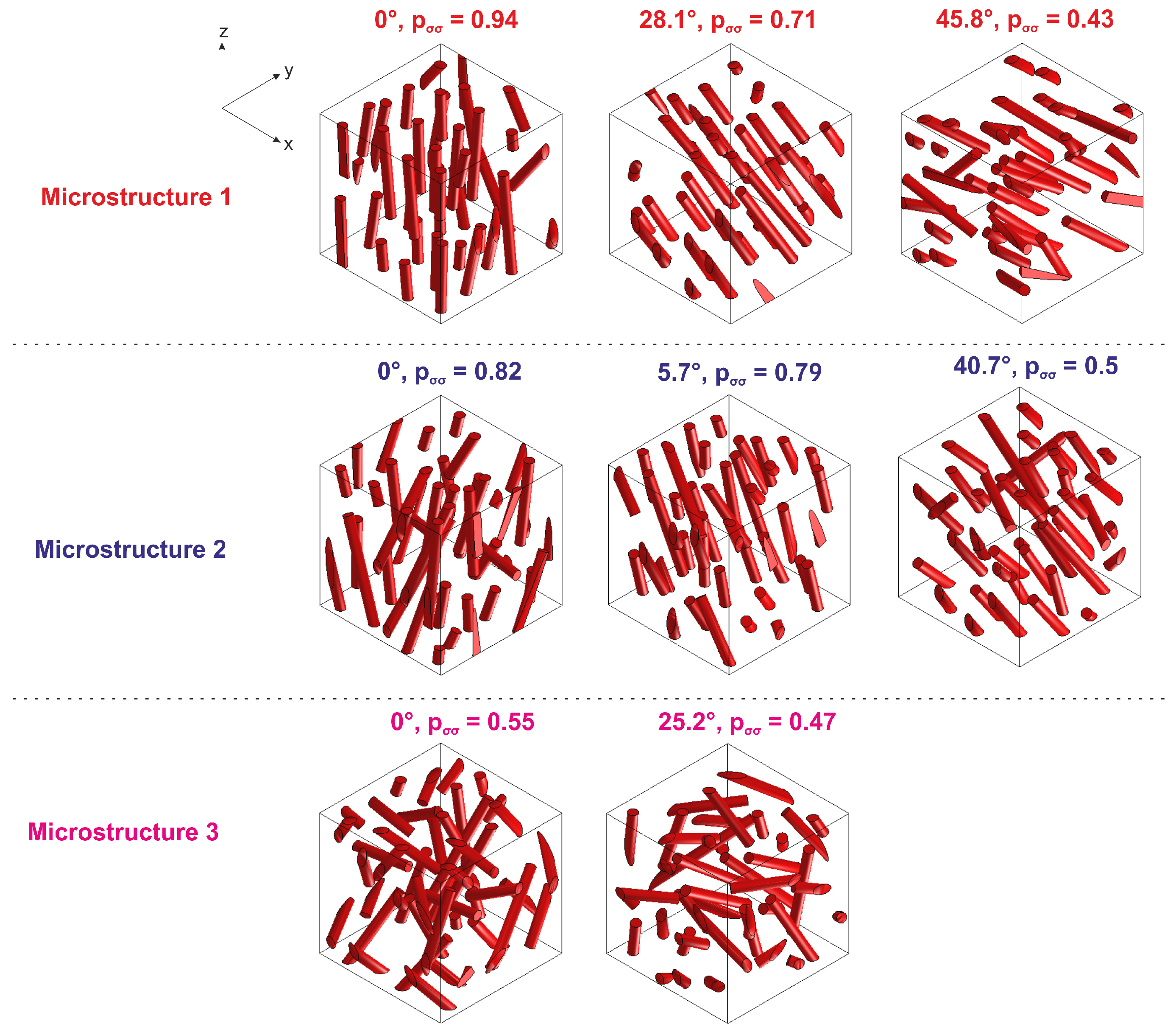
In this article, a transversely isotropic E-glass short-fiber-reinforced polycarbonate was considered with the third direction as the symmetry axis. Therefore, the diagonal components of the 3 by 3 fiber orientation tensor must satisfy , and the non-diagonal components are 0. Three transversely isotropic fiber orientation distributions, with , and were, respectively, introduced to represent three microstructures. Each microstructure is used to study the corresponding anisotropic behavior. Because of the limited number of fibers in a representative volume element, the desired transversely isotropic fiber orientation tensor is approximated with a tolerance of in each of its components.
Rotated microstructures are created based on the rotated fiber orientation tensors , as shown in Figure 2. In order to simplify the description of the fiber orientation, a fiber orientation factor is extracted from the rotated fiber orientation tensor and it represents the fiber orientation along the loading direction. When , all fibers are aligned with the loading direction and when , all fibers are perpendicular to the loading direction. In the results section, the orientation of the fiber is indicated by .
2.2. Periodic Boundary Condition
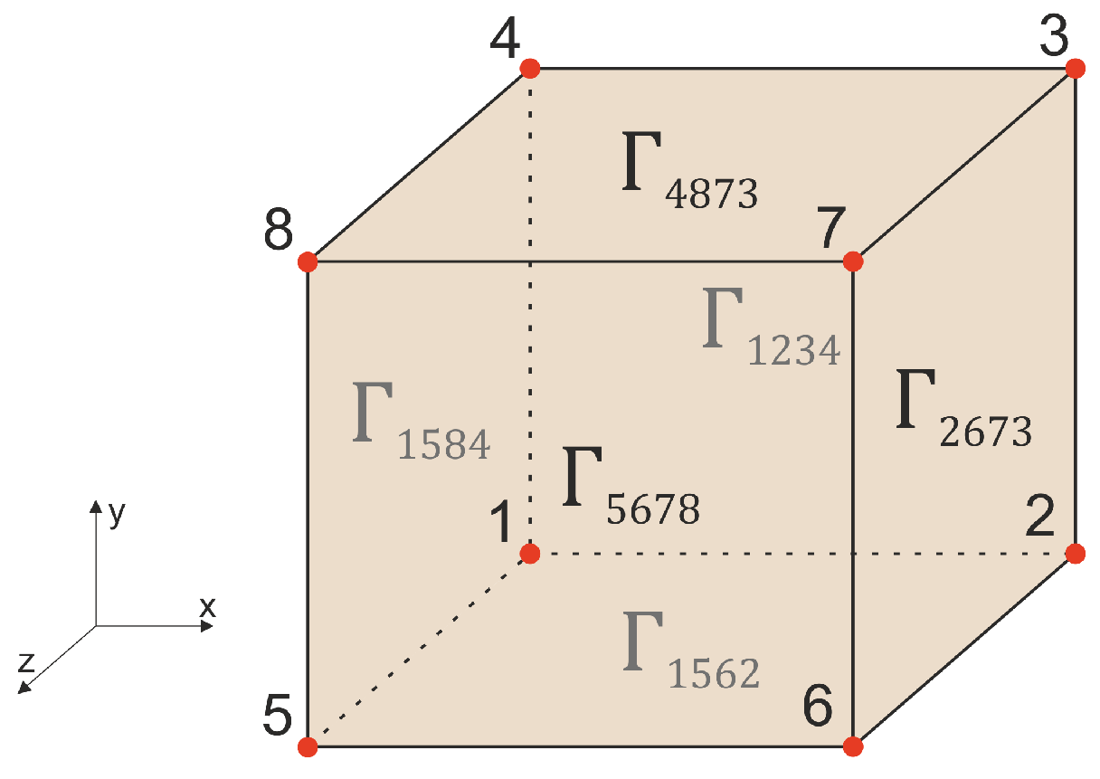
Periodic boundary conditions were applied to the periodic RVEs to homogenize the response of the heterogeneous materials [36]. The periodic boundary conditions ensure that the deformed shapes of two opposing faces remain identical. For this purpose, the boundary of the representative volume element is split into six boundary faces, here denoted as , , , , and (see Figure 3). The periodicity can then be formulated in terms of the displacements u of the nodes in the boundary faces and corner nodes:
The RVE is loaded with a uniaxial strain at a macroscopically constant strain rate by prescribing the displacement of corner node 5 as
where is the initial length of the RVE in the z direction. Additionally, the displacement of corner node 1 is suppressed in the x, y and z direction, the displacement of corner node 5 is suppressed in the x direction, the displacement of corner node 2 is suppressed in the z direction and the displacement of corner node 4 is suppressed in the y direction. The macroscopic first Piola–Kirchhoff stress tensor is obtained as
where is the reaction force and is the position vector of the corner nodes in the reference state. is the volume of the RVE in the reference state. The corresponding macroscopic Cauchy stress is then given by
where is the macroscopic deformation gradient, which is obtained as
with the outward normal of the boundary in the initial state.
2.3. The Strain Rate-Dependent EGP Model
The rate dependence of the E-glass short-fiber-reinforced polycarbonate stems from the rate-dependent polycarbonate matrix. The EGP model can accurately describe the strain rate-dependent visco-elastic regime, yield stress, strain softening and hardening of amorphous polymers and is used here to describe the polycarbonate matrix. The small strain behavior, including yield and strain softening, is determined by the inter-molecular interactions as a visco-elastic contribution. The larger strain behavior with the strain hardening is governed by the molecular network as a rubber-elastic contribution. Based on these two contributions, the total Cauchy stress is split into an elasto-viscoplastic driving stress and an elastic hardening stress :
The elastic and plastic parts of the total deformation are defined through a multiplicative decomposition of the deformation gradient tensor :
where the subscripts e and p refer to the elastic and plastic parts of the deformation, respectively.
For polycarbonate, two relaxation processes and exist. However, since the material is tested at room temperature and the strain rates are lower than , the process, which dominates at higher strain rates, is ignored [37]. Therefore, in order to save valuable computation time, the driving stress only represents the process:
where subscript k denotes the individual modes; n is the total number of modes; is the constant bulk modulus; is the volume change ratio; is the second-order unit tensor. and are, respectively, the shear modulus and the deviatoric part of the isochoric elastic left Cauchy–Green deformation tensor, which is defined as
The relation between the driving stress and the plastic rate of deformation is described by using a non-Newtonian flow rule:
where a scalar viscosity depends on the absolute temperature T, equivalent stress , pressure p and the state parameter S:
where is the initial viscosity associated with mode k, is the activation enthalpy, R is the universal gas constant, and is the pressure dependence. is the characteristic shear stress, defined as
where V is the shear equivalent activation volume associated with Boltzmann’s constant . The stress and temperature dependency are based on the Eyring theory. The equivalent stress and pressure p are defined as
The state parameter S, which incorporates the description of the intrinsic strain softening in a glassy polymer, can be written as a function of the equivalent plastic strain :
where the initial state parameter represents the thermo-mechanical (aging) history of the material. Intrinsic strain softening is described by a modified version of the Carreau–Yasuda function :
with fit parameters , and .
The elastic hardening stress is obtained using the neo-Hookean expression:
where is the strain hardening modulus and .
All micromechanical simulations are conducted in Marc.Mentat 2014.0.0. The EGP model is implemented in a user-defined subroutine HYPELA2. The material parameters for the polycarbonate matrix are adopted from a previous study [33] (see Table A1 Appendix A). In Table A2 Appendix A, the reference spectrum for the polycarbonate matrix is shown with 17 modes.
3. Results and Discussions
Using direct finite element simulations, the homogenized stress–strain responses of RVEs, generated from specific fiber orientation tensors, are obtained. The RVE is meshed with 512,000 linear elements, and the FEA of the RVE is conducted with eight CPUs and 52 GB RAM. The computational running time until the yield point depends on the loading angle, since a finer time increment is required at lower loading angles for better convergence. In general, the computational running time until the yield point is 3 days at lower loading angles and less than 1 day at higher loading angles. To investigate the effect of different RVEs with identical orientation distributions, four RVEs were generated with (see Figure 4a). The simulated stress–strain curves of these RVEs are presented in Figure 4b for loading angles of and at a strain rate of . The yield point is obtained as the maximum stress of the stress–strain curve, which is presented as the marker in Figure 4b. The observed variation is clearly small; for the loading angle, the stress–strain curves for the different RVEs are almost indistinguishable as they are on top of one another. In the direction, where changes in fiber placement may be expected to have a larger influence, the yield stress variation is still very small, MPa ± MPa, i.e., a variation of little more than . These small variations between RVEs are a strong indication that the RVE size is large enough and can indeed be regarded as representative.
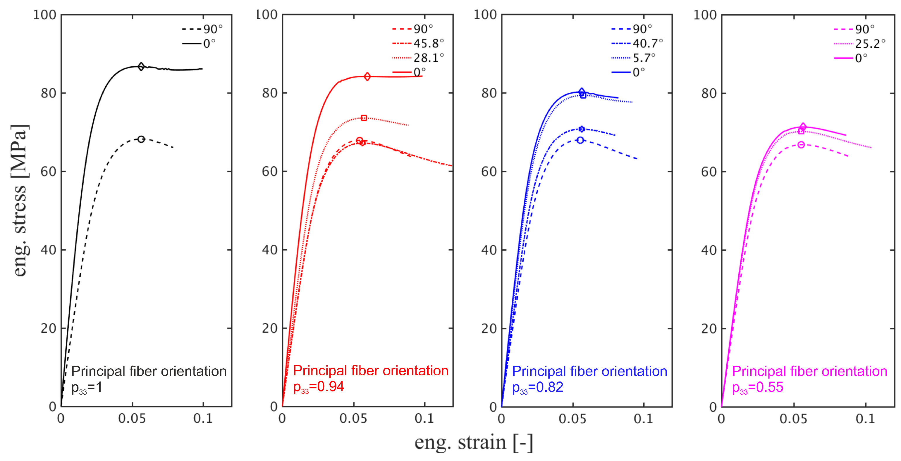
To investigate the influence of fiber orientation on the mechanical response, further simulations were performed at a strain rate of for different values of the principal fiber orientation and various loading angles. The RVEs used were presented in Figure 2. Illustrative examples of the simulated stress–strain curves are shown in Figure 5, where it is clear that the fiber orientation, as well as the loading angle both markedly influence the mechanical response. Upon a decrease in value of , a gradual decrease in the yield stress and elastic modulus is observed in the loading direction. A similar change in stress–strain response is observed when the loading angle increases gradually from to , where it should be noted that the value of the principal fiber orientation has almost no influence on the response in the loading direction. Even in the moderate case studied here, a composite with a fiber loading of weight fraction, a clear orientation-induced anisotropy is observed.
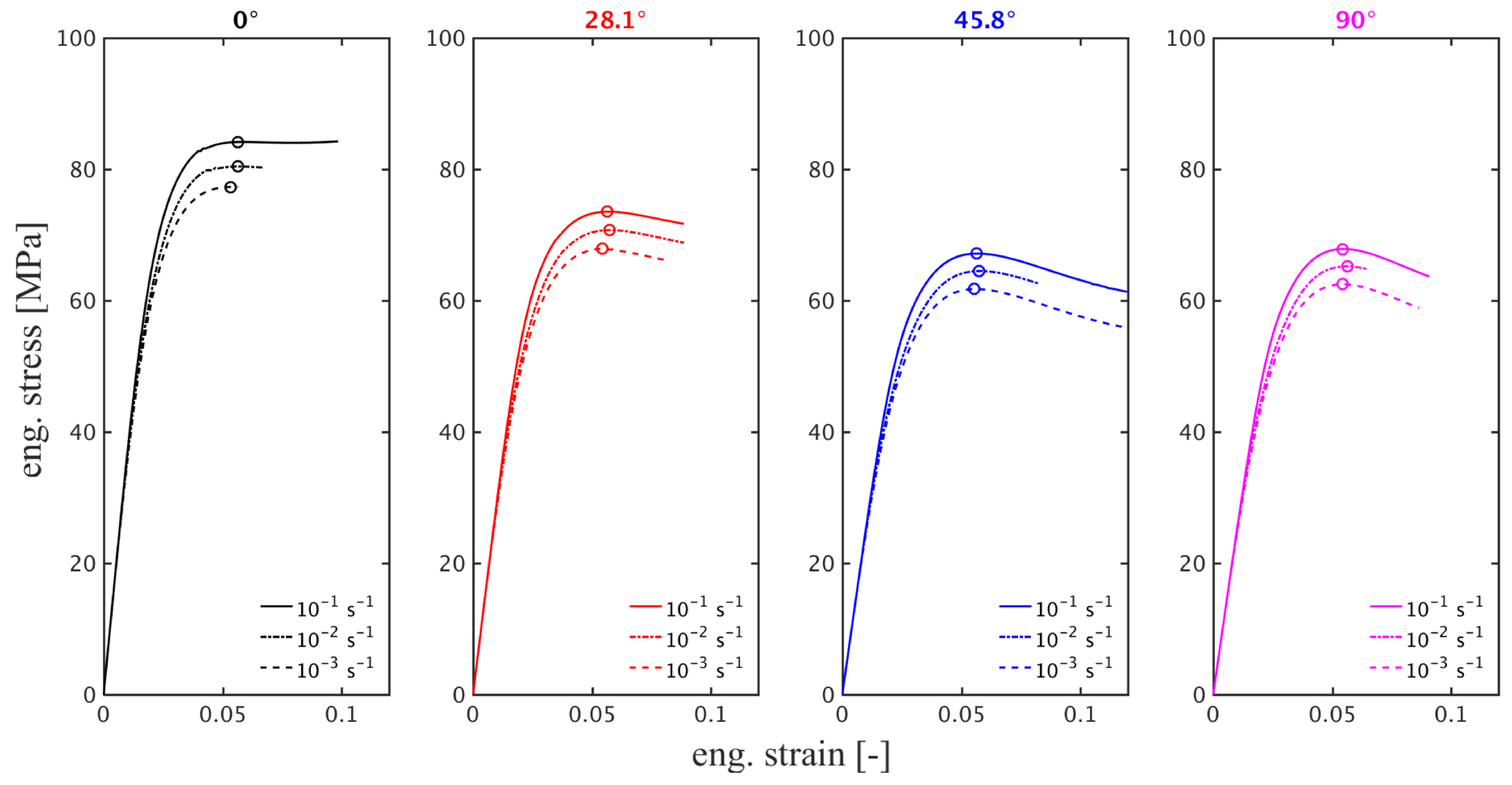
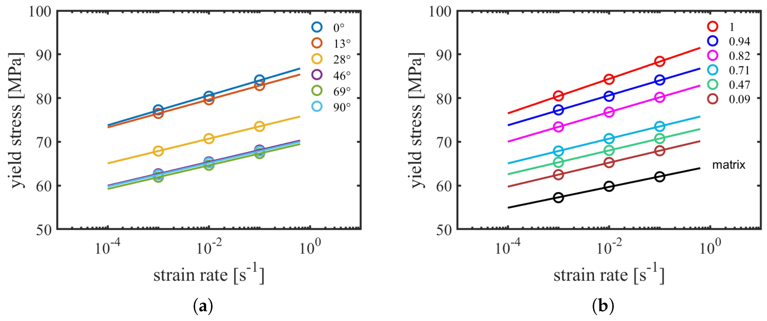
Since the matrix material displays a significant dependence on the applied strain rate, the results of simulations at various strain rates on a representative volume element with are presented in Figure 6, for various loading angles. Some curves end earlier because their simulations were manually terminated earlier after the yield (maximum) stress was reached. Meanwhile, some simulations indeed stop earlier due to the non-convergence, especially at lower loading angles. The resulting yield stresses at the different strain rates were determined and are presented in Figure 7a in a semi-log representation of yield stress versus the logarithm of strain rate. Figure 7a visualizes the pronounced influence of loading angle on the value of the yield stress. Additionally, the results seem to indicate that the strain rate dependence of the yield stress, here quantified as the slope of the lines (guides to the eye), also displays a variation with the loading angle. To study this effect in more detail, extra simulations were performed on RVEs with -values of , , , , and , for a loading angle of (). The resulting yield stress values, at various strain rates, are presented in Figure 7b, where the response of the unfilled matrix is also added. With the larger range in fiber orientation, its influence on the strain rate dependence of the yield stress is clearly more pronounced. The trend becomes clearer when the values of the simulated strain rate dependence are ranked with respect to increasing , the fiber orientation in the direction of loading. These are presented in Table 1, which shows that, initially, up to a of , the slope only changes marginally, and stays more or less constant. At larger fiber orientations, there is a marked increase in the strain rate dependence with increasing . A similar trend is observed in the yield stress which also shows a marked increase at larger values.
The observed trends appear in good agreement with experimental observations of glass fiber-reinforced polycarbonate [10,12,13,14]. In these experimental studies, it was demonstrated that the influence of loading angle/fiber orientation and strain rate dependence are, to a good approximation, factorizable—implying that the influence of the strain rate and that of the loading angle are actually decoupled. This was shown by plotting the yield stress data versus strain rate in a double logarithmic plot. This procedure yielded parallel lines, demonstrating that the influence of fiber orientation and that of strain rate can be separated in a multiplicative manner. This factorizability was not only observed for the low fiber weight fraction used in this study, but also for other fiber-reinforced systems with fiber weight fractions and aspect ratios over the entire range commercially available.
As shown in Figure 8a,b, presenting the double logarithmic versions of the semi-log plots presented in Figure 7a,b, a similar observation can be made. For different fiber orientations, the strain rate dependence of the simulated yield stresses, to a good approximation, is also transformed to a set of parallel lines. Remarkably, the simulated response of the unreinforced matrix seems to fit this trend well, clearly witnessing that the polymer matrix is the origin of the observed rate dependence, and that the effect of fiber-reinforcement and orientation merely shifts the response—a geometrical effect which can be identified by micromechanical simulations.
In practical terms, the results presented in Figure 8 imply that the dependence of the yield stress on strain rate and loading angle can be expressed as
For a logarithmic stress-axis, the multiplicative decoupling transforms into:
where represents the strain rate dependence of the yield stress for a chosen reference state, the loading angle , which is generally chosen to be . To obtain a suitable expression for , the Hill equivalent stress, based on the well-known Hill yield function [38] is used. To simplify the expression, a plane stress state was assumed, in which case:
with:
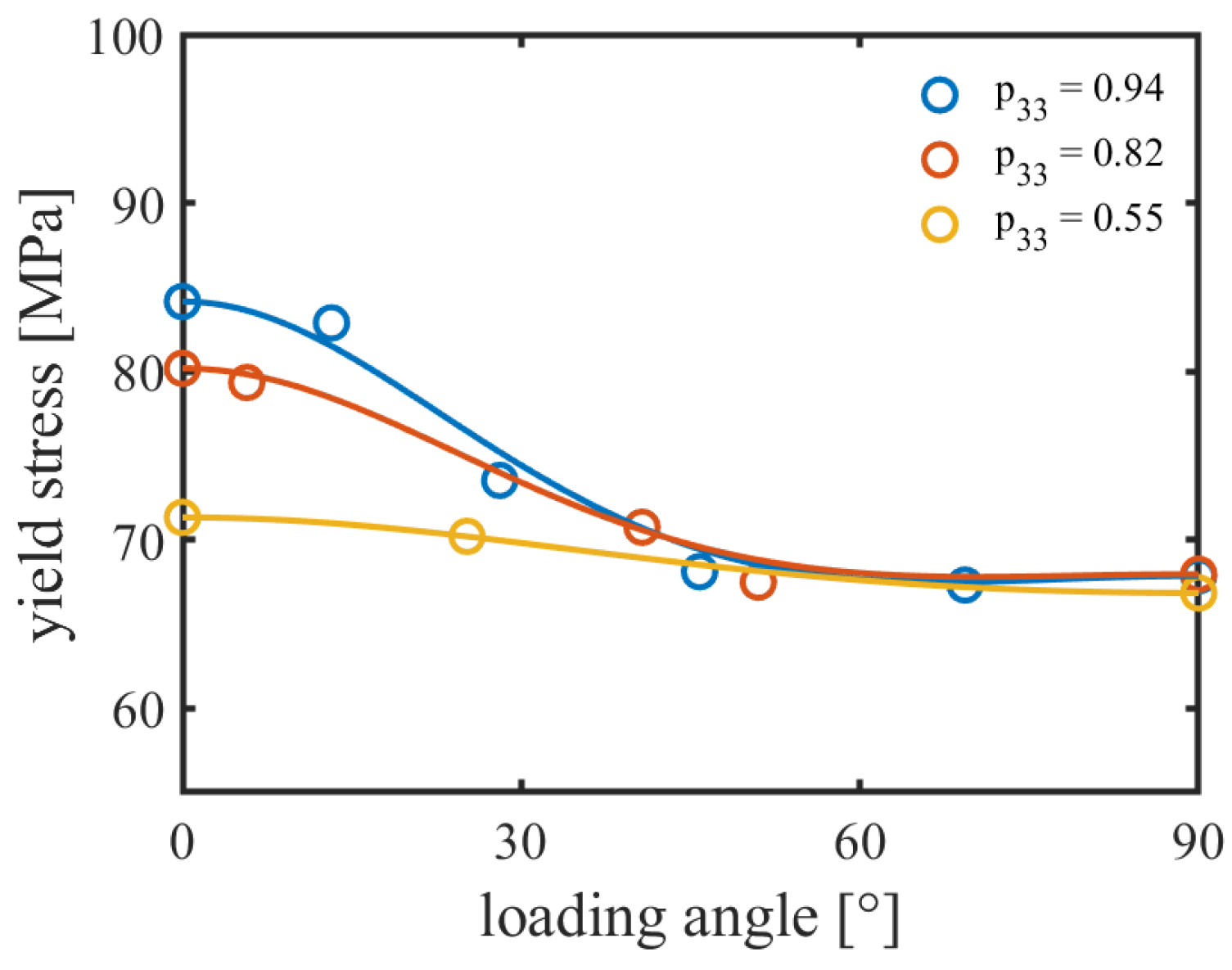
where the constants , and are ratios of the yield stress in different principal material orientations to the reference yield stress . The value of is the ratio of the shear yield stress to the reference shear yield stress . In our specific case, it should be noted that the R-values are all independent of strain rate. Since strain rate and loading angle dependence are decoupled, the latter are determined at an (arbitrarily chosen) strain rate. An example of the application of the Hill equivalent stress approach is shown in Figure 9, which presents the loading angle dependence at a strain rate of for a principal fiber orientation of , and . The solid lines are fits with Equations (19) and (21), taking the yield stress at as a reference yield stress. It is clear that the Hill function adequately represents the observed loading angle dependence. The Hill parameters obtained from the fit are presented in Table 2.
Figure 9 clearly demonstrates the strong influence of fiber orientation on local anisotropy; a different fiber orientation distribution clearly reflects marked changes of the load angle dependence. Of course, in a realistic situation, where a complex shaped component is injection-molded, the variation in the flow conditions over the product shape will lead to a pronounced spatial variation of the local fiber orientation throughout the product. Simultaneously, this implies that the anisotropic mechanical response will demonstrate a similar spatial variation. This variation of properties throughout the product, and its complex relation to processing conditions, product geometry, flow and mechanical characteristics of the fiber-reinforced polymer is one of the major challenges encountered in the design of load-bearing fiber-reinforced polymer components today. The usual approach is to address the problem in a two steps; firstly, a simulation of the processing step, in which the designer can obtain information on the local fiber orientation distribution throughout the component. Methods to achieve this were developed over the years [34,39,40], and are readily available in various commercial software packages dedicated to injection molding. The second step is the translation of the local fiber orientation distribution to the resulting, local, anisotropic mechanical response. This step is complex, since it usually involves either a mean-field homogenization such as Mori–Tanaka model or a full-field homogenization through the FEA of RVEs. The mean-field homogenization was able to rapidly provide the overall response and is commonly used for actual product simulations. Meanwhile, the full-field homogenization provides a better accuracy and is used in the current study. From these, the local parameters of a suitable macroscopic constitutive model must be determined, leading to a set of parameters that may vary from element to element.
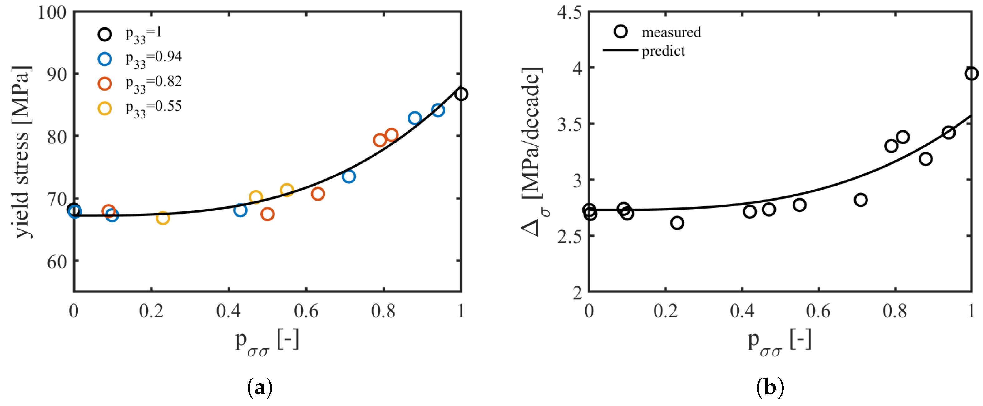
The results from our simulations, however, also reveal the possibility of an alternative route. From Figure 8a, it became evident that, as mathematically defined in Equation (19), the dependence of the yield stress on strain rate and loading angle are multiplicatively decoupled. This implies that the rate dependence can be characterized on a reference orientation of choice. Figure 8b additionally evidences that the same rate dependence is actually applicable over a great variety of , obtained from different orientation distributions tested in various loading directions. Hence, it appears interesting to investigate how the value of influences the value of the yield stress at a single strain rate. The result is presented in Figure 10a, for a strain rate of , and demonstrates that the yield stress is intimately related to the fiber orientation in loading direction . A similar observation was also experimentally made on a polycarbonate composite system with weight fraction of short glass fibers, although in the experimental case, the range of fiber orientations was more limited () [14]. The observed trend is described well by
where is the reference strain rate chosen ( in this case), is the reference orientation chosen to determine the rate dependence (most obvious choice ), and and q are parameters to be determined by fitting. As can be observed in Figure 10a, a satisfactory fit is obtained with MPa and .
Equivalent to Equation (19), it is convenient to rewrite Equation (23) to
where, following Equation (23):
and can be described using an Eyring expression, in the isothermal case simplified to:
which provides the linear relationship between the yield stress and the logarithm of strain rate that is generally observed over large ranges of strain rate and temperature [10]. On a log base 10 scale, the slope of the reference orientation can be expressed as
Of course, with increasing fiber orientation, the slope will also gradually increase, and from Equation (24), it can easily be deduced that this can be expressed as
with defined by Equation (25). With all the parameters required determined from Figure 10a, Figure 10b presents a direct comparison between the measured slopes for different , listed in Table 1, and the trend that is predicted by Equation (28). Overall, the deviations are in the order of , except for the perfectly aligned case.
The results in Figure 10 suggest that, with adequate material characterization, expressions can be found that conveniently link the yield stress and its strain rate dependence to the fiber orientation in the direction of loading. Such a relation can be employed to create direct analytical links between the local fiber orientation distribution (as obtained from injection molding simulations) and the parameters required for the characterization of its anisotropic macroscopic response (Hill parameters, rate dependence).
4. Conclusions
In this study, we employed a straightforward micromechanical modeling approach to study the anisotropy in the strain rate dependence of the mechanical response of a short (glass) fiber-reinforced polycarbonate. The matrix response was captured using the EGP-model, which was shown earlier to accurately represent the rate-dependent mechanical response of polycarbonate [33], and the glass fibers were modeled as linear elastic solids. RVEs were generated based on several transversely isotropic orientation distributions of short glass fibers with fixed length. The results of the simulations demonstrate that the influence of the loading direction and that of the strain rate can be regarded independently (factorizable), and that they are multiplicatively decoupled. This implies that the rate dependence of the system can be fully characterized in a single (reference) loading angle and the dependence on loading direction at a single strain rate. Moreover, the results also clearly demonstrate that the yield stress, to a good approximation, can be directly linked to the fiber orientation in the direction of loading. This leads to a new relation that uniquely links the rate dependence of the yield stress to the fiber orientation in the loading direction. We expect that the observed multiplicative decoupling can be the basis of a novel method to rapidly estimate the anisotropic mechanical response of short-fiber-reinforced thermoplastics on the basis of fiber orientation distribution. Such a method would be invaluable with respect to the development of new predictive methodologies that can take processing-induced fiber orientation into account in the very early stages of design of load-bearing components.
For future work, the micromechanical modeling in this study could be extended from an amorphous to a semicrystalline polymer matrix, since a considerable amount of polymer composites are based on semicrystalline polymers. It has been shown that the modular set-up of the EGP model provides a versatile tool that can also be successfully applied to semicrystalline polymers [41].
Author Contributions
Conceptualization, S.Z., L.E.G. and J.A.W.v.D.; methodology, S.Z., L.E.G. and J.A.W.v.D.; validation, S.Z.; formal analysis, S.Z.; investigation, S.Z.; data curation, S.Z.; writing—original draft preparation, S.Z.; writing—review and editing, L.E.G. and J.A.W.v.D.; visualization, S.Z.; supervision, L.E.G. and J.A.W.v.D.; project administration, L.E.G. and J.A.W.v.D.; funding acquisition, L.E.G. and J.A.W.v.D. All authors have read and agreed to the published version of the manuscript.
Funding
This research was funded by Saudi Basic Industries Corporation.
Institutional Review Board Statement
Not applicable.
Informed Consent Statement
Not applicable.
Data Availability Statement
The data generated or analyzed in this study are available upon reasonable request.
Acknowledgments
The authors gratefully acknowledge financial support by SABIC and thank Tim van Erp for stimulating discussions.
Conflicts of Interest
The authors declare no conflict of interest. The funders had no role in the design of the study; in the collection, analyses, or interpretation of data; in the writing of the manuscript, or in the decision to publish the results.
Appendix A

Table A1.
Material parameters for polycarbonate matrix [33].
Table A1.
Material parameters for polycarbonate matrix [33].
| (MPa) | (MPa) | (MPa) | (-) | (-) | (-) | (-) | (-) |
|---|---|---|---|---|---|---|---|
| 26 | 3750 | 28 | 50 |
Table A2.
Reference spectrum for polycarbonate matrix [33].
Table A2.
Reference spectrum for polycarbonate matrix [33].
| Modes | (MPa) | (MPa · s) |
|---|---|---|
| 1 | ||
| 2 | ||
| 3 | ||
| 4 | ||
| 5 | ||
| 6 | ||
| 7 | ||
| 8 | ||
| 9 | ||
| 10 | ||
| 11 | ||
| 12 | ||
| 13 | ||
| 14 | ||
| 15 | ||
| 16 | ||
| 17 |
References
- Ishikawa, T.; Amaoka, K.; Masubuchi, Y.; Yamamoto, T.; Yamanaka, A.; Arai, M.; Takahashi, J. Overview of automotive structural composites technology developments in Japan. Compos. Sci. Technol. 2018, 155, 221–246. [Google Scholar] [CrossRef]
- Bernasconi, A.; Cosmi, F.; Hine, P.J. Analysis of fibre orientation distribution in short fibre reinforced polymers: A comparison between optical and tomographic methods. Compos. Sci. Technol. 2012, 72, 2002–2008. [Google Scholar] [CrossRef]
- Kim, E.G.; Park, J.K.; Jo, S.H. A study on fiber orientation during the injection molding of fiber-reinforced polymeric composites: (Comparison between image processing results and numerical simulation). J. Mater. Process. Technol. 2001, 111, 225–232. [Google Scholar] [CrossRef]
- Sedighiamiri, A.; van Erp, T.; Cathelin, J.; Brands, D. Validation methodology for accurate prediction of anisotropic mechanics in fiber reinforced thermoplastic (FRTP) materials. In Proceedings of the 20th International Conference on Composite Materials, Copenhagen, Denmark, 19–24 July 2015. [Google Scholar]
- Davies, R.G.; Magee, C.L. The effect of strain-rate upon the tensile deformation of materials. J. Eng. Mater. Technol. 1975, 97, 151–155. [Google Scholar] [CrossRef]
- Okoli, O.I. The effects of strain rate and failure modes on the failure energy of fibre reinforced composites. Compos. Struct. 2001, 54, 299–303. [Google Scholar] [CrossRef]
- Vashchenko, A.; Spiridonova, I.; Sukhovaya, E. Deformation and fracture of structural materials under high-rate strain. Metalurgija 2000, 39, 89–92. [Google Scholar]
- Li, R.K.Y.; Lu, S.N.; Choy, C.L. Tensile and compressive deformation of a short-glass-fiber-reinforced liquid crystalline polymer. J. Thermoplast. Compos. Mater. 1995, 8, 304–322. [Google Scholar] [CrossRef] [Green Version]
- Goldberg, R.K.; Stouffer, D.C. Strain rate dependent analysis of a polymer matrix composite utilizing a micromechanics approach. J. Compos. Mater. 2002, 36, 773–793. [Google Scholar] [CrossRef]
- Govaert, L.E.; van der Vegt, A.K.; van Drongelen, M. Polymers: From Structure to Properties; Delft Academic Press: Delft, The Netherlands, 2020; Chapter 7. [Google Scholar]
- Loo, L.S.; Cohen, R.E.; Gleason, K.K. Chain mobility in the amorphous region of nylon 6 observed under active uniaxial deformation. Science 2000, 288, 116–119. [Google Scholar] [CrossRef]
- Pastukhov, L.V.; and Govaert, L.E. Plasticity-controlled failure of fibre-reinforced thermoplastics. Compos. Part B Eng. 2021, 209, 108635. [Google Scholar] [CrossRef]
- Pastukhov, L.V.; Kanters, M.J.; Engels, T.A.; Govaert, L.E. Influence of fiber orientation, temperature and relative humidity on the long-term performance of short glass fiber reinforced polyamide 6. J. Appl. Polym. Sci. 2021, 138, 50382. [Google Scholar] [CrossRef]
- Amiri-Rad, A.; Wismans, M.; Pastukhov, L.V.; Govaert, L.E.; van Dommelen, J.A.W. Constitutive modeling of injection-molded short-fiber composites: Characterization and model application. J. Appl. Polym. Sci. 2020, 137, 49248. [Google Scholar] [CrossRef]
- Benveniste, Y. A new approach to the application of Mori-Tanaka’s theory in composite materials. Mech. Mater. 1987, 6, 147–157. [Google Scholar] [CrossRef]
- Mori, T.; Tanaka, K. Average stress in matrix and average elastic energy of materials with misfitting inclusions. Acta Metall. 1973, 21, 571–574. [Google Scholar] [CrossRef]
- Camacho, C.W.; Tucker, C.L., III; Yalvaç, S.; McGee, R.L. Stiffness and thermal expansion predictions for hybrid short fiber composites. Polym. Compos. 1990, 11, 229–239. [Google Scholar] [CrossRef]
- Lusti, H.R.; Gusev, A.A. Finite element predictions for the thermoelastic properties of nanotube reinforced polymers. Model. Simul. Mater. Sci. Eng. 2004, 12, S107. [Google Scholar] [CrossRef]
- Pierard, O.; Friebel, C.; Doghri, I. Mean-field homogenization of multi-phase thermo-elastic composites: A general framework and its validation. Compos. Sci. Technol. 2004, 64, 1587–1603. [Google Scholar] [CrossRef]
- Krairi, A.; Doghri, I.; Robert, G. Multiscale high cycle fatigue models for neat and short fiber reinforced thermoplastic polymers. Int. J. Fatigue 2016, 92, 179–192. [Google Scholar] [CrossRef]
- Yim, S.O.; Lee, W.J.; Cho, D.H.; Park, I.M. Finite element analysis of compressive behavior of hybrid short fiber/particle/mg metal matrix composites using RVE model. Met. Mater. Int. 2015, 21, 408–414. [Google Scholar] [CrossRef]
- Mortazavi, B.; Baniassadi, M.; Bardon, J.; Ahzi, S. Modeling of two-phase random composite materials by finite element, Mori–Tanaka and strong contrast methods. Compos. Part B Eng. 2013, 45, 1117–1125. [Google Scholar] [CrossRef]
- Ali, D.; Sen, S. Finite element analysis of the effect of boron nitride nanotubes in beta tricalcium phosphate and hydroxyapatite elastic modulus using the RVE model. Compos. Part B Eng. 2016, 90, 336–340. [Google Scholar] [CrossRef]
- Goldberg, R.K.; Roberts, G.D.; Gilat, A. Implementation of an associative flow rule including hydrostatic stress effects into the high strain rate deformation analysis of polymer matrix composites. J. Aerosp. Eng. 2005, 18, 18–27. [Google Scholar] [CrossRef]
- Tabiei, A.; Aminjikarai, S.B. A strain-rate dependent micro-mechanical model with progressive post-failure behavior for predicting impact response of unidirectional composite laminates. Compos. Struct. 2009, 88, 65–82. [Google Scholar] [CrossRef]
- Haward, R.N.; Thackray, G. The use of a mathematical model to describe isothermal stress–strain curves in glassy thermoplastics. Proc. R. Soc. Lond. Ser. A Math. Phys. Sci. 1968, 302, 453–472. [Google Scholar]
- Boyce, M.C.; Parks, D.M.; Argon, A.S. Large inelastic deformation of glassy polymers. Part I: rate dependent constitutive model. Mech. Mater. 1988, 7, 15–33. [Google Scholar] [CrossRef]
- Arruda, E.M.; Boyce, M.C. Evolution of plastic anisotropy in amorphous polymers during finite straining. Int. J. Plast. 1993, 9, 697–720. [Google Scholar] [CrossRef]
- Hasan, O.A.; Boyce, M.C.; Li, X.S.; Berko, S. An investigation of the yield and postyield behavior and corresponding structure of poly (methyl methacrylate). J. Polym. Sci. Part B Polym. Phys. 1993, 31, 185–197. [Google Scholar] [CrossRef]
- Buckley, C.P.; Jones, D.C. Glass-rubber constitutive model for amorphous polymers near the glass transition. Polymer 1995, 36, 3301–3312. [Google Scholar] [CrossRef]
- Buckley, C.P.; Dooling, P.J.; Harding, J.; Ruiz, C. Deformation of thermosetting resins at impact rates of strain. Part 2: Constitutive model with rejuvenation. J. Mech. Phys. Solids 2004, 52, 2355–2377. [Google Scholar] [CrossRef]
- Klompen, E.T.J.; Engels, T.A.P.; Govaert, L.E.; Meijer, H.E.H. Modeling of the postyield response of glassy polymers: Influence of thermomechanical history. Macromolecules 2005, 38, 6997–7008. [Google Scholar] [CrossRef] [Green Version]
- van Breemen, L.C.A.; Klompen, E.T.J.; Govaert, L.E.; Meijer, H.E.H. Extending the EGP constitutive model for polymer glasses to multiple relaxation times. J. Mech. Phys. Solids 2011, 59, 2191–2207. [Google Scholar] [CrossRef]
- Advani, S.G.; Tucker, C.L., III. The use of tensors to describe and predict fiber orientation in short fiber composites. J. Rheol. 1987, 31, 751–784. [Google Scholar] [CrossRef]
- Digimat, The Material Modeling Platform. Available online: https://www.e-xstream.com/ (accessed on 25 May 2021).
- Kouznetsova, V.G.; Geers, M.G.D.; Brekelmans, W.A.M. Multi-scale second-order computational homogenization of multi-phase materials: A nested finite element solution strategy. Comput. Methods Appl. Mech. Eng. 2004, 193, 5525–5550. [Google Scholar] [CrossRef]
- Bauwens-Crowet, C.; Bauwens, J.C.; Homes, G. The temperature dependence of yield of polycarbonate in uniaxial compression and tensile tests. J. Mater. Sci. 1972, 7, 176–183. [Google Scholar] [CrossRef]
- Hill, R. A theory of the yielding and plastic flow of anisotropic metals. Proc. R. Soc. Lond. Ser. A Math. Phys. Sci. 1948, 193, 281–297. [Google Scholar]
- Bay, R.S.; Tucker, C.L., III. Fiber orientation in simple injection moldings. Part I: Theory and numerical methods. Polym. Compos. 1992, 13, 317–331. [Google Scholar] [CrossRef]
- Bay, R.S.; Tucker, C.L., III. Fiber orientation in simple injection moldings. Part II: Experimental results. Polym. Compos. 1992, 13, 332–341. [Google Scholar] [CrossRef]
- Van Breemen, L.C.A.; Engels, T.A.P.; Klompen, E.T.J.; Senden, D.J.A.; Govaert, L.E. Rate-and temperature-dependent strain softening in solid polymers. J. Polym. Sci. Part B Polym. Phys. 2012, 50, 1757–1771. [Google Scholar] [CrossRef]
Figure 1.
A schematic work flow for investigating the anisotropic and rate-dependent behavior of short-fiber-reinforced thermoplastics.
Figure 1.
A schematic work flow for investigating the anisotropic and rate-dependent behavior of short-fiber-reinforced thermoplastics.

Figure 2.
Microstructures 1, 2 and 3 are rotated at various angles with respect to the loading direction. At each angle, the fiber orientation factor corresponding to loading in the z direction is illustrated.
Figure 2.
Microstructures 1, 2 and 3 are rotated at various angles with respect to the loading direction. At each angle, the fiber orientation factor corresponding to loading in the z direction is illustrated.

Figure 3.
The definition of the boundary corners and surfaces. The red markers represent the corner nodes 1–8. The left and right boundary surfaces are and . The top and bottom boundary faces are and . The front and back boundary faces are and .
Figure 3.
The definition of the boundary corners and surfaces. The red markers represent the corner nodes 1–8. The left and right boundary surfaces are and . The top and bottom boundary faces are and . The front and back boundary faces are and .

Figure 4.
(a) Four different RVEs containing weight fraction of glass fibers with an aspect ratio of 12 and a principal fiber orientation ; (b) simulated stress–strain curves for each RVE for loading angles of and at a strain rate of . Markers indicate yield stress.
Figure 4.
(a) Four different RVEs containing weight fraction of glass fibers with an aspect ratio of 12 and a principal fiber orientation ; (b) simulated stress–strain curves for each RVE for loading angles of and at a strain rate of . Markers indicate yield stress.

Figure 5.
Simulated stress–strain curves for a strain rate of , using RVEs with principal fiber orientations of 1, , and . For each principal fiber orientation, the stress–strain curve is obtained for various loading angles. Markers indicate yield stress.
Figure 5.
Simulated stress–strain curves for a strain rate of , using RVEs with principal fiber orientations of 1, , and . For each principal fiber orientation, the stress–strain curve is obtained for various loading angles. Markers indicate yield stress.

Figure 6.
Illustration of the strain rate dependence observed in an RVE with a principal fiber orientation = 0.94. Figures present simulated stress–strain curves in various loading directions and for strain rates. Markers indicate yield stress.
Figure 6.
Illustration of the strain rate dependence observed in an RVE with a principal fiber orientation = 0.94. Figures present simulated stress–strain curves in various loading directions and for strain rates. Markers indicate yield stress.

Figure 7.
(a) Semi–log plot of the strain rate dependence of the simulated yield stress of an RVE with a principal fiber orientation for different loading angles; and (b) semi–log plot of the strain rate dependence of the simulated yield stress of RVEs with various fiber orientation and the unreinforced matrix. Markers are simulation results; lines represent guides to the eye.

Figure 8.
(a) Log–log plot of the strain rate dependence of the simulated yield stress of an RVE with a principal fiber orientation of for different loading angles; and (b) log–log plot of the strain rate dependence of the simulated yield stress of RVEs with various fiber orientation . Markers are simulation results; lines are perfectly parallel and represent guides to the eye. Black line and markers correspond to the response of the unreinforced matrix.

Figure 9.
Loading angle dependence of the yield stress at a strain rate of for different principal fiber orientations. Markers are simulation results; lines are fits using the Hill yield function.
Figure 9.
Loading angle dependence of the yield stress at a strain rate of for different principal fiber orientations. Markers are simulation results; lines are fits using the Hill yield function.

Figure 10.
(a) Simulated yield stress at (markers), plotted versus the fiber orientation in the direction of loading . Each color represents the results obtained for a specific principal fiber orientation under different loading angles. Lines are fits according to Equation (23), using the parameters listed in the text; (b) simulated slope (rate dependence of yield stress) at (markers) versus the fiber orientation in the direction of loading . The line is the prediction from the reference orientation through Equation (28).

Table 1.
Simulated values of yield stress and rate dependence of the yield stress in a semi-log plot for different fiber orientations.
Table 1.
Simulated values of yield stress and rate dependence of the yield stress in a semi-log plot for different fiber orientations.
| Principal Orientation (-) | Loading Angle () | Orientation in Loading Direction (-) | Rate Dependence of Yield Stress (MPa/Decade) | Yield Stress@ (MPa) |
|---|---|---|---|---|
| matrix | isotropic | - | ||
| 1 | 90 | 0 | ||
| 90 | ||||
| 90 | ||||
| 69 | ||||
| 90 | ||||
| 46 | ||||
| 25 | ||||
| 0 | ||||
| 41 | ||||
| 28 | ||||
| 6 | ||||
| 0 | ||||
| 0 | ||||
| 1 | 0 | 1 |
Table 2.
Hill parameters obtained from Figure 9.
Table 2.
Hill parameters obtained from Figure 9.
| (-) | (MPa) | (-) | (-) | (-) |
|---|---|---|---|---|
| 1 | ||||
| 1 | ||||
| 1 |
Publisher’s Note: MDPI stays neutral with regard to jurisdictional claims in published maps and institutional affiliations. |
© 2021 by the authors. Licensee MDPI, Basel, Switzerland. This article is an open access article distributed under the terms and conditions of the Creative Commons Attribution (CC BY) license (https://creativecommons.org/licenses/by/4.0/).
Share and Cite
MDPI and ACS Style
Zhang, S.; van Dommelen, J.A.W.; Govaert, L.E. Micromechanical Modeling of Anisotropy and Strain Rate Dependence of Short-Fiber-Reinforced Thermoplastics. Fibers 2021, 9, 44. https://0-doi-org.brum.beds.ac.uk/10.3390/fib9070044
AMA Style
Zhang S, van Dommelen JAW, Govaert LE. Micromechanical Modeling of Anisotropy and Strain Rate Dependence of Short-Fiber-Reinforced Thermoplastics. Fibers. 2021; 9(7):44. https://0-doi-org.brum.beds.ac.uk/10.3390/fib9070044
Chicago/Turabian StyleZhang, Shaokang, Johannes A. W. van Dommelen, and Leon E. Govaert. 2021. "Micromechanical Modeling of Anisotropy and Strain Rate Dependence of Short-Fiber-Reinforced Thermoplastics" Fibers 9, no. 7: 44. https://0-doi-org.brum.beds.ac.uk/10.3390/fib9070044
Note that from the first issue of 2016, this journal uses article numbers instead of page numbers. See further details here.