
Optimal Asynchronous Dynamic Policies in Energy-Efficient Data Centers


1
Business School, Xuzhou University of Technology, Xuzhou 221018, China
2
School of Economics and Management, Beijing University of Technology, Beijing 100124, China
3
School of Business, Sun Yat-sen University, Guangzhou 510275, China
*
Author to whom correspondence should be addressed.
Systems 2022, 10(2), 27; https://0-doi-org.brum.beds.ac.uk/10.3390/systems10020027
Submission received: 24 January 2022
/
Revised: 26 February 2022
/
Accepted: 28 February 2022
/
Published: 2 March 2022
(This article belongs to the Special Issue Data Driven Decision-Making for Complex Production Systems)
Abstract
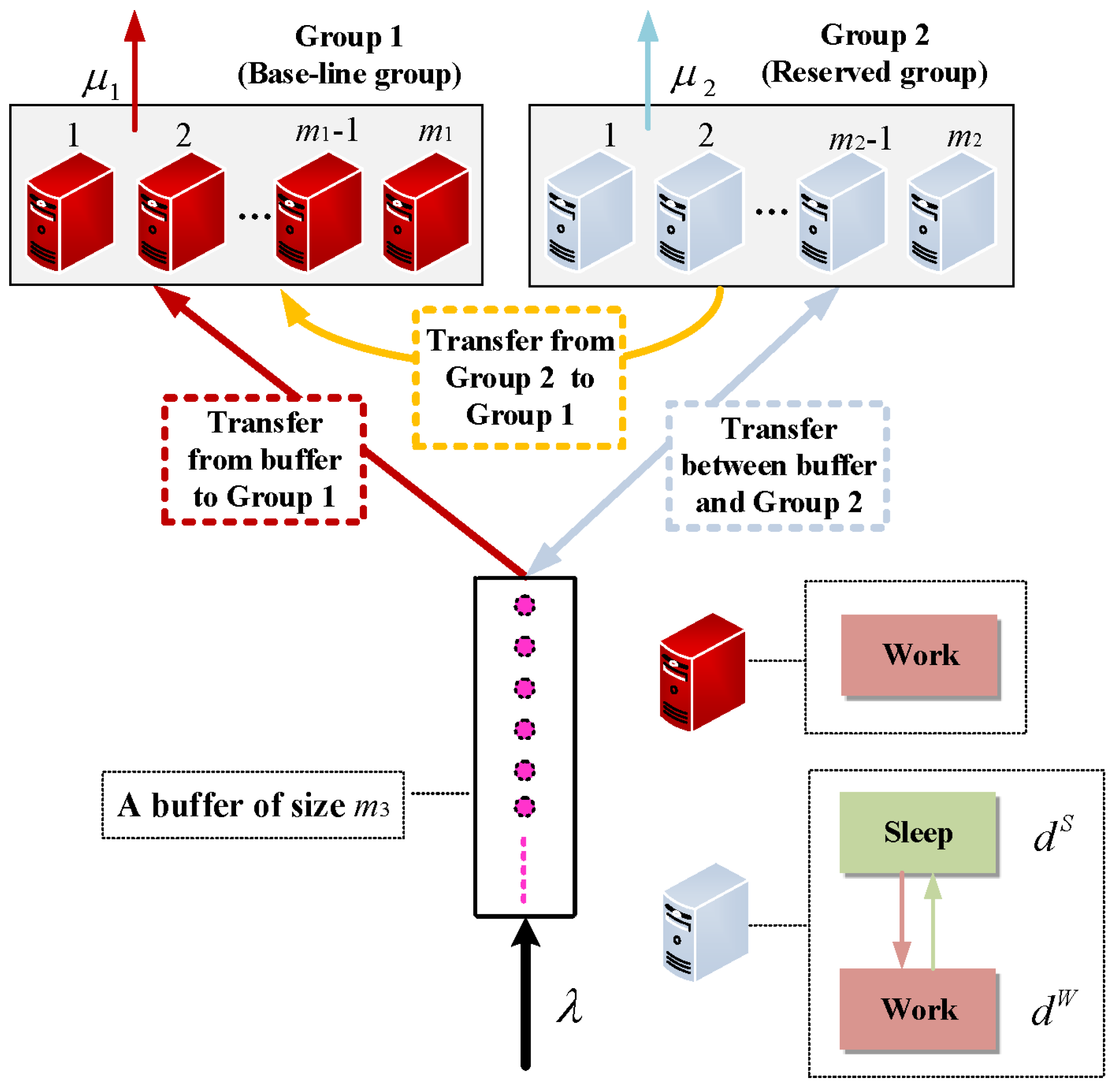
:In this paper, we apply a Markov decision process to find the optimal asynchronous dynamic policy of an energy-efficient data center with two server groups. Servers in Group 1 always work, while servers in Group 2 may either work or sleep, and a fast setup process occurs when the server’s states are changed from sleep to work. The servers in Group 1 are faster and cheaper than those of Group 2 so that Group 1 has a higher service priority. Putting each server in Group 2 to sleep can reduce system costs and energy consumption, but it must bear setup costs and transfer costs. For such a data center, an asynchronous dynamic policy is designed as two sub-policies: The setup policy and the sleep policy, both of which determine the switch rule between the work and sleep states for each server in Group 2. To find the optimal asynchronous dynamic policy, we apply the sensitivity-based optimization to establish a block-structured policy-based Markov process and use a block-structured policy-based Poisson equation to compute the unique solution of the performance potential by means of the RG-factorization. Based on this, we can characterize the monotonicity and optimality of the long-run average profit of the data center with respect to the asynchronous dynamic policy under different service prices. Furthermore, we prove that a bang–bang control is always optimal for this optimization problem. We hope that the methodology and results developed in this paper can shed light on the study of more general energy-efficient data centers.
1. Introduction
Over the last two decades considerable attention has been given to studying energy- efficient data centers. On the one hand, as the number and size of data centers increase rapidly, energy consumption becomes one main part of the operating costs of data centers. On the other hand, data centers have become a fundamental part of the IT infrastructure in today’s Internet services, in which a huge number of servers are deployed in each data center such that the data centers can provide cloud computing environments. Therefore, finding optimal energy-efficient policies and designing optimal energy-efficient mechanisms are always interesting, difficult, and challenging in the energy-efficient management of data centers. Readers may refer to recent excellent survey papers, such as Masanet et al. [1], Zhang et al. [2], Nadjahi et al. [3], Koot and Wijnhoven [4], Shirmarz and Ghaffari [5], Li et al. [6], and Harchol-Balter [7].
Barroso and Hölzle [8] demonstrated that many data centers were designed to handle peak loads effectively, but this directly caused a significant number of servers (approximately 20%) in the data centers to be idle because no work was done in the off-peak period. Although the idle servers do not provide any services, they still continue to consume a notable amount of energy, which is approximately 70% of the servers working in the on-peak period. Therefore, it is necessary and useful to design an energy-efficient mechanism for specifically dealing with idle servers. In this case, a key technique, the energy-efficient states of “Sleep” or “Off” were introduced such that the idle servers can take the sleep or off state, which always consumes less energy, in which the sleep state consumes very little energy, while the energy consumption of the off state is zero. See Kuehn and Mashaly [9] for more interpretation. To analyze the energy-efficient states, thus far, some queueing systems either with server energy-efficient states (e.g., work, idle, sleep, and off) or with server control policies (e.g., vacation, setup, and N-policy) have been developed in the study of energy-efficient data centers. Important examples include the survey papers by Gandhi [10] and Li et al. [6], and the research papers by Gandhi et al. [11,12,13], Maccio and Down [14,15], Phung-Duc [16] and Phung-Duc and Kawanishi [17].
It is always necessary to design an optimal energy-efficient mechanism for data centers. To do this, several static optimization methods have been developed using two basic approaches. The first is to construct a suitable utility function for a performance-energy trade-off or a performance cost with respect to the synchronous optimization of different performance measures, for example, reducing energy consumption, reducing system response time, and improving quality of service. The second is to minimize the performance cost by means of some optimal methods, including linear programming, nonlinear programming, and integer programming. Gandhi et al. [12] provided two classes of the performance-energy trade-offs: (a) ERWS, the weighted sum of the mean response time and the mean power cost , where are weighted coefficients; (b) ERP, the product of the mean response time and the mean power cost. See Gandhi et al. [12] and Gandhi [10] for systematical research. Maccio and Down [14] generalized the ERP to a more general performance cost function that considers the expected cycle rate. Gebrehiwot et al. [18] made some interesting generalizations of the ERP and ERWS by introducing multiple intermediate sleep states. Additionally, Gebrehiwot et al. [19,20] generalized the FCFS queue of the data center with multiple intermediate sleep states to the processor-sharing discipline and to the shortest remaining processing time (SRPT) discipline, respectively. In addition, Mitrani [21,22] provided another interesting method to discuss the data center of N identical servers that contain m reserves, while the idle or work of the servers is controlled by an up threshold U and a down threshold D. He established a new performance cost and provided expressions for the average numbers and , so that the performance cost C can be optimized with respect to the three key parameters m, U, and D.
To date, little work has been done on applications of Markov decision processes (MDPs) to find the optimal dynamic control policies of energy-efficient data centers. Readers may refer to recent publications for details, among which Kamitsos et al. [23] constructed a discrete-time MDP and proved that the optimal sleep energy-efficient policy is simply hysteretic, so that it has a double threshold structure. Note that such an optimal hysteretic policy follows Hipp and Holzbaur [24] and Lu and Serfozo [25]. For policy optimization and dynamic power management for electronic systems or equipment, the MDPs and stochastic network optimization were developed from five different perspectives: (a) the discrete-time MDPs by Yang et al. [26]; (b) the continuous-time MDPs by Ding et al. [27]; (c) stochastic network optimization by Liang et al. [28]; (d) the sensitivity-based optimization by Xia and Chen [29], Xia et al. [30], and Ma et al. [31]; and (e) the deep reinforcement learning by Chi et al. [32].
The purpose of this paper is to apply continuous-time MDPs to set up optimal dynamic energy-efficient policies for data centers, in which the sensitivity-based optimization is developed to find the optimal solution. Note that the sensitivity-based optimization is greatly refined from the MDPs by dealing with the Poisson equation by means of some novel tools, for instance, performance potential and performance difference. To date, the sensitivity-based optimization has also been sufficiently related to the Markov reward processes (see Li [33]), thus, it is an effective method for the performance optimization of many practical systems (see an excellent book by Cao [34] for more details). The sensitivity-based optimization theory has been applied to performance optimization in many practical areas. For example, in energy-efficient data centers by Xia et al. [35]; inventory rationing by Li et al. [36]; the blockchain selfish mining by Ma and Li [37]; and in finance by Xia [38].
The main contributions of this paper are threefold. The first contribution is to apply the sensitivity-based optimization (and the MDPs) to study a more general energy-efficient data center with key practical factors, for example, a finite buffer, a fast setup process, and transferring some incomplete service jobs to the idle servers in Group 1 or to the finite buffer, if any. Although practical factors will not increase any difficulty in performance evaluation (e.g., modeling by means of queueing systems or Markov processes, also see Gandhi [10] for more details), they can largely cause substantial difficulties and challenges in finding optimal dynamic energy-efficient policies and, furthermore, in determining threshold-type policies by using the sensitivity-based optimization. For instance, the finite buffer makes the policy-based Markov process appear as the two-dimensional block-structured Markov process from the one-dimensional birth–death process given in Ma et al. [31] and Xia et al. [35].
Note that this paper has two related works: Ma et al. [31] and Xia et al. [35], and it might be necessary to set up some useful relations between this paper and each of the two papers. Compared with Ma et al. [31], this paper considers more practical factors in the energy-efficient data centers such that the policy-based Markov process is block-structured, which makes solving the block-structured Poisson equation more complicated. Compared with Xia et al. [35], this paper introduces a more detailed cost and reward structure, which makes an analysis of the monotonicity and optimality of dynamic energy-efficient policies more difficult and challenging. Therefore, this paper is a necessary and valuable generalization of Ma et al. [31] and Xia et al. [35] through extensively establishing the block-structured policy-based Markov processes, which in fact are the core part of the sensitivity-based optimization theory and its applications in various practical systems.
The second contribution of this paper is that it is the first to find an optimal asynchronous dynamic policy in the study of energy-efficient data centers. Note that the two groups of servers in the data center have “the setup actions from the sleep state to the work state” and “the close actions from the work state to the sleep state”, thus, we follow the two action steps to form an asynchronous dynamic policy, which is decomposed into two sub-policies: the setup policy (or the setup action) and the sleep policy (or the close action). Crucially, one of the successes of this paper is to find the optimal asynchronous dynamic policy from many asynchronous dynamic policies by means of the sensitivity-based optimization. To date, it has still been very difficult and challenging in the MDPs.
The third contribution of this paper is to provide a unified framework for applying the sensitivity-based optimization to study the optimal asynchronous dynamic policy of the energy-efficient data center. For such a more complicated energy-efficient data center, we first establish a policy-based block-structured Markov process as well as a more detailed cost and reward structure, and provide an expression for the unique solution to the block-structured Poisson equation by means of the RG-factorization. Then, we show the monotonicity of the long-run average profit with respect to the setup and sleep policies and the asynchronous policy, respectively. Based on this, we find the optimal asynchronous policy when the service price is higher (or lower) than a key threshold. Finally, we indicate that the optimal control is a bang–bang control. Such a structure of the optimal asynchronous energy-efficient policy reduces the search space, which is a significant reduction of the optimization complexity and effectively alleviates the curse of the dimensionality of MDPs. Therefore, the optimal asynchronous dynamic policy is the threshold-type in the energy-efficient data center. Note that the optimality of the threshold-type policy can realize a large reduction for the search space, thus, the optimal threshold-type policy is of great significance to solve the mechanism design problem of energy-efficient data centers. Therefore, the methodology and results developed in this paper provide new highlights for understanding dynamic energy-efficient policy optimization and mechanism design in the study of more general data centers.
The organization of this paper is as follows. In Section 2, we give a problem description for an energy-efficient data center with more practical factors. In Section 3, we establish a policy-based continuous-time block-structured Markov process and define a suitable reward function with respect to both states and policies of the Markov process. In Section 4, we set up a block-structured Poisson equation and provide an expression for its unique solution by means of the RG-factorization. In Section 5, we study a perturbation realization factor of the policy-based continuous-time block-structured Markov process for the asynchronous dynamic policy, and analyze how the service price impacts on the perturbation realization factor. In Section 6, we discuss the monotonicity and optimality of the long-run average profit of the energy-efficient data center with respect to the asynchronous policy. Based on this, we can give the optimal asynchronous dynamic policy of the energy-efficient data center. In Section 7, if the optimal asynchronous dynamic policy is the threshold-type, then we can compute the maximal long-run average profit of the energy-efficient data center. In Section 8, we give some concluding remarks. Finally, three appendices are given, both for the state-transition relation figure of the policy-based block-structured continuous-time Markov process and for the block entries of its infinitesimal generator.
2. Model Description
In this section, we provide a problem description for setting up and optimizing an asynchronous dynamic policy in an energy-efficient data center with two groups of different servers, a finite buffer, and a fast setup process. Additionally, we provide the system structure, operational mode, and mathematical notations in the energy-efficient data center.
Server groups: The data center contains two server groups: Groups 1 and 2, each of which is also one interactive subsystem of the data center. Groups 1 and 2 have and servers, respectively. Servers in the same group are homogeneous, while those in different groups are heterogeneous. Note that Group 1 is viewed as a base-line group whose servers are always at the work state even if some of them are idle, the purpose of which is to guarantee a necessary service capacity in the data center. Hence, each server in Group 1 always works regardless of whether it has a job or not, so that it must consume an amount of energy at any time. In contrast, Group 2 is regarded as a reserved group whose servers may either work or sleep so that each of the servers can switch its state between work and sleep. If one server in Group 2 is at the sleep state, then it consumes a smaller amount of energy than the work state, as maintaining only the sleep state requires very little energy.
A finite buffer: The data center has a finite buffer of size . Jobs must first enter the buffer, and then they are assigned to the groups (Group 1 is prior to Group 2) and subsequently to the servers. To guarantee that the float service capacity of Group 2 can be fully utilized when some jobs are taken from the buffer to Group 2, we assume that , i.e., the capacity of the buffer must be no less than the server number of Group 2. Otherwise, if there are more jobs waiting in the buffer, the jobs transferred from Group 2 to the buffer will be lost.
Arrival processes: The arrivals of jobs at the data center are a Poisson process with arrival rate . If the buffer is full, then any arriving job has to be lost immediately. This leads to an opportunity cost per unit of time for each lost job due to the full buffer.
Service processes: The service times provided by each server in Groups 1 and 2 are i.i.d. and exponential with service rates and , respectively. We assume that which makes the prior use of servers in Group 1. The service discipline of each server in the data center is First Come First Serve (FCFS). If a job finishes its service at a server, then it immediately leaves the system. At the same time, the data center can obtain a fixed service reward (or service price) from the served job.
Once a job enters the data center for its service, it has to pay holding costs per unit of time , and in Group 1, Group 2, and the buffer, respectively. We assume that also guarantees the prior use of servers in Group 1. Therefore, to support the service priority, each server in Group 1 is not only faster but also cheaper than that in Group 2.
Switching between work and sleep: To save energy, the servers in Group 2 can switch between the work and sleep states. On the one hand, if there are more jobs waiting in the buffer, then Group 2 sets up and turns on some sleeping servers. This process usually involves a setup cost However, the setup time is very short as it directly begins from the sleep state and it can be ignored. On the other hand, if the number of jobs in Group 2 is smaller, then the working servers are switched to the sleep state, while the incomplete-service jobs are transferred to the buffer and served as the arriving ones.
Transfer rules: (1) To Group 1. Based on the prior use of servers in Group 1, if a server in Group 1 becomes idle and there is no job in the buffer, then an incomplete-service job (if it exists) in Group 2 must immediately be transferred to the idle server in Group 1. Additionally, the data center needs to pay a transferred cost to the transferred job.
(2) To the buffer. If some servers in Group 2 are closed to the sleep state, then those jobs in the servers closed at the sleep state are transferred to the buffer, and a transferred cost is paid by the data center.
To keep the transferred jobs that can enter the buffer, we need to control the new jobs arriving at the buffer. If the sum of the job number in the buffer and the job number in Group 2 is equal to , then the newly arriving jobs must be lost immediately.
Power Consumption: The power consumption rates and are for the work states of servers in Groups 1 and 2, respectively, while is only for the sleep state of a server in Group 2. Note that each server in Group 1 does not have the sleep state and it is clear that . We assume that . There is no power consumption for keeping the jobs in the buffer. is the power consumption price per unit of the power consumption rate and per unit of time.
Independence: We assume that all the random variables in the data center defined above are independent.
Finally, to aid reader understanding, the data center, together with its operational mode and mathematical notations, is depicted in Figure 1. Table 1 summarizes some notations involved in the model. This will be helpful in our later study.
In the remainder of this section, it might be useful to provide some comparison of the above model assumptions with those in Ma et al. [31] and in Xia et al. [35].
Remark 1.
(1) Compared with our previous paper [31], this paper considers several new practical factors, such as a finite buffer, a fast setup process, and a job transfer rule. The new factors make our MDP modeling more practical and useful in the study of energy-efficient data centers. Although the new factors do not increase any difficulty in performance evaluation through modeling by means of queueing systems or Markov processes, they can cause substantially more difficulties and challenges in finding optimal dynamic energy-efficient policies and, furthermore, in determining threshold-type policies by using the sensitivity-based optimization. Note that the difficulties mainly grow out of establishing the policy-based block-structured Markov process and solving the block-structured Poisson equation. On this occasion, we have simplified the above model descriptions: for example, the setup is immediate, the jobs can be transferred without delay either between the slow and fast servers or between the slow servers and the buffer, the jobs must be transferred as soon as the fast server becomes free, the finite buffer space is reserved for jobs in progress, and so on.
(2) For the energy-efficient data center operating with some buffer, it is seen from Figure A3 in Appendix B that the main challenge of our work is to focus on how to describe the policy-based block-structured Markov process. Obviously, (a) if there are more than two groups of servers, then it is easy to check that the policy-based Markov process will become multi-dimensional so that its analysis is very difficult; (b) if the buffer is infinite, then we have to deal with the policy-based block-structured Markov process with infinitely many levels, for which the discussion and computation are very complicated.
Remark 2.
Compared with Xia et al. [35], this paper introduces a more detailed cost and reward structure, which makes analysis for the monotonicity and optimality of the dynamic energy-efficient policies more difficult and challenging. Therefore, many cost and reward factors make the MDP analysis and the sensitivity-based optimization more complicated.
3. Optimization Model Formulation
In this section, for the energy-efficient data center, we first establish a policy-based continuous-time Markov process with a finite block structure. Then, we define a suitable reward function with respect to both states and policies of the Markov process. Note that this will be helpful and useful for setting up a MDP to find the optimal asynchronous dynamic policy in the energy-efficient data center.
3.1. A Policy-Based Block-Structured Continuous-Time Markov Process
The data center in Figure 1 shows Group 1 of servers, Group 2 of servers, and a buffer of size . We need to introduce both “states” and “policies” to express the stochastic dynamics of this data center. Let , and be the numbers of jobs in Group 1, Group 2, and the buffer, respectively. Therefore, is regarded as a state of the data center at time t. Let all the cases of such a state form a set as follows:
where
For a state it is seen from the model description that there are four different cases: (a) By using the transfer rules, if , then if either or , then . (b) If and then the jobs in the buffer can increase until the waiting room is full, i.e., (c) If and then the total numbers of jobs in Group 2 and the buffer are no more than the buffer size, i.e., (d) If and then the jobs in the buffer can also increase until the waiting room is full, i.e.,
Now, for Group 2, we introduce an asynchronous dynamic policy, which is related to two dynamic actions (or sub-policies): from sleep to work (setup) and from work to sleep (close). Let and be the numbers of working servers and of sleeping servers in Group 2 at State , respectively. By observing the state set , we call and the setup policy (i.e., from sleep to work) and the sleep policy (i.e., from work to sleep), respectively.
Note that the servers in Group 2 can only be set up when all of them are idle, while we cannot simultaneously have the setup policy () because the servers in Group 2 are always affected by the sleep policy () if they still work for some jobs. This is what we call asynchronous dynamic policies. Here, we consider the control optimization of the total system. For such sub-policies, we provide an interpretation of four different cases as follows:
(1) In if , then due to the transfer rule. Thus, there are no jobs in Group 2 or in the buffer, so that no policy in Group 2 is used;
(2) In the states will affect how to use the setup policy. If , , then is the number of working servers in Group 2 at State . Note that some of the slow servers need to first start, so that some jobs in the buffer can enter the activated slow servers, thus, , each of which can possibly take place under an optimal dynamic policy;
(3) From to the states will affect how to use the sleep policy. If , , then is the number of sleeping servers in Group 2 at State We assume that the number of sleeping servers is no less than . Note that the sleep policy is independent of the work policy. Once the sleep policy is set up, the servers without jobs must enter the sleep state. At the same time, some working servers with jobs are also closed to the sleep state, and the jobs in those working servers are transferred to the buffer. It is easy to see that
(4) In if and , then may be any element in the set it is clear that
Our aim is to determine when or under what conditions an optimal number of servers in Group 2 switch between the sleep state and the work state such that the long-run average profit of the data center is maximal. From the state space , we define an asynchronous dynamic energy-efficient policy as
where and are the setup and sleep policies, respectively; ‘⊠’ denotes that the policies and occur asynchronously; and
Note that is related to the fact that if there is no job in Group 2 at the initial time, then all the servers in Group 2 are at the sleep state. Once there are jobs in the buffer, we quickly set up some servers in Group 2 such that they enter the work state to serve the jobs. Similarly, we can understand the sleep policy In the state subset it is seen that the setup policy will not be needed because some servers are kept at the work state.
For all the possible policies given in (1), we compose a policy space as follows:
Let for any given policy . Then is a policy-based block-structured continuous-time Markov process on the state space whose state transition relations are given in Figure A3 in Appendix B (we provide two simple special cases to understand such a policy-based block-structured continuous-time Markov process in Appendix A). Based on this, the infinitesimal generator of the Markov process is given by
where every block element depends on the policy (for simplification of description, here we omit “”) and it is expressed in Appendix C.
It is easy to see that the infinitesimal generator has finite states, and it is irreducible with , thus, the Markov process is a positive recurrent. In this case, we write the stationary probability vector of the Markov process as
where
Note that the stationary probability vector can be obtained by means of solving the system of linear equations and where is a column vector of the ones with a suitable size. To this end, the RG-factorizations play an important role in our later computation. Note that some computational details are given in Chapter 2 in Li [33].
Now, we use UL-type RG-factorization to compute the stationary probability vector as follows. For and , we write
Clearly, and . Let
and
Then the UL-type RG-factorization is given by
where
and
By using Theorem 2.9 of Chapter 2 in Li [33], the stationary probability vector of the Markov process is given by
where is the stationary probability vector of the censored Markov chain to level 0, and the positive scalar is uniquely determined by
Remark 3.
The RG-factorizations provide a unified, constructive and algorithmic framework for the numerical computation of many practical stochastic systems. It can be applied to provide effective solutions for the block-structured Markov processes, and are shown to be also useful for the optimal design and dynamical decision-making of many practical systems. See more details in Li [33].
The following theorem provides some useful observations on some special policies , in which the special policies will have no effect on the infinitesimal generator or the stationary probability vector .
Theorem 1.
Suppose that two asynchronous energy-efficient policies satisfy one of the following two conditions: for each , if , then we take as any element of the set ; for each if , then we take Under both such conditions, we have
Proof of Theorem 1.
It is easy to see from (2) that all the levels of the matrix are the same as those of the matrix , except level 1. Thus, we only need to compare level 1 of the matrix with that of the matrix .
For the two asynchronous energy-efficient policies satisfying the conditions (a) and (b), by using in (2), it is clear that for , if , then
Thus, it follows from (2) that This also gives that and thus This completes the proof. □
Note that Theorem 1 will be necessary and useful for analyzing the policy monotonicity and optimality in our later study. Furthermore, see the proof of Theorem 4.
Remark 4.
This paper is the first to introduce and consider the asynchronous dynamic policy in the study of energy-efficient data centers. We highlight the impact of the two asynchronous sub-policies: the setup and sleep policies on the long-run average profit of the energy-efficient data center.
3.2. The Reward Function
For the Markov process , now we define a suitable reward function for the energy-efficient data center.
Based on the above costs and price notations in Table 1, a reward function with respect to both states and policies is defined as a profit rate (i.e., the total revenues minus the total costs per unit of time). Therefore, according to the impact of the asynchronous dynamic policy on the profit rate, the reward function at State under policy is divided into four cases as follows:
Case (a): For and , the profit rate is not affected by any policy, and we have
Note that in Case (a), there is no job in Group 2 or in the buffer. Thus, it is clear that each server in Group 2 is at the sleep state.
However, in the following two cases (b) and (c), since there are some jobs either in Group 2 or in the buffer, the policy will play a key role in opening (i.e., setup) or closing (i.e., sleep) some servers of Group 2 to save energy efficiently.
Case (b): For , and the profit rate is affected by the setup policy , we have
where is an indicator function whose value is 1 when the event is in , otherwise its value is 0.
Case (c): For , and , the profit rate is affected by the sleep policy , we have
Note that the job transfer rate from Group 2 to Group 1 is given by . If , then and . If and , then . If and , then .
Case (d): For , and , the profit rate is not affected by any policy, we have
We define a column vector composed of the elements , and as
where
In the remainder of this section, the long-run average profit of the data center (or the policy-based continuous-time Markov process ) under an asynchronous dynamic policy is defined as
where and are given by (3) and (8), respectively.
We observe that as the number of working servers in Group 2 decreases, the total revenues and the total costs in the data center will decrease synchronously, and vice versa. On the other hand, as the number of sleeping servers in Group 2 increases, the total revenues and the total costs in the data center will decrease synchronously, and vice versa. Thus, there is a tradeoff between the total revenues and the total costs for a suitable number of working and/or sleeping servers in Group 2 by using the setup and sleep policies, respectively. This motivates us to study an optimal dynamic control mechanism for the energy-efficient data center. Thus, our objective is to find an optimal asynchronous dynamic policy such that the long-run average profit is maximized, that is,
Since the setup and sleep policies and occur asynchronously, they cannot interact with each other at any time. Therefore, it is seen that the optimal policy can be decomposed into
In fact, it is difficult and challenging to analyze the properties of the optimal asynchronous dynamic policy , and to provide an effective algorithm for computing the optimal policy . To do this, in the next sections we will introduce the sensitivity-based optimization theory to study this energy-efficient optimization problem.
4. The Block-Structured Poisson Equation
In this section, for the energy-efficient data center, we set up a block-structured Poisson equation which provides a useful relation between the sensitivity-based optimization and the MDP. Additionally, we use the RG-factorization, given in Li [33], to solve the block-structured Poisson equation and provide an expression for its unique solution.
For , it follows from Chapter 2 in Cao [34] that for the policy-based continuous-time Markov process , we define the performance potential as
where is defined in (9). It is seen from Cao [34] that for any policy , quantifies the contribution of the initial state to the long-run average profit of the data center. Here, is also called the relative value function or the bias in the traditional Markov decision process theory, see, e.g., Puterman [39] for more details. We further define a column vector with elements for
where
A similar computation to that in Ma et al. [31], the block-structured Poisson equation is given by
where is defined in (9), is given in (8), and is given in (2).
To solve the system of linear equations (13), we note that rank and because the size of the matrix is . Hence, this system (13) of linear equations exists with infinitely many solutions with a free constant of an additive term. Let be a matrix obtained through omitting the first row and the first column vectors of the matrix . Then,
where
is obtained by means of omitting the first row vector of , and are obtained from omitting the first column vectors of and , respectively. The other block entries in are the same as the corresponding block entries in the matrix
Note that, rank and the size of the matrix is . Hence, the matrix is invertible.
Let and be two column vectors of size obtained through omitting the first element of the two column vectors and of size , respectively, and
Then,
where and are the two column vectors, which are obtained through omitting the scale entries and of and respectively, and
Therefore, it follows from (13) that
where is a column vector with the first element being one and all the others being zero. Note that the matrix is invertible and , thus the system (16) of linear equations always exists with one unique solution:
where is any given positive constant. For the convenience of computation, we take . In this case, we have
Note that the expression of the invertible matrix can be obtained by means of the RG-factorization, which is given in Li [33] for general Markov processes.
For convenience of computation, we write
and every element of the matrix is written by a scalar , we denote by n a system state under the certain block, and l the index of element, where , , for and
It is easy to check that
for
and
The following theorem provides an expression for the vector under a constraint condition . Note that this expression is very useful for applications of the sensitivity-based optimization theory to the study of Markov decision processes in our later study.
Theorem 2.
If , then for
for
for and
for
Proof of Theorem 2.
It is seen from (18) that we need to compute two parts: and . Note that
thus a simple computation for the vector can obtain our desired results. This completes the proof. □
5. Impact of the Service Price
In this section, we study the perturbation realization factor of the policy-based continuous-time Markov process both for the setup policy and for the sleep policy (i.e., they form the asynchronous energy-efficient policy), and analyze how the service price impacts on the perturbation realization factor. To do this, our analysis includes the following two cases: the setup policy and the sleep policy. Note that the results given in this section will be useful for establishing the optimal asynchronous dynamic policy of the energy-efficient data center in later sections.
It is a key in our present analysis that the setup policy and the sleep policy are asynchronous at any time; thus, we can discuss the perturbation realization factor under the asynchronous dynamic policy from two different computational steps.
5.1. The Setup Policy
For the performance potential vector under a constraint condition , we define a perturbation realization factor as
where We can see that quantifies the difference between two performance potentials and . It measures the long-run effect on the average profit of the data center when the system state is changed from to . For our next discussion, through observing the state space, it is necessary to define some perturbation realization factors as follows:
where and
It follows from Theorem 2 that
To express the perturbation realization factor by means of the service price R, we write
for and ,
for , and ,
for , and , ,,
for , and , ,,
Then for and , ,
for , and ,
for , and , ,,
for , and , ,,
We rewrite as
Then it is easy to check that
and
Thus, we obtain
If a job finishes its service at a server and leaves this system immediately, then the data center can obtain a fixed revenue (i.e., the service price) R from such a served job. Now, we study the influence of the service price R on the perturbation realization factor. Note that all the numbers are positive and are independent of the service price R, while all the numbers are the linear functions of R. We write
and
then for , we obtain
Now, we define
where is defined as
From the later discussion in Section 6, we will see that plays a fundamental role in the performance optimization of data centers, and the sign of directly determines the selection of decision actions, as shown in (38) later. To this end, we analyze how the service price can impact on as follows. Substituting (21) into the linear equation , we obtain
where and
It is easy to see from (22) that (a) if , then ; and (b) if , then .
In the energy-efficient data center, we define two critical values, related to the service price, as
and
The following proposition uses the two critical values, which are related to the service price, to provide a key condition whose purpose is to establish a sensitivity-based optimization framework of the energy-efficient data center in our later study. Additionally, this proposition will be useful in the next section for studying the monotonicity of the asynchronous energy-efficient policies.
Proposition 1.
(1) If , then for any and for each couple with we have
(2) If , then for any and for each couple with we have
Proof of Proposition 1.
(1) For any and for each couple with , since and , this gives
Thus, for any couple with this makes that .
(2) For any and for each couple with , if , we get
this gives that . This completes the proof. □
5.2. The Sleep Policy
The analysis for the sleep policy is similar to that of the setup policy given in the above subsection. Here, we shall provide only a simple discussion.
We define the perturbation realization factor for the sleep policy as follows:
where and
It follows from Theorem 2 that
Similarly, to express the perturbation realization factor by means of the service price R, we write
where
and
Now, we analyze how the service price impacts on as follows: Substituting (29) into the linear equation , we obtain
It is easy to see from Equation (30) that (a) if , then ; and (b) if , then .
In the energy-efficient data center, we relate to the service price and define two critical values as
and
The following proposition is similar to Proposition 1, thus its proof is omitted here.
Proposition 2.
(1) If , then for any and for each couple with we have
(2) If , then for any and for each couple with we have
From Propositions 1 and 2, we relate to the service price and define two new critical values as
The following theorem provides a simple summarization from Propositions 1 and 2, and it will be useful for studying the monotonicity and optimality of the asynchronous dynamic policy in our later sections.
Theorem 3.
(1) If , then for any asynchronous dynamic policy , we have
(2) If , then for any asynchronous policy , we have
6. Monotonicity and Optimality
In this section, we use the block-structured Poisson equation to derive a useful performance difference equation, and discuss the monotonicity and optimality of the long-run average profit of the energy-efficient data center with respect to the setup and sleep policies, respectively. Based on this, we can give the optimal asynchronous dynamic policy of the energy-efficient data center.
The standard Markov model-based formulation suffers from a number of drawbacks. First and foremost, the state space is usually too large for practical problems. That is, the number of potentials to be calculated or estimated is too large for most problems. Secondly, the generally applicable Markov model does not reflect any special structure of a particular problem. Thus, it is not clear whether and how potentials can be aggregated to save computation by exploring the special structure of the system. The sensitivity point of view and the flexible construction of the sensitivity formulas provide us a new perspective to explore alternative approaches for the performance optimization of systems with some special features.
For any given asynchronous energy-efficient policy , the policy-based continuous-time Markov process with infinitesimal generator given in (2) is an irreducible, aperiodic, and positive recurrent. Therefore, by using a similar analysis to Ma et al. [31], the long-run average profit of the data center is given by
and the Poisson equation is written as
For State , it is seen from (2) that the asynchronous energy-efficient policy directly affects not only the elements of the infinitesimal generator but also the reward function . That is, if the asynchronous policy changes, then the infinitesimal generator and the reward function will have their corresponding changes. To express such a change mathematically, we take two different asynchronous energy-efficient policies and , both of which correspond to their infinitesimal generators and , and to their reward functions and .
The following lemma provides a useful equation for the difference of the long-run average performances and for any two asynchronous policies . Here, we only restate it without proof, while readers may refer to Ma et al. [31] for more details.
Lemma 1.
For any two asynchronous energy-efficient policies , we have
Now, we describe the first role played by the performance difference, in which we set up a partial order relation in the policy set so that the optimal asynchronous energy-efficient policy in the finite set can be found by means of finite comparisons. Based on the performance difference for any two asynchronous energy-efficient policies , we can set up a partial order in the policy set as follows. We write if ; if ; if . Furthermore, we write if ; if . By using this partial order, our research target is to find an optimal asynchronous policy such that for any asynchronous energy-efficient policy , or
Note that the policy set and the state space are both finite, thus an enumeration method is feasible for finding the optimal asynchronous energy-efficient policy in the policy set . Since
It is seen that the policy set contains elements so that the enumeration method used to find the optimal policy will require a huge enumeration workload. However, our following work will be able to greatly reduce the amount of searching for the optimal asynchronous policy by means of the sensitivity-based optimization theory.
Now, we discuss the monotonicity of the long-run average profit with respect to any asynchronous policy under the different service prices. Since the setup and sleep policies and occur asynchronously and they will not interact with each other at any time, we can, respectively, study the impact of the policies and on the long-run average profit To this end, in what follows we shall discuss three different cases: , and
6.1. The Service Price
In the case of we discuss the monotonicity and optimality with respect to two different policies: the setup policy and the sleep policy, respectively.
6.1.1. The Setup Policy with
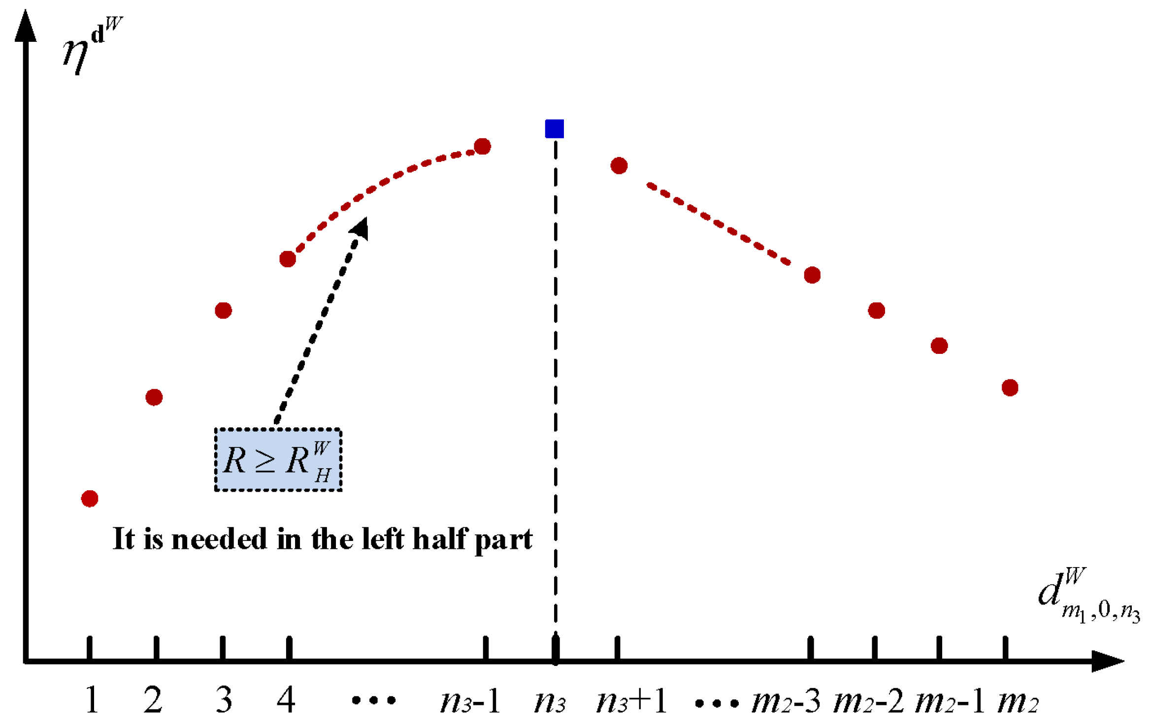
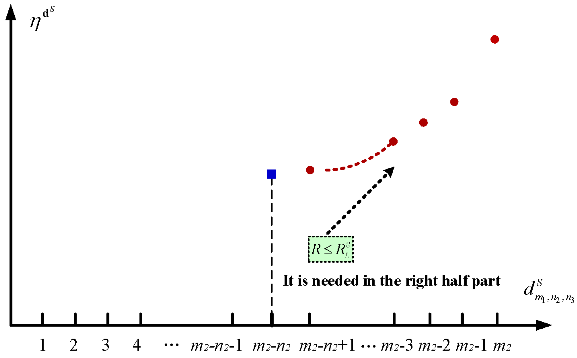
The following theorem analyzes the right-half part of the unimodal structure (see Figure 2) of the long-run average profit with respect to the setup policy—either if or if .
Theorem 4.
For any setup policy with and for each , the long-run average profit is linearly increasing with respect to the setup policy either if or if .
Proof of Theorem 4.
For each , we consider two interrelated policies as follows:
where . It is seen that the two policies have one difference only between their corresponding decision elements and . In this case, it is seen from Theorem 1 that and . Furthermore, it is easy to check from (4) to (7) that
Thus, it follows from Lemma 1 that
or
Since , it is easy to see that can be determined by This indicates that is irrelevant to the decision element Furthermore, note that is irrelevant to the decision element , and , and are all positive constants, thus it is easy to see from (35) that the long-run average profit is linearly decreasing with respect to each decision element for . It is worth noting that if then . This completes the proof. □
In what follows, we discuss the left-half part of the unimodal structure (see Figure 2) of the long-run average profit with respect to each decision element if Compared to analysis of its right-half part, our discussion for the left-half part is a little bit complicated.
Let the optimal setup policy be
Then, it is seen from Theorem 4 that
Hence, Theorem 4 takes the area of finding the optimal setup policy from a large set to a greatly shrunken area .
To find the optimal setup policy , we consider two setup policies with an interrelated structure as follows:
where , and . It is easy to check from (2) that
Hence, we have
We write that
The following theorem discusses the left-half part (see Figure 2) of the unimodal structure of the long-run average profit with respect to each decision element .
Theorem 5.
If , then for any setup policy with and for each , the long-run average profit is strictly monotone and increasing with respect to each decision element for
Proof of Theorem 5.
For each , we consider two setup policies with an interrelated structure as follows:
where , and . Applying Lemma 1, it follows from (36)and (37) that
If , then it is seen from Proposition 1 that . Thus, we get that for the two policies with and ,
This shows that
This completes the proof. □
When , now we use Figure 2 to provide an intuitive summary for the main results given in Theorems 4 and 5. In the right-half part of Figure 2,
shows that is a linear function of the decision element . By contrast, in the right-half part of Figure 2, we need to first introduce a restrictive condition: , under which
Since also depends on the decision element , it is clear that is a nonlinear function of the decision element .
6.1.2. The Sleep Policy with
It is different from the setup policy in that, for the sleep policy, each decision element is . Hence, we just consider the structural properties of the long-run average profit with respect to each decision element .
We write the optimal sleep policy as where
Then, it is seen that
It is easy to see that the area of finding the optimal sleep policy is .
To find the optimal sleep policy , we consider two sleep policies with an interrelated structure as follows:
where , , it is easy to check from (2) that
On the other hand, from the reward functions given in (6), is in either for and or for and we have
and
Hence, we have
We write
The following theorem discusses the structure of the long-run average profit with respect to each decision element .
Theorem 6.
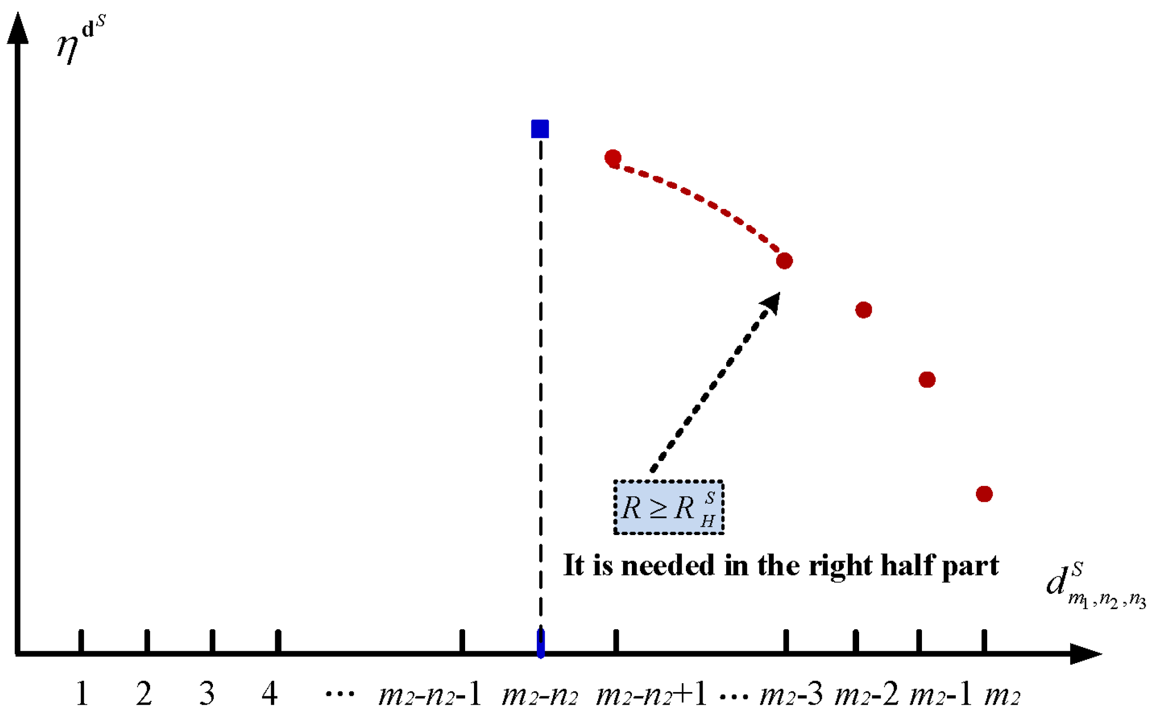
If , then for any sleep policy with and for each , , the long-run average profit is strictly monotone decreasing with respect to each decision element .
Proof of Theorem 6.
For each and , we consider two sleep policies with an interrelated structure as follows:
where , and . Applying Lemma 1, it follows from (39)and (40) that
It is worthwhile to note that (41) has the same form as (38), since the perturbation of the sleep policy, , and denote the number of the working servers. If , then it is seen from Proposition 1 that for we have . Thus, we get that for and ,
this shows that is strictly monotone increasing with respect to . Thus, we get that for the two policies with and ,
It is easy to see that
This completes the proof. □
When , now we use Figure 3 to provide an intuitive summary for the main results given in Theorems 6. According to (41), depends on , and it is clear that is a nonlinear function of .
As a simple summarization of Theorems 5 and 6, we obtain the monotone structure of the long-run average profit with respect to the asynchronous energy-efficient policy, while its proof is easy only on the condition that makes and .
Theorem 7.
If , then for any policy , the long-run average profit is strictly monotone with respect to each decision element of and of , respectively.
6.2. The Service Price
A similar analysis to that of the case we simply discuss the service price for the monotonicity and optimality for two different policies: the setup policy and the sleep policy.
6.2.1. The Setup Policy with
Theorem 8.
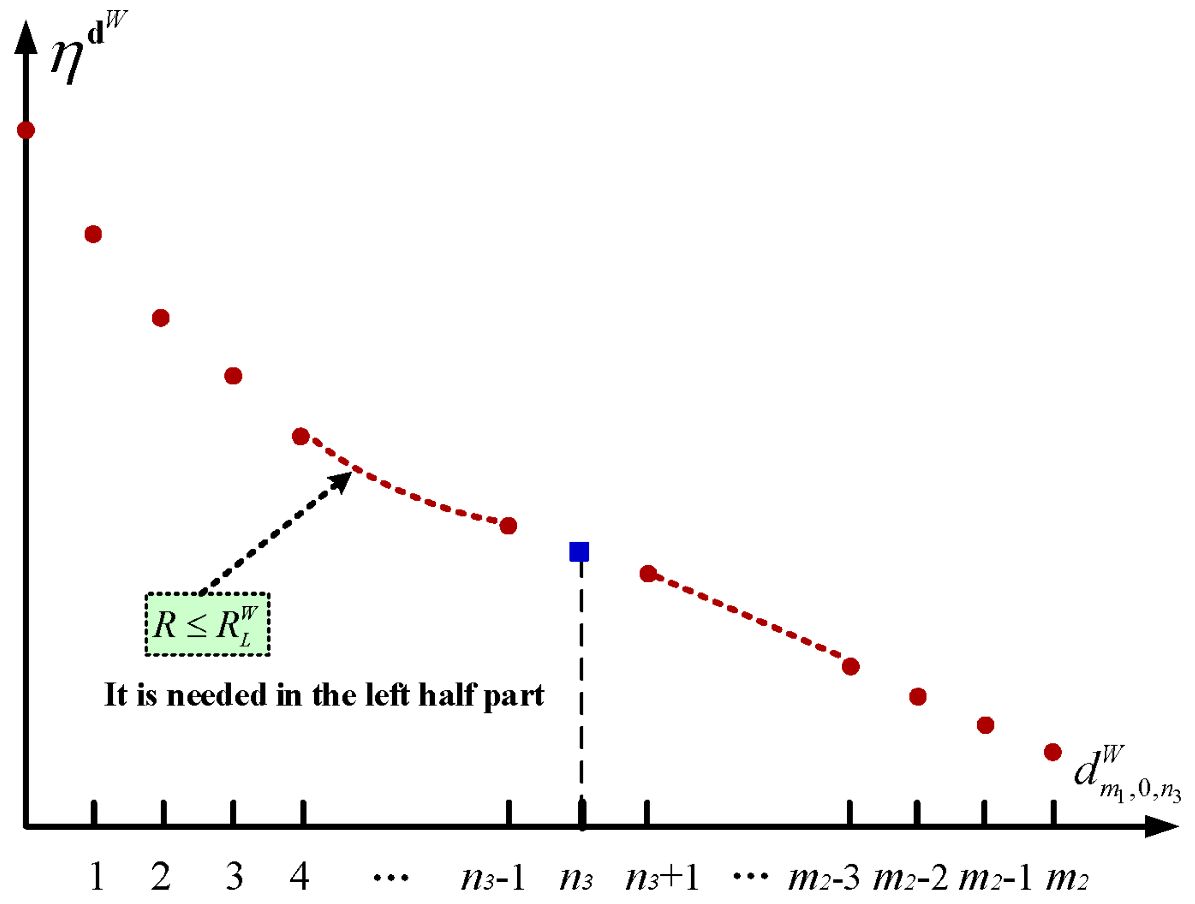
If , for any setup policy with and for each , then the long-run average profit is strictly monotone decreasing with respect to each decision element .
Proof of Theorem 8.
This proof is similar to that of Theorem 5. For each , we consider two setup policies with an interrelated structure as follows:
where , and for . It is clear that
If , then it is seen from Proposition 1 that . Thus, we get that for the two setup policies with and ,
This shows that for ,
This completes the proof. □
When , we also use Figure 4 to provide an intuitive summary for the main results given in Theorems 4 and 8.
6.2.2. The Sleep Policy with
Theorem 9.
If , then for any sleep policy with and for each , , the long-run average profit is strictly monotone increasing with respect to each decision element , for .
Proof of Theorem 9.
This proof is similar to that of Theorem 6. For each and , we consider two sleep policies with an interrelated structure as follows:
where , and . It is clear that
By a similar analysis to that in Theorem 6, if , then it is seen from Proposition 1 that for we have . Thus, we get that for and , is strictly monotone decreasing with respect to , hence it is also strictly monotone increasing with respect to . Thus, we get that for the two sleep policies with and ,
This shows that
This completes the proof. □
When , we also use Figure 5 to provide an intuitive summary for the main results given in Theorem 9.
As a simple summarization of Theorems 8 and 9, the following theorem further describes monotone structure of the long-run average profit with respect to the asynchronous energy-efficient policy, while its proof is easy only through using the condition that makes and .
Theorem 10.
If , then for any asynchronous energy-efficient policy , the long-run average profit is strictly monotone with respect to each decision element of and of , respectively.
In the remainder of this section, we discuss a more complicated case with the service price . In this case, we use the bang–bang control and the asynchronous structure of to prove that the optimal asynchronous energy-efficient polices and both have bang–bang control forms.
6.3. The Service Price
For the price , we can further derive the following theorems about the monotonicity of with respect to the setup policy and the sleep policy, respectively.
6.3.1. The Setup Policy with
For the service price , the following theorem provides the monotonicity of with respect to the decision element .
Theorem 11.
If , then the long-run average profit is monotone (either increasing or decreasing) with respect to the decision element , where and .
Proof of Theorem 11.
Similarly to the first part of the proof for Theorem 5, we consider any two setup policies with an interrelated structure as follows:
where . Applying Lemma 1, we obtain
On the other hand, we can similarly obtain the following difference equation
Therefore, we have the sign conservation equation
The above equation means that the sign of and are always identical when a particular decision element is changed to any . With the sign conservation Equation (44) and the performance difference Equation (43), we can directly derive that the long-run average profit is monotone with respect to . This completes the proof. □
Based on Theorem 11, the following corollary directly derives that the optimal decision element has a bang–bang control form (see more details in Cao [34] and Xia and Chen [35]).
Corollary 1.
For the setup policy, the optimal decision element is either 0 or , i.e., the bang–bang control is optimal.
With Corollary 1, we should either keep all servers in sleep mode or turn on the servers such that the number of working servers equals the number of waiting jobs in the buffer. In addition, we can see that the search space of can be reduced from to a two-element set , which is a significant reduction of search complexity.
6.3.2. The Sleep Policy with
For the service price , the following theorem provides the monotonicity of with respect to the decision element .
Theorem 12.
If , then the long-run average profit is monotone (either increasing or decreasing) with respect to the decision element , where , and .
Proof of Theorem 12.
Similar to the proof for Theorem 11, we consider any two sleep policies with an interrelated structure as follows:
where . Applying Lemma 1, we obtain
On the other hand, we can also obtain the following difference equation:
Thus, the sign conservation equation is given by
This means that the signs of and are always identical when a particular decision element is changed to any . We can directly derive that the long-run average profit is monotone with respect to . This completes the proof. □
Corollary 2.
For the sleep policy, the optimal decision element is either or , i.e., the bang–bang control is optimal.
With Corollary 2, we should either keep all in sleep or turn off the servers such that the number of sleeping servers equals the number of servers without jobs in Group 2. We can see that the search space of can be reduced from to a two-element set , hence this is also a significant reduction of search complexity.
It is seen from Corollaries 1 and 2 that the form of the bang–bang control is very simple and easy to adopt in practice, while the optimality of the bang–bang control guarantees the performance confidence of such simple forms of control. This makes up the threshold-type of the optimal asynchronous energy-efficient policy in the data center.
7. The Maximal Long-Run Average Profit
In this section, we provide the optimal asynchronous dynamic policy of the threshold-type in the energy-efficient data center and further compute the maximal long-run average profit.
We introduce some notation as follows:
Now, we express the optimal asynchronous energy-efficient policy of the threshold-type and compute the maximal long-run average profit under three different service prices as follows:
Case 1.
The service price
It follows from Theorem 7 that
thus we have
Case 2.
The service price
It follows from Theorem 10 that
thus we have
Remark 5.
The above results are intuitive because when the service price is suitably high, the number of working servers is equal to a crucial number related to waiting jobs both in Group 2 and in the buffer; when the service price is lower, each server at the work state must pay a high energy consumption cost, but they receive only a low revenue. In this case, the profit of the data center cannot increase, so that all the servers in Group 2 would like to be closed at the sleep state.
Case 3.
The service price
In Section 6.3, we have, respectively, proven the optimality of the bang–bang control for the setup and sleep policies, regardless of the service price R. However, if , we cannot exactly determine the monotone form (i.e., increasing or decreasing) of the optimal asynchronous energy-efficient policy. This makes the threshold-type of the optimal asynchronous energy-efficient policy in the data center. In fact, such a threshold-type policy also provides us with a choice to compute the optimal setup and sleep policies, they not only have a very simple form but are also widely adopted in numerical applications.
In what follows, we focus our study on the threshold-type asynchronous policy, although its optimality is not yet proven in our next analysis.
We define a couple of threshold-type control parameters as follows:
where and are setup and sleep thresholds, respectively. Furthermore, we introduce two interesting subsets of the policy set . We write as a threshold-type setup policy and as a threshold-type sleep policy. Let
Then
It is easy to see that .
For an asynchronous energy-efficient policy , it follows from (4) to (7) that for and
for , and
for , and
for , and
for , and
for , and ,
Note that
It follows from (48) that the long-run average profit under policy is given by
Let
Then, we call the optimal threshold-type asynchronous energy-efficient policy in the policy set . Since , the partially ordered set shows that is also a partially ordered set. Based on this, it is easy to see from the two partially ordered sets and that
For the energy-efficient data center, if , then we call the optimal threshold-type asynchronous energy-efficient policy in the original policy set ; if , then we call the suboptimal threshold-type asynchronous energy-efficient policy in the original policy set .
Remark 6.
This paper is a special case of the group-server queue (see Li et al. [6]), but it provides a new theoretical framework for the performance optimization of such queueing systems. It is also more applicable to large-scale service systems, such as data centers for efficiently allocating service resources.
Remark 7.
In this paper, we discuss the optimal asynchronous dynamic policy of the energy-efficient data center deeply, and such types of policies are widespread in practice. It would be interesting to extend our results to a more general situation. Although the sensitivity-based optimization theory can effectively overcome the drawbacks of MDPs, it still has some limitations. For example, it cannot discuss the optimization of two or more dynamic control policies synchronously, which is a very important research direction in dynamic optimization.
8. Conclusions
In this paper, we highlight the optimal asynchronous dynamic policy of an energy-efficient data center by applying sensitivity-based optimization theory and RG-factorization. Such an asynchronous policy is more important and necessary in the study of energy-efficient data centers, and it largely makes an optimal analysis of energy-efficient management more interesting, difficult, and challenging. To this end, we consider a more practical model with several basic factors, for example, a finite buffer, a fast setup process from sleep to work, and the necessary cost of transferring jobs from Group 2 either to Group 1 or to the buffer. To find the optimal asynchronous dynamic policy in the energy-efficient data center, we set up a policy-based block-structured Poisson equation and provide an expression for its solution by means of the RG-factorization. Based on this, we derive the monotonicity and optimality of the long-run average profit with respect to the asynchronous dynamic policy under different service prices. We prove the optimality of the bang–bang control, which significantly reduces the action search space, and study the optimal threshold-type asynchronous dynamic policy. Therefore, the results of this paper provide new insights to the discussion of the optimal dynamic control policies of more general energy-efficient data centers.
Along such a line, there are a number of interesting directions for potential future research, for example:
- Analyzing non-Poisson inputs such as Markovian arrival processes (MAPs) and/or non-exponential service times, e.g., the PH distributions;
- Developing effective algorithms for finding the optimal dynamic policies of the policy-based block-structured Markov process (i.e., block-structured MDPs);
- Discussing the fact that the long-run performance is influenced by the concave or convex reward (or cost) function;
- Studying individual optimization for the energy-efficient management of data centers from the perspective of game theory.
Author Contributions
Conceptualization, J.-Y.M. and Q.-L.L.; methodology, L.X. All authors have read and agreed to the published version of the manuscript.
Funding
This research was funded in part by the National Natural Science Foundation of China under grant No. 71932002, by the Beijing Social Science Foundation Research Base Project under grant No. 19JDGLA004, and in part by the National Natural Science Foundation of China under grant No. 61573206 and No. 11931018.
Institutional Review Board Statement
Not applicable.
Informed Consent Statement
Not applicable.
Acknowledgments
The authors are grateful to the editor and anonymous referees for their constructive comments and suggestions, which sufficiently help the authors to improve the presentation of this manuscript.
Conflicts of Interest
The authors declare no conflict of interest.
Appendix A. Special Cases
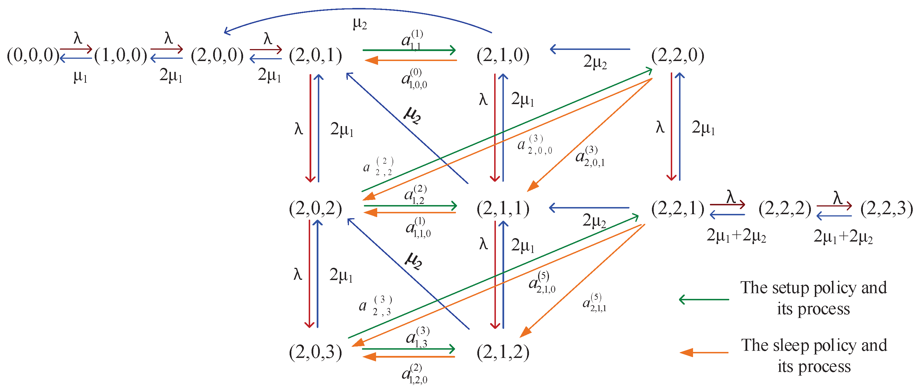
In this appendix, we provide two simple special cases to understand the state transition relations and the infinitesimal generator of the policy-based block-structured continuous-time Markov process .
Case A1.
and
To understand the block-structured continuous-time Markov process under an asynchronous energy-efficient policy, we first take the simplest case of and as an example to illustrate the state transition relations and infinitesimal generator in detail.
Figure A1 shows the arrival and service rates without any policy for the Markov process The transitions in which the transfer rates and the policies are simultaneously involved are a bit difficult, and such transition relations appear in a Markov chain with sync jumps of multi-events (either transition rates or policies (see Budhiraja and Friedlander [40])). For example, what begins a setup policy at State is the entering Poisson process to State , whose inter-entering times are i.i.d. and exponential with the entering rate . Hence, if there exists one or two server set ups, then the transition rate from State to State is . Such an entering process is easy to see in Figure A1.
Figure A1.
State transition relations for the case of and .

We denote as the transitions with the setup policy
Similarly, denotes the transitions with the sleep policy from
Furthermore, we write the diagonal entries
Therefore, its infinitesimal generator is given by
where for level 0, it is easy to see that
for level 1, the setup policy affects the infinitesimal generator
for level 2, the sleep policy affects the infinitesimal generator
for level 3, we have
for level 4, we have
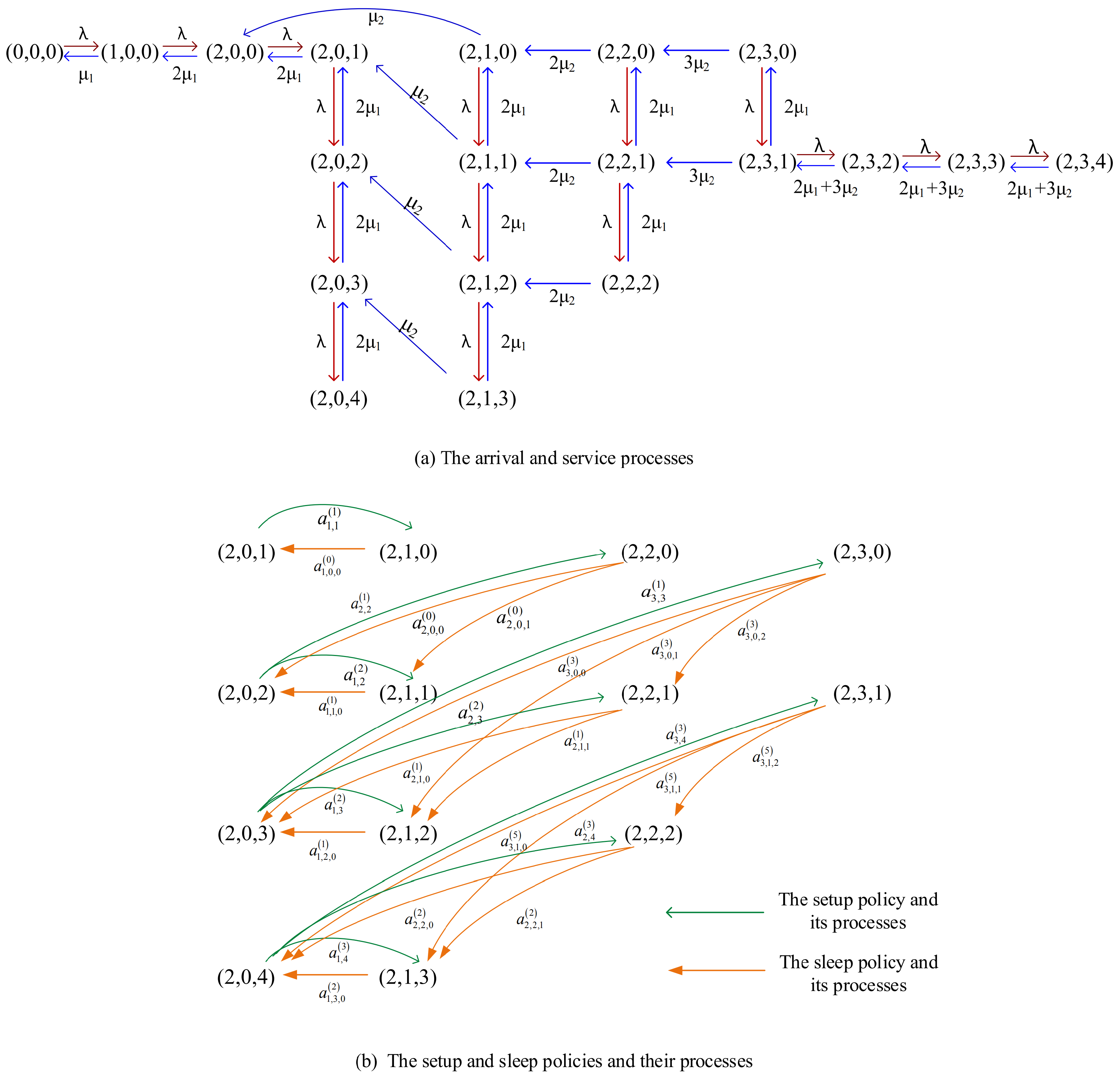
Case A2.
and
To further understand the policy-based block-structured continuous-time Markov process , we take another example to illustrate that if the parameters and increase slightly, the complexity of the state transition relations will increase considerably.
Figure A2.
State transition relations for the case of and .

The number of servers in Group 2 and the buffer capacity both increase by one, which makes the number of state transitions affected by the setup and sleep policies increase from 5 to 9 and from 7 to 15, respectively. Compared with Figure A2, the state transition relations become more complicated. We divide the state transition rate of the Markov process into two parts, as shown in Figure A2: (a) the state transitions without any policy and (b) the state transitions by both setup and sleep policies. Similar to Case 1, for the state transitions in which the transfer rates and the policies are simultaneously involved in the Markov chain with sync jumps of multi-events, the transfer rate is equal to the total entering rate at a certain state.
Furthermore, its infinitesimal generator is given by
Similarly, we can obtain every element here, we omit the computational details.
Appendix B. State Transition Relations
In this appendix, we provide a general expression for the state transition relations of the policy-based block-structured continuous-time Markov process . To express the state transition rates, in what follows, we need to introduce some notations.
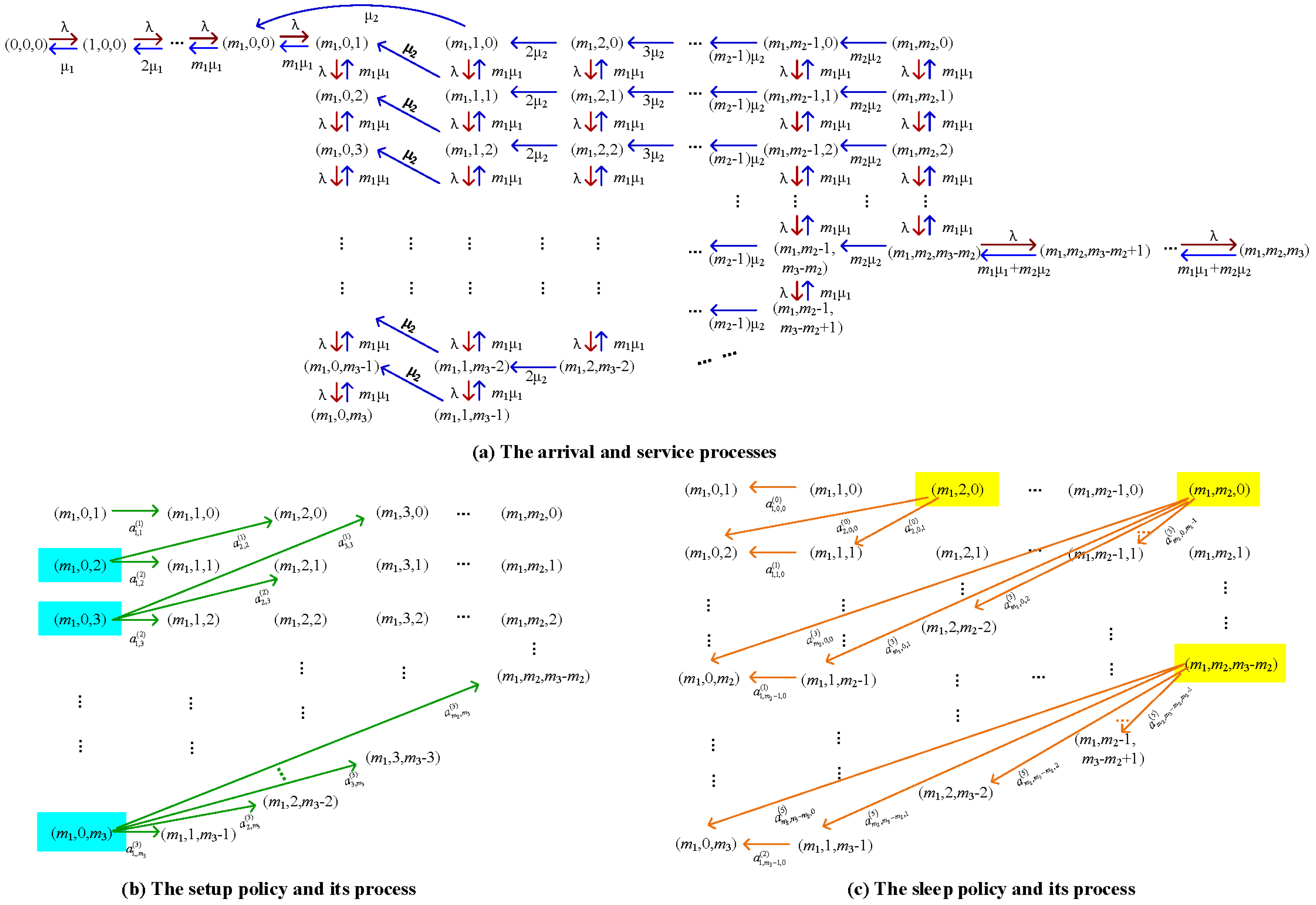
Based on the state transition rates for both special cases that are related to either the arrival and service processes or the setup and sleep policies, Figure A3 provides the state transition relations of the Markov process in general. Note that the figure is so complicated that we have to decompose it into three different parts: (a) the arrival and service processes, (b) the state transitions by the setup policy, and (c) the state transitions by the sleep policy. However, the three parts must be integrated as a whole.
(a) The arrival and service rates: The first type is ordinary for the arrival and service rates without any policy (see Figure A3a).
(b) The setup policy: For we write
for
for
Observing Figure A3b, what begins a setup policy at State is the entering Poisson process to State , whose inter-entering times are i.i.d. and exponential with entering rates, namely either for or for . Such an entering process is easy to see from Figure A3a.
Since the setup and sleep policies are asynchronous, will not contain any transition with the sleep policy because the sleep policy cannot be followed by the setup policy at the same time. To express the diagonal entries of in Appendix C, we introduce
(c) The sleep policy: For and we write
From Figure A3c, it is seen that there is a difference between the sleep and setup policies: State transitions with the sleep policy exist at many states for Clearly, the state transition with the sleep policy from State is the entering Poisson processes, with the rate being the total entering rate to State Note that the sleep policy cannot be followed by the setup policy at the same time. Thus, it is easy to check these state transition rates given in the above ones.
To express the diagonal entries of for , we introduce
Remark A1.
The first key step in applications of the sensitivity-based optimization to the study of energy-efficient data centers is to draw the state transition relation figure (e.g., see Figure A3) and to write the infinitesimal generator of the policy-based block-structured Markov process. Although this paper has largely simplified the model assumptions, Figure A3 is still slightly complicated by its three separate parts: (a), (b), and (c). Obviously, if we consider some more general assumptions (for example, (i) the faster servers are not cheaper, (ii) Group 2 is not slower, (iii) there is no transfer rule, and so on), then the state transition relation figure will become more complicated, so that it is more difficult to write the infinitesimal generator of the policy-based block-structured Markov process and to solve the block-structured Poisson equation.
Figure A3.
State transition relations of the policy-based block-structured Markov process.

Remark A2.
Figure A3 shows that Part (a) expresses the arrival and service rates, while Parts (b) and (c) express the state transition rates caused by the setup and sleep policies, respectively. Note that the setup policy is started by only the arrival and service process at State for (see Part (b)), in which there is no setup rate because the setup time is so short that it is ignored. Similarly, it is easy to understand Part (c) for the sleep policy. It is worthwhile to note that an idle server may be at the work state, as seen in the idle servers with the work state in Group 1.
Appendix C. Block Elements in Q(d)
In this appendix, we write each block element in the matrix .
(a) For level 0, it is easy to see that
(b) For level 1, the setup policy affects the infinitesimal generator, and is given by
where
and is a block of zeros with suitable size. From (A1), we have
(c) For level 2, i.e., ,
and
(d) For level , , subdivided into three cases as follows:
For ,
where
For
For
(e) For level , i.e.,
where
and
(f) For level ,
where
References
- Masanet, E.; Shehabi, A.; Lei, N.; Smith, S.; Koomey, J. Recalibrating global data center energy-use estimates. Science 2020, 367, 984–986. [Google Scholar] [CrossRef] [PubMed]
- Zhang, Q.; Meng, Z.; Hong, X.; Zhan, Y.; Liu, J.; Dong, J.; Bai, T.; Niu, J.; Deen, M.J. A survey on data center cooling systems: Technology, power consumption modeling and control strategy optimization. J. Syst. Archit. 2021, 119, 102253. [Google Scholar] [CrossRef]
- Nadjahi, C.; Louahlia, H.; Lemasson, S. A review of thermal management and innovative cooling strategies for data center. Sustain. Comput. Inform. Syst. 2018, 19, 14–28. [Google Scholar] [CrossRef]
- Koot, M.; Wijnhoven, F. Usage impact on data center electricity needs: A system dynamic forecasting model. Appl. Energy 2021, 291, 116798. [Google Scholar] [CrossRef]
- Shirmarz, A.; Ghaffari, A. Performance issues and solutions in SDN-based data center: A survey. J. Supercomput. 2020, 76, 7545–7593. [Google Scholar] [CrossRef]
- Li, Q.L.; Ma, J.Y.; Xie, M.Z.; Xia, L. Group-server queues. In Proceedings of the International Conference on Queueing Theory and Network Applications, Qinhuangdao, China, 21–23 August 2017; pp. 49–72. [Google Scholar]
- Harchol-Balter, M. Open problems in queueing theory inspired by data center computing. Queueing Syst. 2021, 97, 3–37. [Google Scholar] [CrossRef]
- Barroso, L.A.; Hölzle, U. The case for energy-proportional computing. Computer 2007, 40, 33–37. [Google Scholar] [CrossRef]
- Kuehn, P.J.; Mashaly, M.E. Automatic energy efficiency management of data center resources by load-dependent server activation and sleep modes. Ad Hoc Netw. 2015, 25, 497–504. [Google Scholar] [CrossRef]
- Gandhi, A. Dynamic Server Provisioning for Data Center Power Management. Ph.D. Thesis, School of Computer Science, Carnegie Mellon University, Pittsburgh, PA, USA, 2013. [Google Scholar]
- Gandhi, A.; Doroudi, S.; Harchol-Balter, M.; Scheller-Wolf, A. Exact analysis of the M/M/k/setup class of Markov chains via recursive renewal reward. Queueing Syst. 2014, 77, 177–209. [Google Scholar] [CrossRef]
- Gandhi, A.; Gupta, V.; Harchol-Balter, M.; Kozuch, M.A. Optimality analysis of energy-performance trade-off for server farm management. Perform. Eval. 2010, 67, 1155–1171. [Google Scholar] [CrossRef] [Green Version]
- Gandhi, A.; Harchol-Balter, M.; Adan, I. Server farms with setup costs. Perform. Eval. 2010, 67, 1123–1138. [Google Scholar] [CrossRef]
- Maccio, V.J.; Down, D.G. On optimal policies for energy-aware servers. Perform. Eval. 2015, 90, 36–52. [Google Scholar] [CrossRef] [Green Version]
- Maccio, V.J.; Down, D.G. Exact analysis of energy-aware multiserver queueing systems with setup times. In Proceedings of the IEEE 24th International Symposium on Modeling, Analysis and Simulation of Computer and Telecommunication Systems, London, UK, 19–21 September 2016; pp. 11–20. [Google Scholar]
- Phung-Duc, T. Exact solutions for M/M/c/setup queues. Telecommun. Syst. 2017, 64, 309–324. [Google Scholar] [CrossRef] [Green Version]
- Phung-Duc, T.; Kawanishi, K.I. Energy-aware data centers with s-staggered setup and abandonment. In Proceedings of the International Conference on Analytical and Stochastic Modeling Techniques and Applications, Cardiff, UK, 24–26 August 2016; pp. 269–283. [Google Scholar]
- Gebrehiwot, M.E.; Aalto, S.; Lassila, P. Optimal energy-aware control policies for FIFO servers. Perform. Eval. 2016, 103, 41–59. [Google Scholar] [CrossRef]
- Gebrehiwot, M.E.; Aalto, S.; Lassila, P. Energy-performance trade-off for processor sharing queues with setup delay. Oper. Res. Lett. 2016, 44, 101–106. [Google Scholar] [CrossRef]
- Gebrehiwot, M.E.; Aalto, S.; Lassila, P. Energy-aware SRPT server with batch arrivals: Analysis and optimization. Perform. Eval. 2017, 15, 92–107. [Google Scholar] [CrossRef]
- Mitrani, I. Service center trade-offs between customer impatience and power consumption. Perform. Eval. 2011, 68, 1222–1231. [Google Scholar] [CrossRef]
- Mitrani, I. Managing performance and power consumption in a server farm. Ann. Oper. Res. 2013, 202, 121–134. [Google Scholar] [CrossRef]
- Kamitsos, I.; Ha, S.; Andrew, L.L.; Bawa, J.; Butnariu, D.; Kim, H.; Chiang, M. Optimal sleeping: Models and experiments for energy-delay tradeoff. Int. J. Syst. Sci. Oper. Logist. 2017, 4, 356–371. [Google Scholar] [CrossRef]
- Hipp, S.K.; Holzbaur, U.D. Decision processes with monotone hysteretic policies. Oper. Res. 1988, 36, 585–588. [Google Scholar] [CrossRef]
- Lu, F.V.; Serfozo, R.F. M/M/1 queueing decision processes with monotone hysteretic optimal policies. Oper. Res. 1984, 32, 1116–1132. [Google Scholar] [CrossRef]
- Yang, J.; Zhang, S.; Wu, X.; Ran, Y.; Xi, H. Online learning-based server provisioning for electricity cost reduction in data center. IEEE Trans. Control Syst. Technol. 2017, 25, 1044–1051. [Google Scholar] [CrossRef]
- Ding, D.; Fan, X.; Zhao, Y.; Kang, K.; Yin, Q.; Zeng, J. Q-learning based dynamic task scheduling for energy-efficient cloud computing. Future Gener. Comput. Syst. 2020, 108, 361–371. [Google Scholar] [CrossRef]
- Liang, Y.; Lu, M.; Shen, Z.J.M.; Tang, R. Data center network design for internet-related services and cloud computing. Prod. Oper. Manag. 2021, 30, 2077–2101. [Google Scholar] [CrossRef]
- Xia, L.; Chen, S. Dynamic pricing control for open queueing networks. IEEE Trans. Autom. Control 2018, 63, 3290–3300. [Google Scholar] [CrossRef]
- Xia, L.; Miller, D.; Zhou, Z.; Bambos, N. Service rate control of tandem queues with power constraints. IEEE Trans. Autom. Control 2017, 62, 5111–5123. [Google Scholar] [CrossRef]
- Ma, J.Y.; Xia, L.; Li, Q.L. Optimal energy-efficient policies for data centers through sensitivity-based optimization. Discrete Event Dyn. Syst. 2019, 29, 567–606. [Google Scholar] [CrossRef] [Green Version]
- Chi, C.; Ji, K.; Marahatta, A.; Song, P.; Zhang, F.; Liu, Z. Jointly optimizing the IT and cooling systems for data center energy efficiency based on multi-agent deep reinforcement learning. In Proceedings of the 11th ACM International Conference on Future Energy Systems, Virtual Event, Australia, 22–26 June 2020; pp. 489–495. [Google Scholar]
- Li, Q.L. Constructive Computation in Stochastic Models with Applications: The RG-Factorizations; Springer: Beijing, China, 2010. [Google Scholar]
- Cao, X.R. Stochastic Learning and Optimization—A Sensitivity-Based Approach; Springer: New York, NY, USA, 2007. [Google Scholar]
- Xia, L.; Zhang, Z.G.; Li, Q.L. A c/μ-rule for for job assignment in heterogeneous group-server queues. Prod. Oper. Manag. 2021, 1–18. [Google Scholar] [CrossRef]
- Li, Q.L.; Li, Y.M.; Ma, J.Y.; Liu, H.L. A complete algebraic transformational solution for the optimal dynamic policy in inventory rationing across two demand classes. arXiv 2019, arXiv:1908.09295v1. [Google Scholar]
- Ma, J.Y.; Li, Q.L. Sensitivity-based optimization for blockchain selfish mining. In Proceedings of the International Conference on Algorithmic Aspects of Information and Management, Dallas, TX, USA, 20–22 December 2021; pp. 329–343. [Google Scholar]
- Xia, L. Risk-sensitive Markov decision processes with combined metrics of mean and variance. Prod. Oper. Manag. 2020, 29, 2808–2827. [Google Scholar] [CrossRef]
- Puterman, M.L. Markov Decision Processes: Discrete Stochastic Dynamic Programming; John Wiley& Sons: New York, NY, USA, 2014. [Google Scholar]
- Budhiraja, A.; Friedlander, E. Diffusion approximations for controlled weakly interacting large finite state systems with simultaneous jumps. Ann. Appl. Probab. 2018, 28, 204–249. [Google Scholar] [CrossRef] [Green Version]
Figure 1.
Energy-efficient management of a data center.

Figure 2.
The unimodal structure of the long-run average profit by the setup policy.

Figure 3.
The monotone structure of the long-run average profit by the sleep policy.

Figure 4.
The decreasing structure of the long-run average profit by the setup policy.

Figure 5.
The increasing structure of the long-run average profit by the sleep policy.


Table 1.
Cost notation in the data center.
| Cost | Necessary Interpretation |
|---|---|
| The power consumption price | |
| The holding cost for a job in Group 1 per unit of sojourn time | |
| The holding cost for a job in Group 2 per unit of sojourn time | |
| The holding cost for a job in the buffer per unit of sojourn time | |
| The setup cost for a server switching from the sleep state to the work state | |
| The transferred cost for a incomplete-service job returning to the buffer | |
| The transferred cost for a job in Group 2 is transferred to Group 1 | |
| The opportunity cost for each lost job | |
| R | The service price from the served job |
Publisher’s Note: MDPI stays neutral with regard to jurisdictional claims in published maps and institutional affiliations. |
© 2022 by the authors. Licensee MDPI, Basel, Switzerland. This article is an open access article distributed under the terms and conditions of the Creative Commons Attribution (CC BY) license (https://creativecommons.org/licenses/by/4.0/).
Share and Cite
MDPI and ACS Style
Ma, J.-Y.; Li, Q.-L.; Xia, L. Optimal Asynchronous Dynamic Policies in Energy-Efficient Data Centers. Systems 2022, 10, 27. https://0-doi-org.brum.beds.ac.uk/10.3390/systems10020027
AMA Style
Ma J-Y, Li Q-L, Xia L. Optimal Asynchronous Dynamic Policies in Energy-Efficient Data Centers. Systems. 2022; 10(2):27. https://0-doi-org.brum.beds.ac.uk/10.3390/systems10020027
Chicago/Turabian StyleMa, Jing-Yu, Quan-Lin Li, and Li Xia. 2022. "Optimal Asynchronous Dynamic Policies in Energy-Efficient Data Centers" Systems 10, no. 2: 27. https://0-doi-org.brum.beds.ac.uk/10.3390/systems10020027
Note that from the first issue of 2016, this journal uses article numbers instead of page numbers. See further details here.