Categorification of the Müller-Wichards System Performance Estimation Model: Model Symmetries, Invariants, and Closed Forms

1
Electromagnetic and Sensor Systems Department, Naval Surface Warfare Center Dahlgren Division, Dahlgren, VA 22448, USA
2
Strategic and Computing Systems Department, Naval Surface Warfare Center Dahlgren Division, Dahlgren, VA 22448, USA
*
Author to whom correspondence should be addressed.
Systems 2019, 7(1), 6; https://0-doi-org.brum.beds.ac.uk/10.3390/systems7010006
Submission received: 25 October 2018
/
Revised: 11 December 2018
/
Accepted: 11 December 2018
/
Published: 24 January 2019
(This article belongs to the Special Issue Reliability and Maintenance Scheduling: Methods, Theory and applications)
Abstract
:The Müller-Wichards model (MW) is an algebraic method that quantitatively estimates the performance of sequential and/or parallel computer applications. Because of category theory’s expressive power and mathematical precision, a category theoretic reformulation of MW, i.e., CMW, is presented in this paper. The CMW is effectively numerically equivalent to MW and can be used to estimate the performance of any system that can be represented as numerical sequences of arithmetic, data movement, and delay processes. The CMW fundamental symmetry group is introduced and CMW’s category theoretic formalism is used to facilitate the identification of associated model invariants. The formalism also yields a natural approach to dividing systems into subsystems in a manner that preserves performance. Closed form models are developed and studied statistically, and special case closed form models are used to abstractly quantify the effect of parallelization upon processing time vs. loading, as well as to establish a system performance stationary action principle.
1. Introduction
In the late 1980s, D. Müller-Wichards proposed a concise novel approach for estimating the total performance of computer-based (but machine independent) applications by algebraically combining the known performance estimates of the individual arithmetic, data movement, and delay elements that comprise the applications in a manner that also accounts for various degrees of parallelism that can occur during processing [1]. The essence of the mathematical framework upon which the Müller-Wichards model (MW) is based is abstracted by the expression , where is a monoid (i.e., a semigroup with identity) representation of the application, is the Müller-Wichards performance algebra (also a monoid), and is a monoid homomorphism. The image in of a single application element in provides a numerical performance measure for . The total numerical performance estimate for the application results naturally from the associative binary operations in and and the homomorphism property of , which algebraically combines the performance estimates for each application element in .
Every area of mathematics (e.g., group theory, topology) is described by numerous definitions, theorems, and constructions. However, many common mathematical concepts occur naturally with only slight variation in the various areas of mathematics. Category theory is that branch of mathematics which identifies and studies these common concepts and provides formal mechanisms for mapping them from one area of mathematics to another. More specifically, a category (e.g., the category of sets) consists of a class of objects (e.g., sets), morphisms between objects (e.g., maps between sets), an identity morphism for each object (e.g., the set identity map), and a rule for associatively composing morphisms (e.g., composition of maps). Functors provide formal maps between categories (e.g., from the category of groups to the category of sets) by associating objects and morphisms in different categories subject to the constraints that morphism composition and object identities are preserved.
Because of its generality category, theory has found application in recent years in such diverse areas as physics (e.g., [2,3,4,5]), design specification (e.g., [6,7]), data fusion (e.g., [8]), computer science (e.g., [9]), computer security (e.g., [10,11]), systems engineering (e.g., [12]), manufacturing (e.g., [13]), theoretical biology (e.g., [14,15,16]), network theory (e.g., [17]), multi-agent systems models (e.g., [18]), concurrent system design verification (e.g., [19]), emergence (e.g., [20]), and artificial general intelligence (e.g., [21]). Motivated by category theory’s mathematical precision and expressive power, this paper introduces a new category theoretic application useful for numerical systems engineering modelling and analysis via a very simple straightforward categorification of MW for the case that the application monoid is a free monoid generated by a finite set of basis processes, i.e., is the set of all finite sequences of basis processes, including the empty sequence-where each sequence represents a system and each basis process corresponds to either an arithmetic process, a data movement process, or a delay process-and catenation of systems serves as the associative binary operation. The categorified MW-denoted by CMW-is comprised of three components: a single object category of systems that is specified by and has elements of as its set of morphisms; a single object performance category that is specified by and has the elements of as its set of morphisms; and a performance functor specified by with the category of systems as its domain and the performance category as its codomain.
CMW is effectively numerically equivalent to MW with the added benefit that the formalism introduced by categorification provides a precise vocabulary useful for identifying and discussing certain fundamental properties of both the model and the systems modelled by it. In particular, the CMW fundamental symmetry group is introduced and the category theoretic formalism is used to facilitate the identification of associated symmetry invariants found in the model. In addition, the formalism provides a natural approach to system factorization-i.e., dividing a system into subsystems in a manner that maintains its integrity-i.e., preserves the performance of the undivided system.
As indicated above, the objective of this paper is to provide a categorified version of the MW model and exploit the associated category theoretic vocabulary to provide additional insights into properties of the MW model, as well as the systems modelled by it. In order to make this paper reasonably self-contained, relevant definitions, terminology, and preliminary lemmas are summarized in the next section (for additional depth and clarification the reader is invited to consult such references as [22,23,24]). The remainder of this paper is organized as follows: The Müller-Wichards performance categories are defined, and their category theoretic properties discussed in Section 3. The category of systems and the Müller-Wichards performance functors are introduced in Section 4. The CMW fundamental symmetry group is defined and its associated model invariants are identified in Section 5. System factorization and a “product of categories” performance model are discussed in Section 6. Closed form models are developed in Section 7 and several aspects of closed form models are studied statistically in Section 8. Special case closed form models are developed in Section 9. These special case closed form models are applied in Section 10 to abstractly demonstrate the effect of parallelization on system processing time vs. loading and to obtain a stationary action principle for system performance. Concluding remarks comprise the final section of this paper. To avoid disrupting the flow of the text, proofs for all theorems (including those for the special case closed form models) are consigned to Appendix A.
2. Definitions, Terminology, and Preliminary Lemmas
2.1. Categories and Morphisms
- For every pair of objects there is a (possibly empty) set of morphisms from to ;
- For any there is a composition “” of morphismsgiven by with the properties:
- For every there is an identity morphism such that for and , and ;
- When defined, composition of morphisms is associative, i.e., .
To illustrate this definition, consider the following canonical examples of categories:
- The category where is the collection of all sets, the morphisms are the ordinary mappings between sets, and is the usual composition of maps.
- The category where is the collection of all groups, the morphisms are the ordinary group homomorphisms, and is the usual composition of homomorphisms.
It is easily verified that and Grp satisfy items 3 and 4 above.
A category is a subcategory of a category if ([22], p. 7): every object of is an object of ; for all objects of , ; the composition of two morphisms in is the same as their composition in ; and for all objects of , is the same in as it is in . If is a set, then is a small category ([22], p. 6) and if for all , then is a connected category ([22], p. 19).
Morphisms are classified in a variety of ways according to their composition properties. Of interest here are monic and epic morphisms. A morphism is monic ([22], p. 11) if implies and it is epic ([22], p. 12) if implies . For example, in the category injective maps are monic morphisms and surjective maps are epic morphisms. A morphism that is both monic and epic is a bimorphism ([22], p. 15). A morphism is factorizable ([22], p. 43) if , where is monic and is epic.
Another useful notion involving morphisms is the sieve ([25], p. 206) on an object. For some consider the set of morphisms and observe that is closed under left composition, i.e., when and for any . An sieve is the subset that is closed under left composition, i.e., when . Note that there are at least two sieves for every , namely and the empty sieve .
2.2. Functors
Functors can be regarded as morphisms between categories and-in a sense-they provide a “picture” of what one category looks like in another. If is a covariant functor-or simply a functor (contravariant functors are not used here) ([22], p. 73)-from category to category (denoted ), then it assigns to every an and to every an such that:
- for every ; and
- When is defined in , then is defined in and .
is full ([22], p. 97) if for all the mapping defined by is surjective, and is faithful ([22], p. 97) if this mapping is injective. Simple examples of functors include:
- The identity functor which makes the assignments for every and for every .
- The forgetful functor which assigns to every group its underlying set and to each homomorphism the set map (i.e., forgets group structure going from to ).
It can be determined by inspection that these functors satisfy the required properties given above by items 1 and 2.
Preservation and reflection are two important features of functors. A functor preserves a categorical property ([22], p. 97) if-whenever an object, morphism, or diagram has property in , then the image under of that object, morphism, or diagram has property in . Similarly, reflects property ([22], p. 97) if-whenever the image under of an object, morphism, or diagram has property in , then that object, morphism, or diagram has property in .
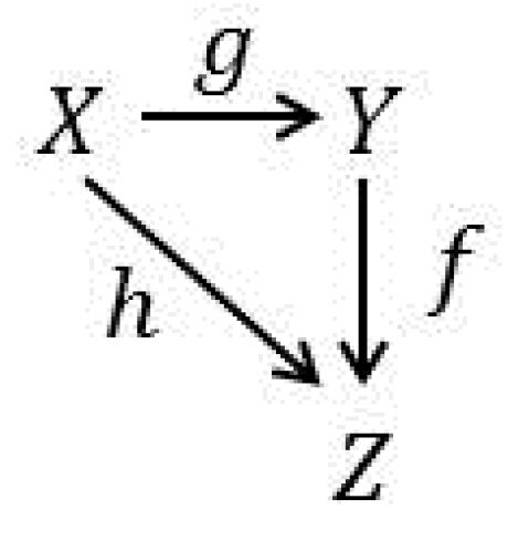
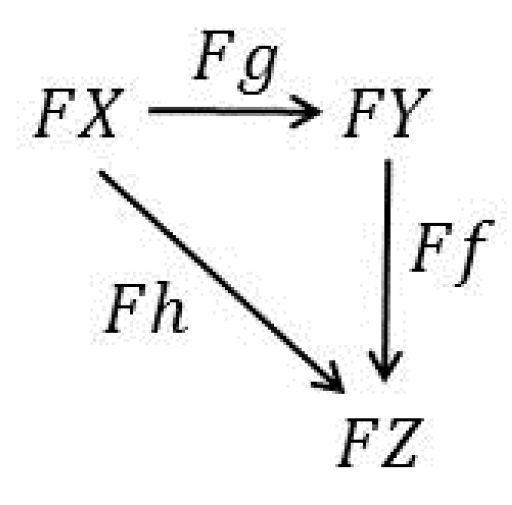
It is readily deduced from item (2) that, in general, functors preserve commutative triangles of morphisms. For example, if Figure 1 is the commutative triangle for in , then it must be
the case that the commutative triangle in Figure 2 is the preserved image of Figure 1 under the functor:
in . Note that Figure 1 is a factorization of when is monic and is epic.
2.3. Preliminary Lemmas
The following lemmas are needed to prove and discuss the main results of this paper. They have been established elsewhere and are stated here without proof for the reader’s convenience.
Lemma 1 [9].
Any monoidspecifies a categorywithas its only object, the elements ofas its only set of morphisms, and the binary operation onas its composition of morphisms.
Lemma 2 [9].
Each monoid homomorphismspecifies a functorwithand Fxforsuch thatinwhenin.
Lemma 3 [24].
Letbe the free monoid on a setandbe any monoid. Ifis any mapping ofinto, thencan be extended in one and only one way to a homomorphismofintoas.
Lemma 4 [22].
Every faithful functor reflects monics, epics, and commutative triangles.
Lemma 5 [24].
A free monoidis cancellative (i.e., and implies for) and equidivisible (i.e., implies there exists an such that either and or and for).
As an example of equidivisibility, suppose is a commutative square in a free monoid with , , , and . Then there exists an such that and .
3. The Müller-Wichards Performance Categories
As mentioned in the introduction, in 1988 Dieter Müller-Wichards posited a (computing) machine independent “performance algebra” designed to estimate the total performance of a specific implementation of an application on a machine using the (known) performance characteristics of its individual building blocks. This approach enabled trade-off studies and analyses of applications using its various decompositions and implementations [1]. As indicated above, similar studies and analyses can be performed using CMW to estimate the numerical performance of any system that can be represented as sequences of arithmetic, data movement, and delay processes.
The Müller-Wichards performance algebra consists of a set whose elements are ordered in triples along with an associative binary operation, which defines how the elements of the set are to be multiplied. These elements are partitioned into three distinct subsets depending upon whether they are arithmetic, data movement, or delay elements. The first and second entries in each triple correspond to a performance value (e.g., a processing or data movement rate) and a weight value (e.g., the number of operations to be performed or the amount of data to be moved), respectively (delay elements are a special case—see below). The third entry is either a -which defines the element as a data movement or delay element-or a -which defines the element as an arithmetic element. Multiplication of an arithmetic element by any element produces another arithmetic element, whereas the product of a data movement element with a data movement element or a delay element is a data movement element. The set of delay elements is closed under this multiplication.
Multiplication is defined in terms of a positive real valued parameter , which provides a family of (“skewed” time) results that interpolate between completely sequential and completely parallel execution of the associated application. The value of this parameter can be selected to account for execution time “speedup” or for degrees of machine and application parallelism.
The sets that define the Müller-Wichards performance algebra are:
where ,
and
Each element in and is a triple , where is a performance value, is a weight value, and determines the element type (i.e., , , or ).
Let and define the operation as follows:
- If and , then , whereand
- If , then where and are given by Equations and , respectively.
The elements are comparable if or or . If , then when are comparable and either or and .
Theorem 1.
is a commutative monoidwith identity.
Since is the monoid , then specifies a category according to the prescription given by the next theorem.
Theorem 2.
specifies the Müller-Wichards performance categorywithas its only object,as its only morphism set, and composition of morphisms defined by.
In order to identify additional categorical properties derived from the algebraic structure of , let , and .
Theorem 3.
, are submonoids of.
This leads to the following result:
Theorem 4.
If, thenspecifies the Müller-Wichards performance categorywithas its only object,as its only morphism set, and composition of morphisms defined by.
Note that although , is not a subcategory of because .
Theorem 5.
Each of the categoriesandare small and connected.
Theorem 6.
Every morphism inis a bimorphism.
The following result is included for completeness and is a category theoretic statement of the fact that multiplication in the performance algebra is biased towards arithmetic elements, i.e., the product of any element in set with an element in set is an element in .
Theorem 7.
The setis an- sieve in category.
4. The Category of Systems and the Müller-Wichards Performance Functors
In this section, the category of systems is obtained from the free monoid generated by a finite set of basis processes. Although this approach is similar to that employed in [1] to define , for simplicity the catenation operation in is used here instead of the two operations and used in to distinguish between portions of an application that have sequential and parallel implementations. A product of categories construction will be introduced for this purpose in Section 6.
Recall from Section 1 that consists of all finite sequences of basis processes of The catenation of systems is the system and and are subsystems of . The empty system is the system with no basis processes and serves as the identity element for with .
The category of systems associated with a basis process set is obtained from , as prescribed in the following theorem.
Theorem 8.
specifies the category of systemswithas its only object,as its only morphism set, and composition of morphisms defined by catenation of systems.
Thus, a morphism in is a system and composition of morphisms in is catenation of systems.
Theorem 9.
is a small connected category.
Theorem 10.
Every morphism inis a bimorphism.
Any functor from into or is referred to here as a Müller-Wichards performance functor for and the performance for any system in is its image under a Müller-Wichards performance functor in or . These functors are defined by unique extensions of gauge maps from the set of basis processes into the associated Müller-Wichards performance monoids as described by the following theorem (here “gauge” emphasizes the fact that these maps set the performance gauge for each basis process).
Theorem 11.
For any gauge map [] there is a unique Müller-Wichards performance functor such that
where .
5. The CMW Fundamental Symmetry Group and Associated Invariants
Based upon the discussion above, it is clear that CMW can be abstracted by the functor expressions and . In this section, the CMW fundamental symmetry group is introduced and associated model invariants (which at an abstract level can be viewed as invariants of the modelled system) are identified. Recall that, in general, a symmetry associated with a “situation” is related to an “immunity to change” for some aspect of the “situation”. In order for a “situation” to have a symmetry: (i) the aspect of the “situation” remains unchanged or invariant, when a change or symmetry transformation acts upon the “situation”; and (ii) it must be possible to perform the change, although the change does not actually have to be performed [26]. Here, symmetry and symmetry transformation are used interchangeably.
An automorphism of is a bijection , which preserves the catenation operation in . Since remains unchanged under and it is possible-but not necessary-to apply , then items (i) and (ii) above are satisfied and is a symmetry. The set of all such symmetries under the operation composition of bijections forms the automorphism group ). This group is the CMW fundamental symmetry group.
Theorem 12.
The CMW fundamental symmetry group is isomorphic to the group of permutations of the setof basis processes.
The following corollary is obvious and is stated without proof.
Corollary 1.
A CMW invariant is a CMW property that remains unchanged after every symmetry in the CMW fundamental symmetry group has been applied to .
Theorem 13.
The images ofinandunder the Müller-Wichards performance functorsandrespectively, are CMW invariants.
Theorem 14.
Ifis a commutative triangle in, thenand its image under Müller-Wichards performance functors are CMW invariants.
6. System Factorization and Product Performance Models
Recall from Section 2 that a morphism is factorizable if , where is a monic morphism and is an epic morphism. In the category of systems, this means that when a system is factorizable as , then can be divided into the two subsystems and without affecting the order and content of the base processes in . The integrity of a factorization is maintained if the performance of is identical to that of .
Theorem 15.
Every commutative triangle incorresponds to a system factorization, which maintains its integrity.
A commutative square in corresponds to an equation , where .
Theorem 16.
For every commutative square inthere are two systems in the square, which have factorizations that maintain their integrity.
Corollary 2.
Wheneveris a commutative square in, then eitherandorandare factorizable in,
Corollary 3.
If, thenis factorizable inand maintains its integrity whenis faithful.
Results similar to Corollary 3 also apply for .
Additional modelling flexibility can be obtained using products of categories when a system is comprised of subsystems that have different sequential and/or parallel characteristics. Here, two basis sets and of processes and two morphism compositions and form the product category of systems and the associated Müller-Wichards product performance category , respectively. For the product category the single object is the pair the set of morphisms are ordered pairs such that for , and with composition performed component wise. Similarly, for the product category the object is the pair , the set of morphisms are ordered pairs such that for , and with composition performed component wise. It is easily verified that and are categories where and are the object identities.
Now use the gauge maps and to define as such that and for , . It is readily seen that is a functor because and for , if, then .
Thus:
Of course, a similar construction can be made using products of a finite number of categories of systems and Müller-Wichards performance categories.
Thus, generally distinct performance triples and are obtained, which yield separate performance estimates for systems comprised of basis processes and for systems comprised of basis processes, respectively. Obviously, unless , and cannot be properly combined algebraically to obtain a single performance estimate for a process comprised of both and basis processes. However, an inequality can be established by letting and in Lemma 2.6 in [1]. These yields when . An alternative approach is to estimate the combined processing time for systems composed of processes and for systems composed of processes from and using , where and .
7. Closed Form Models
In this section, the above theory is used to develop general closed form system performance estimation models where a system’s performance and weight are explicit functions of the performances and weights of the processes that comprise the system. The next theorem provides models for systems comprised entirely of a finite number of arithmetic processes or data movement processes. In what follows, let .
Theorem 17.
LetIforthen
whereorwhenor, respectively,, and
Now consider systems comprised entirely of a finite number of delay processes.
Theorem 18.
LetIfthen
where
The last two theorems can be used to construct closed form models for systems comprised of finite numbers of arithmetic, data movement, and delay processes.
Theorem 19.
Suppose the systemis comprised ofarithmetic processes,data movement processes, anddelay processes such that. Then
where
withandgiven by Theorem 17 whenandandgiven by Theorem 17 whenandandgiven by Theorem 18 when.
8. Statistical Properties of for Closed Form Models
Since system performance studies are often stochastic in nature, it is instructive to examine the statistical characteristics of the system performance variable for several cases using the closed form models of Theorem 17 for arithmetic and data movement elements.
8.1. Fixed Rates and Independent Random Weights
Assume that for both element types each rate where is a fixed value, and each weight is an independent random variable described by the same Poisson distribution with mean . In this case-for a fixed , , and λ-Equation (15) can be written as:
Note that it necessarily follows that is also Poisson distributed with mean .
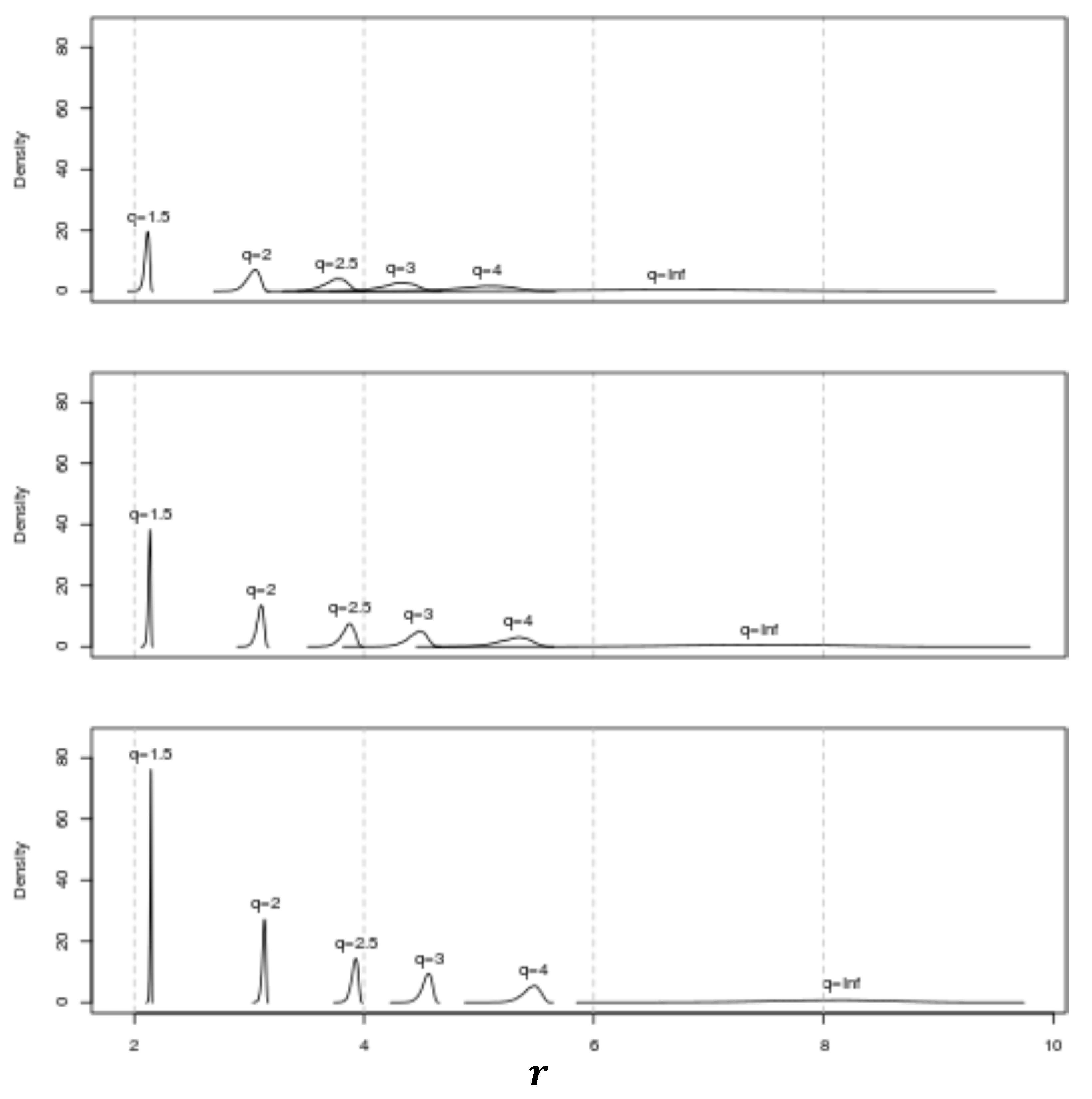
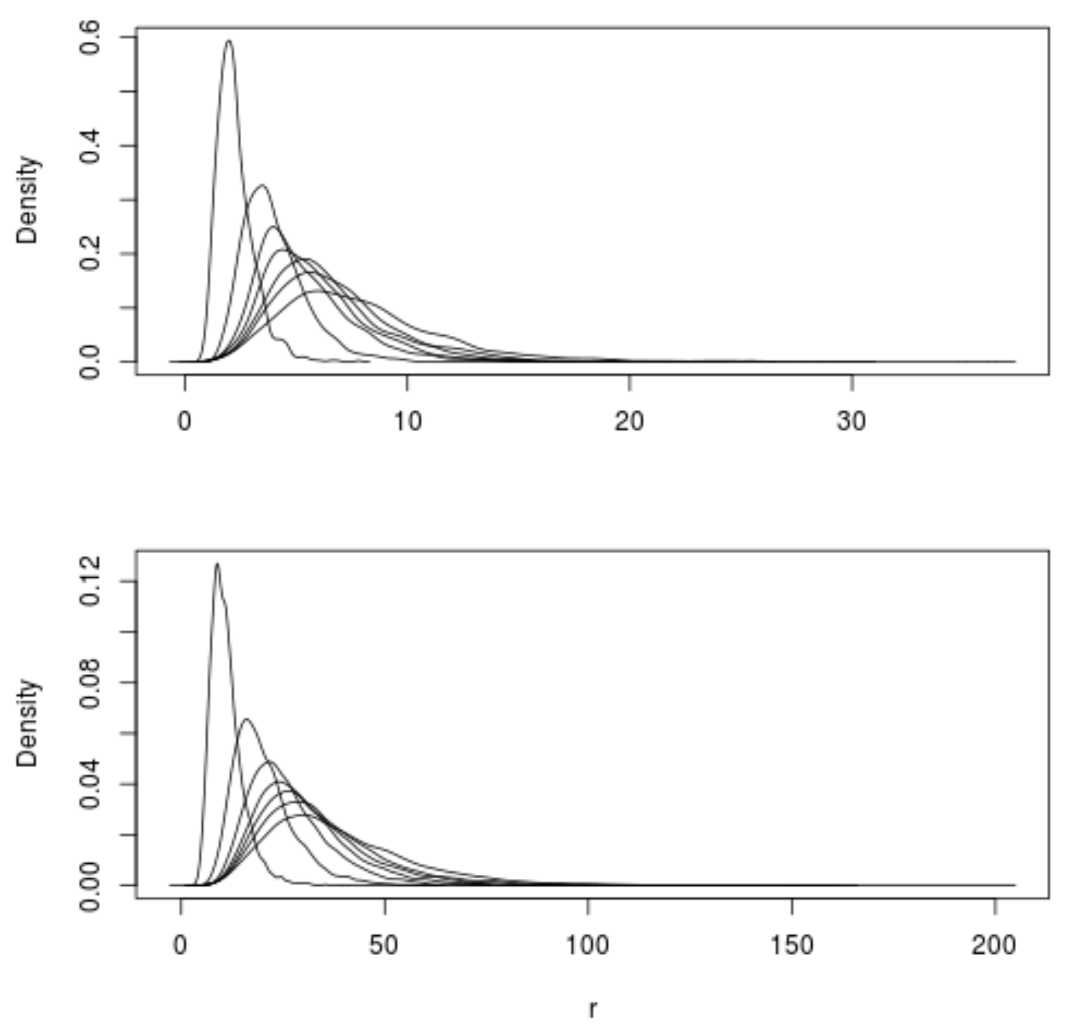
Using these assumptions, trials were generated for each and combination, where and , when and . A kernel estimator of the probability density function (pdf) for the overall system rate associated with each combination is shown in Figure 3. Observe from Equation (20) that since this figure is generated using , the horizontal axes of this figure can be interpreted as the ratio . Thus, multiplying each pdf by yields the pdf for the associated .
Inspection of Figure 3 quantifies-for a system comprised of a fixed number of basis processes and a fixed processing rate-the intuitively pleasing facts that: (i) for a fixed value, the peak value of the pdf increases, the value of the peak of the pdf effectively remains fixed, and the width of the pdf narrows as the mean process weight λ increases (i.e., the probability that the value of the overall system rate will be within a small fixed interval about the peak value increases with increasing mean process weight); and (ii) for a fixed mean process weight, the peak value of the pdf for increases and the width of the pdf broadens as increases in value (i.e., the overall peak system rate increases and the probability that will be within a small interval about the peak rate decreases with increasing system “speedup” or parallelism).
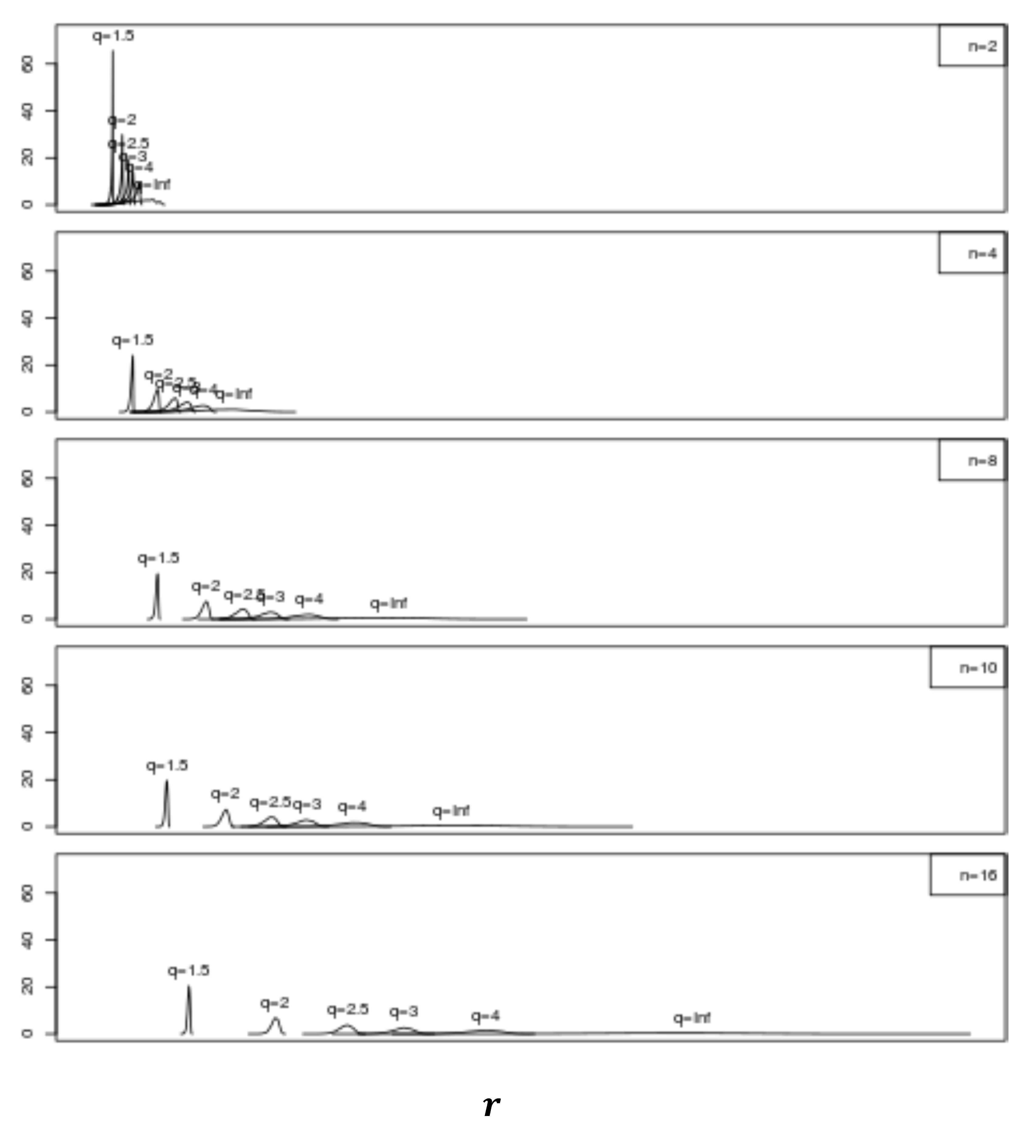
Kernel estimator pdfs were also obtained for using trials and Equation (20) with for and . The weights for each trial were determined from a Poisson distribution with . These results are presented in Figure 4 where-as expected from the Figure 3 results-it is seen for each that the peak value increases, the distribution broadens, and the value of the pdf peak decreases with increasing . Also expected is the fact that-although the pdf peak values and distribution width effectively remain the same-the distributions shift to larger values with increasing as increases.
8.2. Random Rates and Random Weights
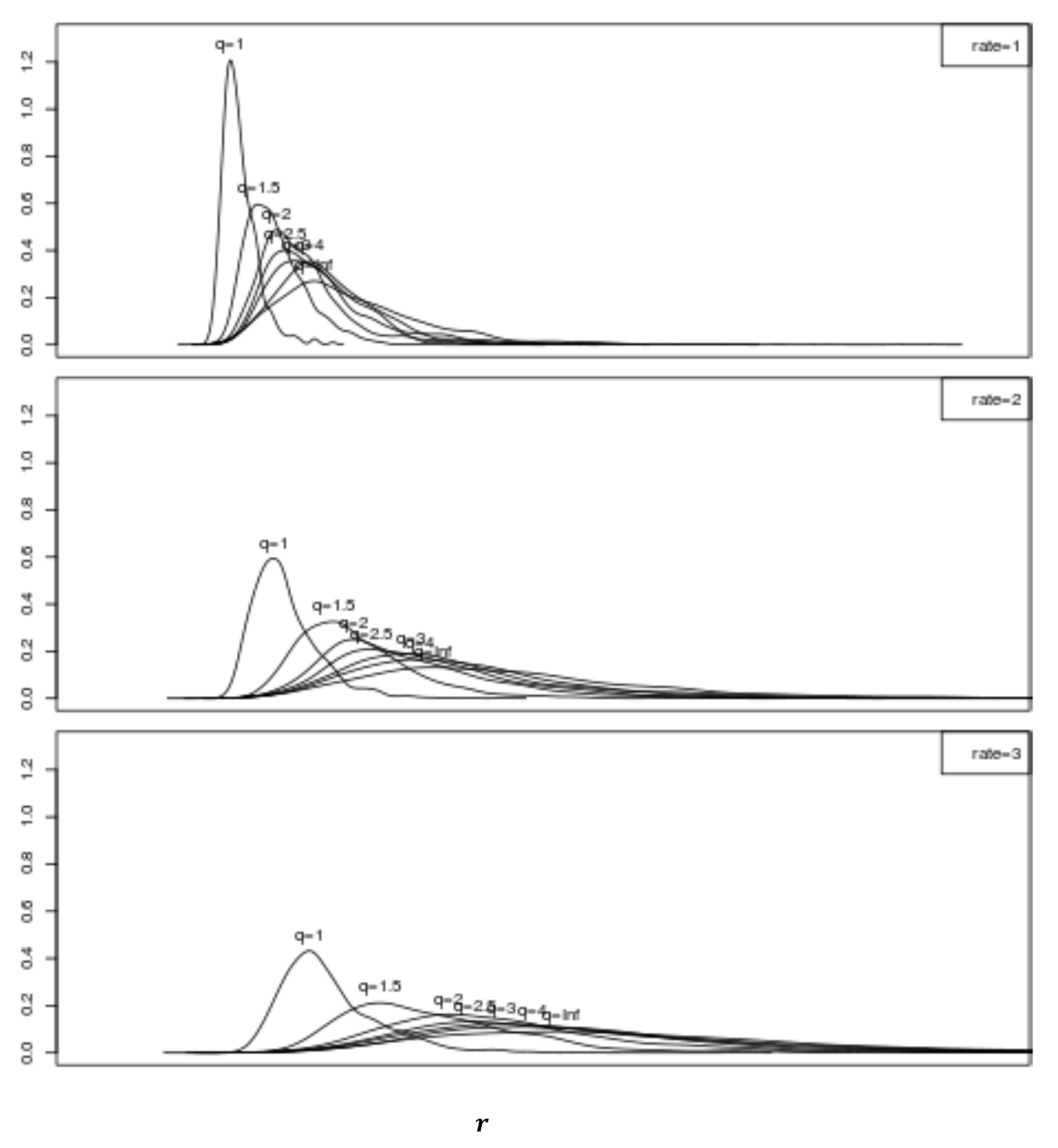
Now consider trials where for each trial—in addition to having Poisson distributed random weights as just described—the rates in Equation (15) are also randomly assigned using the exponential distribution:
Using this methodology, kernel estimator pdfs for were obtained using trials per combination for a range of values and each when and . These results are presented in Figure 5 for and in Figure 6 when is also unity and . Each of the pdfs in the two lower Figures in Figure 6 are scaled by their values, i.e., all of the resulting values are divided by their respective values, so that the pdfs for all values fit on the same horizontal axis value range.
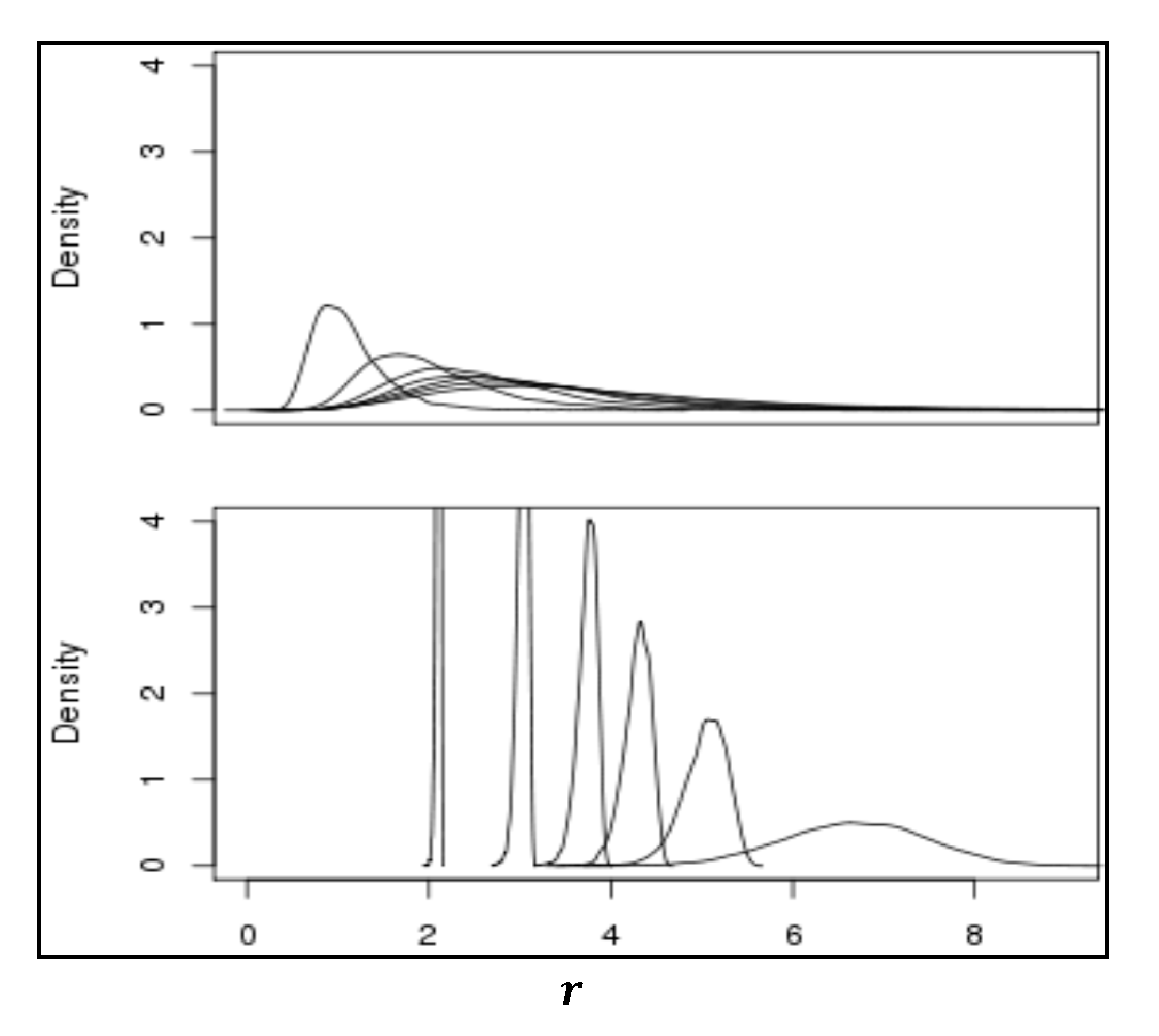
Observe from these figures that—when compared with the previous results for fixed —the inclusion of random rates causes the parameterized pdfs to be closer together and overlap. The presence of randomness increases the variance associated with each pdf and, interestingly, tends to significantly decrease the sensitivity of the pdfs to the value of . This comparison is made more clear in Figure 7 where the graphs of the pdfs for and are placed one above the other for the case where both the rates and weights are randomly selected as above when (upper Figure) and the case where the rates all have unit value and only the weights are Poisson distributed (lower Figure). Each of the pdfs in the upper Figure are scaled by the associated value.
9. Special Case Closed Form Models
Here, Theorems 17–19 are used to produce several closed form models when the performance values and the weight values are assumed to be equal for all processes in a system. Such processes are equal processes and the associated system models are special case closed form models (SCCFMs).
SCCFM 1.
If is a system such that , then , where and . The time required for the system to complete its arithmetic operations is .
Since the next model is also a direct consequence of Theorem 17 and its proof follows that of the previous model, it is stated without proof.
SCCFM 2.
If is a system such that , then , where and . The time required for the system to complete moving all of its data is .
SCCFM 3.
If is a system such that , then , where . The time delay for this system is .
Note that: (i) when , the processing is sequential and as required, the time for the systems to complete their processing is the sum of the individual times required to complete each process in the system; (ii) when , the processing time is “skewed” or “compressed” and .
SCCFM 4.
Suppose the system is comprised of equal arithmetic processes, equal data movement processes, and equal delay processes such that . Then:
where and are given by SCCFM 1 when and are given by SCCFM 2 when given by SCCFM 3 when ; and:
The time required for this system to complete its processing is:
Again, note that when , is the sum of the system delays, the time required for the system to complete processing its arithmetic operations, and the time required for the system to complete its data movement operations.
10. Applications of Special Case Closed Form Models
Special case closed form models are useful for understanding and describing fundamental properties and dynamics of CMW system performance models. The following subsections provide several examples of this.
10.1. The Effect of Upon the Dependence,
It is easily seen from SCCFM1-SCCFM3 that the differential of (with respect to ) can be written as:
Dividing both sides of this equation by yields:
which can be written as
or as
It follows from this that for these SCCFMs, varies linearly with with an associated slope of . This implies the intuitively pleasing result that for SCCFM1-SCCFM3, increasing the system’s parallelization (i.e., increasing the value) decreases the processing time -regardless of the number of basis processes that must be processed.
10.2. A Stationary Action Principle for SCCFM4 System Performance
Consider SCCFM4, assume for fixed that is time dependent, and let the function:
where , describe the system’s performance with time. Using Equation (29), it is found that:
i.e., satisfies the Euler-Lagrange equation. Consequently, is the performance Lagrangian for the system, Equation (30) is the associated equation of motion for the system’s performance, and the integral
is stationary so that its first variation vanishes (e.g., [27]). This has the following interpretation: If is the configuration space and processing begins at and is completed at , then the actual processing path followed by in during the fixed processing interval is such that:
with respect to all path variations in , which vanish at the end-points of the interval.
10.3. Invariance of the Equation of Motion
Note that for any arbitrary (twice differentiable) function , the transformed performance Lagrangian
also describes the processing path followed by in during the fixed processing interval since:
Thus, although the performance Lagrangian is not unique, by extension, it can be concluded that the equation of motion for the system’s performance is invariant under all transformations of the performance Lagrangian of the form given by Equation (33).
11. Concluding Remarks
This paper has presented a category theoretic reformulation of the Müller-Wichards system performance model. The use of category theoretic terminology provides a precise and efficient mathematical vocabulary for defining categories of systems, system performance, and system performance functors. These functors were shown to be useful for discussing factorizing systems without changing their performance and identifying model symmetries and invariants. Such formal mathematical properties of models tend to characterize aspects of the real systems that the models represent.
A practical feature of the model is that it can be implemented in a relatively straightforward manner as a software package. A user can assign to each basis process—via a gauge map—its numerical triple in the performance category. This defines for each basis process its type (arithmetic, data movement, or delay element), rate, and weight. The associated performance functor then uses these assignments to automatically generate a final performance triple for any system (string of basis processes) in the category of systems defined by the process basis set. Several other useful features of the model include using closed form performance models to provide “quick” performance estimates, as well as to provide “sanity checks” for results obtained from software implementations of the model; generating stochastic-based performance studies by treating rates and weights as random variables (as illustrated in Section 8); and applying closed form models to abstractly characterize aspects of system performance (as illustrated in Section 10).
Future research involves defining an appropriate metric on that measures the similarity between systems; and finding an approach for classifying subsets of interest in the associated metric space such that the systems within such a class are very similar [28]. An implementation of this classification scheme in a software package, which also uses to automatically evaluate in the performance of the systems in such a class can be useful for scheduling analysis, as well as for making informed high level system engineering design trade-offs.
Author Contributions
Conceptualization, D.J.M. and A.D.P.; Methodology, A.D.P.; Software, D.J.M.; Writing-Original Draft Preparation, A.D.P.; Writing-Review & Editing, D.J.M and A.D.P.
Funding
This research was funded by a grant from the Naval Surface Warfare Center Dahlgren Division’s In-house Laboratory Independent Research program.
Conflicts of Interest
The authors declare no conflict of interest.
Appendix A
Proof of Theorem 1.
This result was proven in [1]. □
Proof of Theorem 2.
This follows directly from Lemma 1. □
Proof of Theorem 3.
Let . Case i. If , then . Since , then Case ii. If , then and . Thus, . Case iii. Cases i–ii apply when and are both in or in . Now let and . Then so that . Case iv. If , then , . Since and , then Clearly, if either or both of or are the identity element for each of these cases, then . Consequently, each is a submonoid of . □
Proof of Theorem 4.
Each of these monoids determines an associated category in the manner prescribed by Lemma 1. □
Proof of Theorem 5.
Each category is small because and are singleton sets. They are connected because and , have only one object and . □
Proof of Theorem 6.
It must be shown that any morphism is both monic and epic. First show that is monic, i.e., . Observe that is monic and assume that with .
Case i. If and , then
is monic. Similarly for .
Case ii. If and , then
is monic. Similarly for .
Case iii. If and , then and
is monic. Similarly, for .
To show that morphism is epic it must be demonstrated that . Note that is epic and observe that since is commutative, then the Case i–iii arguments above still apply so that is epic. □
Proof of Theorem 7.
Consider Let and . Then because and and are real valued. If , then it is also the case that because and and are real valued. If , then , the resulting weight is real valued, and the resulting rate is real valued so that . □
Proof of Theorem 8.
This follows directly from Lemma 1. □
Proof of Theorem 9.
is a small category because is the singleton set . is a connected category because it has only one object and . □
Proof of Theorem 10.
This is a direct consequence of the fact that is cancellative (Lemma 5). In particular, is monic and is epic. □
Proof of Theorem 11.
From Lemma 3 a homomorphism is established by extending any gauge map to a unique monoid homomorphism according to:
From Lemma 2, this homomorphism corresponds to the performance functor such that and:
Similarly, for the functors . □
Proof of Theorem 12.
Since , it is clear that is also an automorphism of in which case . The theorem follows from the well-known fact that is isomorphic to the group of permutations of the elements of set [24]. □
Proof of Theorem 13.
For every , . Thus, if , then . Because is fixed, and have the same images in and , respectively, after the application of every as they did before their application. □
Proof of Theorem 14.
The existence of a commutative triangle in means that exists in . Since for every , then also exists in for every and is a CMW invariant. That the Müller-Wichards performance functor images of are also CMW invariants follows from the facts that (i) the images of these functors are CMW invariants (Theorem 13) and (ii) all functors preserve commutative triangles. □
Proof of Theorem 15.
Let be a commutative triangle in . It follows from Theorem 10 that and are bimorphisms in which case is monic and is epic and is a factorization of . Since functors preserve commutative triangles, then is the associated commutative triangle in . It is clear that the integrity of the factorization of is maintained because . Similarly for the functors . □
Proof of Theorem 16.
If is a commutative square in , then, because is equidivisible (Lemma 5), there exists an such that (i) and , or (ii) and . These are factorizations because every morphism in is a bimorphism (Theorem 10) so that in (i) and are monic and and are epic, or in (ii) and are monic and and are epic. Because each of these factorizations corresponds to a commutative triangle in , it follows from Theorem 15 that they maintain their integrity. □
Proof of Corollary 2.
If in , then it must be the case that there is an such that and or and (Lemma 5). Since , , , and are commutative triangles in , they are preserved by in , so that and or and . The result follows from the fact that every morphism in the image of in , is a bimorphism so that and are monic and and are epic, or and are monic and and are epic. □
Proof of Corollary 3.
If is faithful, then the commutative triangle in reflects to the commutative triangle in (Lemma 4). Since every morphism in is a bimorphism (Theorem 10), then is factorizable because is monic and is epic. Since , the factorization of maintains its integrity. □
Proof of Theorem 17.
That the action of the functor on is as stated in the consequence of the theorem follows from Theorem 11 and the fact that , where or when or , respectively. The remainder of the proof is by induction. (i) For ; . Now assume that . Since , it follows that . (ii) Since each weight is real valued,
and increasing by one yields:
Now assume
Since
Then
and the theorem is proved. □
Proof of Theorem 18.
The action of the functor on as stated in the consequence of the theorem follows from Theorem 11 and the fact that . It is also clear from item 2 in Section 4 that regardless of how many triples in set are combined under , the weight of the resultant triple is . The remainder of the proof is by induction. Since
and
Now assume that:
Then
and the theorem is proved. □
Proof of Theorem 19.
Since is commutative, can be rearranged and written as where and are given by Theorem 17 when and and are given by Theorem 17 when and and is given by Theorem 18 when . Because is associative, this product can be evaluated in any order. Consider first the product . The weight resulting from this product is so that:
For the product , combining with the weight of the third triple gives a final combined weight of so that:
□
Proof of SCCFM1.
The results for and follow from Theorem 17 since and . The processing time follows from the ratio . □
Proof of SCCFM3.
The results for the weight and follows from Theorem 18. In particular, the weight is because is a delay process and . The delay time follows from the ratio . □
Proof of SCCFM4.
Substituting the results from SCCFM 1—SCCFM 3 into the of Theorem 19 gives the desired result for . The time to complete processing is obtained by substituting this into the ratio , simplifying the resulting expression, and identifying the terms in the sum with processing times for SCCFM 1–SCCFM 3. □
References
- Müller-Wichards, D. Performance estimates for applications: An algebraic framework. Parallel Comput. 1988, 9, 77–106. [Google Scholar] [CrossRef]
- Döring, A.; Isham, C.J. A topos foundation for theories of physics: I. Formal languages for physics. J. Math. Phys. 2008, 49, 053515. [Google Scholar] [CrossRef] [Green Version]
- Döring, A.; Isham, C.J. A topos foundation for theories of physics: II. Daseinisation and the liberation of quantum theory. J. Math. Phys. 2008, 49, 053516. [Google Scholar] [CrossRef] [Green Version]
- Döring, A.; Isham, C.J. A topos foundation for theories of physics: III. The representation of physical theories with arrows . J. Math. Phys. 2008, 49, 053517. [Google Scholar] [CrossRef]
- Döring, A.; Isham, C. A topos foundation for theories of physics: IV. Categories of systems. J. Math. Phys. 2008, 49, 053518. [Google Scholar] [CrossRef] [Green Version]
- Wiels, V.; Easterbrook, S. Management of evolving specifications using category theory. In Proceedings of the 13th IEEE International Conference on Automated Systems Engineering, Honolulu, HI, USA, 13–16 October 1998; pp. 12–21. [Google Scholar]
- Gebreyohannes, S.; Edmonson, W.; Esterline, A. Formalization of the Responsive and Formal Design Process using Category Theory. In Proceedings of the 2018 Annual IEEE International Systems Conference (SysCon), Vancouver, BC, Canada, 23–26 April 2018; pp. 1–8. [Google Scholar]
- Kokar, M.; Tomasik, J.; Weyman, J. Data vs. Decision Fusion in the Category Theory Framework. In Proceedings of the 4th International Conference on Information Fusion, Montreal, QC, Canada, 7–10 August 2001. [Google Scholar]
- Barr, M.; Wells, C. Category Theory for Computing Science; Prentice Hall: New York, NY, USA, 2002; ISBN 0-13-120486-6. [Google Scholar]
- Pavlovic, D. Tracing the man in the middle of monoidal categories. arXiv, 2012; arXiv:1203.6324. [Google Scholar]
- Andrian, J.; Kamhoua, C.; Kiat, K.; Njilla, L. Cyber Threat Information Sharing: A Category-Theoretic Approach. In Proceedings of the 2017 Third International Conference on Mobile and Secure Services (MobiSecServ), Miami Beach, FL, USA, 11–12 February 2017; pp. 1–5. [Google Scholar]
- Mabrok, M.; Ryan, M. Category Theory as a Formal Mathematical Foundation for Model-Based Systems Engineering. Appl. Math. Inf. Sci. 2017, 11, 43–51. [Google Scholar] [CrossRef]
- Wisnesky, R.; Breiner, S.; Jones, A.; Spivak, D.; Subrahmanian, E. Using Category Theory to Facilitate Multiple Manufacturing Service Database Integration. J. Comput. Inf. Sci. Eng. 2017, 17, 021011. [Google Scholar] [CrossRef]
- Rudskiy, I. Categorical Description of Plant Morphogenesis. arXiv, 2017; arXiv:1702.04627v1. [Google Scholar]
- Haruna, T.; Gunji, Y.-P. Duality between decomposition and gluing: A theoretical biology via adjoint functors. Biosystems 2007, 90, 716–727. [Google Scholar] [CrossRef] [PubMed]
- Haruna, T.; Gunji, Y.-P. An Algebraic Description of Development of Hierarchy. Int. J. Comp. Anti. Sys. 2008, 20, 131–143. [Google Scholar]
- Haruna, T. An application of category theory to the study of complex networks. Int. J. Comp. Anti. Sys. 2011, 23, 146–157. [Google Scholar]
- Ormandjieva, O.; Bentahar, J.; Huang, J.; Kuang, H. Modelling multi-agent systems with category theory. Procedia Comput. Sci. 2015, 52, 538–545. [Google Scholar] [CrossRef]
- Zhu, M.; Grogono, P.; Ormandjieva, O. Using Category Theory to Verify Implementation against Design in Concurrent Systems. Procedia Comput. Sci. 2015, 52, 530–537. [Google Scholar] [CrossRef]
- Ellerman, D. Adjoints and emergence: Applications to a new theory of adjoint functors. Axiomathes 2007, 17, 19–39. [Google Scholar] [CrossRef]
- Phillips, S. A General (Category Theory) Principle for General Intelligence: Duality (Adjointness). In Artificial General Intelligence, Proceedings of the 10th International Conference (AGI 2017), Melbourne, Australia, 15–18 August 2017; Everitt, T., Goertzel, B., Potapov, A., Eds.; Springer: Cham, Switzerland, 2017. [Google Scholar] [CrossRef]
- Blyth, T. Categories; Longman: London, UK, 1986; ISBN 0-582-98804-7. [Google Scholar]
- Bradley, T.-D. What Is Applied Category Theory? arXiv, 2018; arXiv:1809.05923v1. [Google Scholar]
- Clifford, A.; Preston, G. The Algebraic Theory of Semigroups; Library of Congress Catalogue Number: 61-15686; American Mathematical Society: Providence, RI, USA, 1961. [Google Scholar]
- Goldblatt, R. Topoi: The Categorical Analysis of Logic; Dover Publications Inc.: Mineola, NY, USA, 2006; ISBN 13: 978-0-486-45026-1. [Google Scholar]
- Rosen, J. Symmetry Rules: How Science and Nature are Founded on Symmetry; Springer: Berlin, Germany, 2008; p. 4. ISBN 978-3-540-75972-0. [Google Scholar]
- Lanczos, C. The Variational Principles of Mechanics; Dover Publications Inc.: Mineola, NY, USA, 1986; ISBN 0-486-65067-7. [Google Scholar]
- Parks, A.; Naval Surface Warfare Center, Dahlgren Division, Dahlgren, VA, USA. Personal communication, 2017.
Figure 1.
The commutative triangle for in C.

Figure 2.
The preserved image of Figure 1 under in D.
Figure 2.
The preserved image of Figure 1 under in D.

Figure 3.
Probability density functions for for various values when and (top to bottom).

Figure 4.
Probability density functions for when , and

Figure 5.
Probability density functions for when (bottom) and (left to right).

Figure 6.
Probability density functions for when and . Each value for has been divided by the associated value of .
Figure 6.
Probability density functions for when and . Each value for has been divided by the associated value of .

Figure 7.
Probability density functions for when .

© 2019 by the authors. Licensee MDPI, Basel, Switzerland. This article is an open access article distributed under the terms and conditions of the Creative Commons Attribution (CC BY) license (http://creativecommons.org/licenses/by/4.0/).
Share and Cite
MDPI and ACS Style
Parks, A.D.; Marchette, D.J. Categorification of the Müller-Wichards System Performance Estimation Model: Model Symmetries, Invariants, and Closed Forms. Systems 2019, 7, 6. https://0-doi-org.brum.beds.ac.uk/10.3390/systems7010006
AMA Style
Parks AD, Marchette DJ. Categorification of the Müller-Wichards System Performance Estimation Model: Model Symmetries, Invariants, and Closed Forms. Systems. 2019; 7(1):6. https://0-doi-org.brum.beds.ac.uk/10.3390/systems7010006
Chicago/Turabian StyleParks, Allen D., and David J. Marchette. 2019. "Categorification of the Müller-Wichards System Performance Estimation Model: Model Symmetries, Invariants, and Closed Forms" Systems 7, no. 1: 6. https://0-doi-org.brum.beds.ac.uk/10.3390/systems7010006
Note that from the first issue of 2016, this journal uses article numbers instead of page numbers. See further details here.