Article

Complexity Economics in a Time of Crisis: Heterogeneous Agents, Interconnections, and Contagion

1
Complex Systems Research Group, Faculty of Engineering, The University of Sydney, Camperdown 2006, Australia
2
Independent Researcher, Sydney 201101, Australia
3
School of Project Management, Faculty of Engineering, The University of Sydney, Camperdown 2006, Australia
*
Author to whom correspondence should be addressed.
Submission received: 14 July 2021 / Revised: 17 September 2021 / Accepted: 9 October 2021 / Published: 15 October 2021

Abstract

:
In this article, we consider a variety of different mechanisms through which crises such as COVID-19 can propagate from the micro-economic behaviour of individual agents through to an economy’s aggregate dynamics and subsequently spill over into the global economy. Our central theme is one of changes in the behaviour of heterogeneous agents, agents who differ in terms of some measure of size, wealth, connectivity, or behaviour, in different parts of an economy. These are illustrated through a variety of case studies, from individuals and households with budgetary constraints, to financial markets, to companies composed of thousands of small projects, to companies that implement single multi-billion dollar projects. In each case, we emphasise the role of data or theoretical models and place them in the context of measuring their inter-connectivity and emergent dynamics. Some of these are simple models that need to be ‘dressed’ in socio-economic data to be used for policy-making, and we give an example of how to do this with housing markets, while others are more similar to archaeological evidence; they provide hints about the bigger picture but have yet to be unified with other results. The result is only an outline of what is possible but it shows that we are drawing closer to an integrated set of concepts, principles, and models. In the final section, we emphasise the potential as well as the limitations and what the future of these methods hold for economics.

1. Introduction

1.1. The Economics of Heterogeneity and Interconnections

Crises that disturb the economic status quo have a ripple effect that can reverberate through markets and economies around the world. The effect a crisis has on any individual entity depends on the characteristics of the entity and the nature of its connections with the rest of the economy, and this is one of the areas that complexity economics (CE) has been able to contribute to [1]. CE has its origins at the Santa Fe Institute in the mid-1980s when economists, computer scientists, and physicists came together to foster an interdisciplinary approach to addressing economic problems. Since then, a number of groups and institutions have sprung up around the world such as Oxford University’s Institute for New Economic Thinking (INET) headed by J-D Farmer, Harvard’s Atlas of Economic Complexity (AEC1 [2]), and MIT’s Observatory of Economic Complexity (OEC2), these having developed through the work of Hausmann, Hidalgo and colleagues [3,4]. Recently, some central banks, such as the Bank of England [5] and the Canadian Central Bank [6], have begun to explore CE methods, such as agent-based models (ABMs), for policy-making and in their approaches to modelling market dynamics. This is an approach that has been growing in its sophistication and accuracy with a paper by Poledna and colleagues [7] having recently won 1st prize in the Complexity and Macroeconomics Competition held by Rebuilding Macroeconomics for producing an ABM that is comparable in forecasting ability to traditional DSGE (Dynamic Stochastic General Equilibrium) models.
CE has sometimes been critiqued for not being a single theory or a unified approach to economics [8]. This is in part because in practice it is an ecology of ideas, analogies, and methods combined with large amounts of domain-specific data that are used to address particular problems, freely borrowing from other fields in order to do so. However, this also belies a technical consistency in the approach CE adopts. In particular it focuses on the formal strengths of models that have often been validated in other fields and then applies the appropriate economic framework around the analysis, thus allowing models to develop independently of both economic ideology and the other fields that inspired the initial analogies. For example, ‘spin models’ [9,10], binary state models that represent agents as, for example, buyers and sellers, have been used extensively as simple models by CE theorists to develop their intuition for the micro-economic agent-to-agent interactions that result in the emergence of nonlinear macro-economic dynamics. The phase transitions we see in spin models then help frame our thinking of the non-linearities of complex market behaviour such as the two-phase dynamics discovered by Plerou et al. [11]. This has also been used extensively in the work of Brock and Durlauf [12] and Aoki [13], for example, in understanding the interactions between agents and the emergence of multiple equilibrium.
These models first appeared in the field of physics which remains a significant source of inspiration for CE [14,15], as does the mathematics of network theory [10,16] and evolution [17,18], ideas that have been brought together in work on evolutionary game theory on networks in order to understand the emergence of cooperation [19] and spreading dynamics over networks [20]. On the topic of evolution in economics, Brian Arthur, who coined the termed ‘complexity economics’, has written [21]: … because complexity economics looks at how structures form or solutions come to be ‘selected’, it connects robustly with the dynamics of evolutionary economics. Evolutionary economics also explicitly accounts for the path dependencies of outcomes and the heterogeneity of agents, as Volmir writes in his review [22] of Nelson et al’s book [23]:
… technological trajectories are a cumulative process of searching for “new ways to do things”, providing the reader with a framework to explain emerging behaviors such as lock-ins, ‘anti-commons’ problems… Since the 1960s, innovations began to be viewed as multi-interactive phenomenon, which entails a cumulative process between different agents and institutions, a fact ignored by standard economics… Once the cumulative process is understood, it is impossible to deny that there are differences in the ability of distinct firms to accumulate knowledge.
This combination of heterogeneity, path dependency, interactivity, and innovation are all hallmarks of the ‘world view’ of CE.
With these concepts in mind, theory and empirical study in economics have been moving into an era of networks and heterogeneous agents, and along with this progression comes a growing awareness of the systemic risks of a highly connected society. Take, for example, the network of international trade relations that have been a lynch pin of modern trade development recently reviewed by Carrère et al. [24]. In this domain, a central model has been the gravity model of trade [25], and in its simplest form is conceptualised similarly to that of gravity in physics. In physics, the attractive forces F between two objects of masses M 1 and M 2 is proportional to the product of their masses divided by the square of the radial distance r 2 between them:
F = G M 1 M 2 r 2
where G is the universal gravitational constant. The gravity model of international trade has a very similar form where the trade flow T i , j between two economies with gross domestic products of P i and P j and the geographical, political, social, or some other measure of separation is represented by D i , j , is expressed by the relation
T i , j = C P i P j D i , j
where C is a constant of trade. See Anderson [26] for the theoretical foundations and extensions. This formulation, first framed in 1954 [25], lends itself naturally to a network analysis in which each T i , j = T j , i is the symmetrical weighted link in a network connecting nodes of size P i and P j . For a fixed distance, as the sizes of the economies grow the flow of trade between them increases, but if the distances between these same economies were increased the trade flows would decrease in inverse proportion. The analysis of these networks has been further extended to the micro-economic level through the work of Bergstrand [27], for example, providing a much more granular conceptualisation of trade in which the gravity model is a reduced form of a more sophisticated partial equilibrium model of trade.
The network model of trade is more general than the gravity model though. For example, Rauch has studied the social networks of trade [28] and the relationships between networks and markets [29]. In a similar study, Chaney [30] looked at the network structure of trade where firms can only export into markets in which they have contact and acquire new contacts both at random as well as through their network of existing contacts, thereby introducing an element of randomness to network formation. The specific varieties of what is traded over these networks have also been considered in some detail, with Dalin et al. [31] looking at the trade in ‘virtual water’, the amount of water needed to produce food, and the global trade in arms studied by Arkerman and Seim [32]. Alongside this appreciation of the role of network topology and flows of trade is a further appreciation of the heterogeneity of the nodes themselves, i.e., the highly varied characteristics of the countries, companies, and individuals that are the linked agents.
The recent growth of research in this area has been stimulated, at least in part, by the growth in international trade and the use of Free Trade Agreements between a large number of economies and consequently a need to better understand how this has shifted regional economies. This is because although there had been no global free trade agreements since 1994 [33], whereas the number of regional or bilateral trade agreements between countries (e.g., NAFTA, EU, and APEC) grew from 50 in 1990 to more than 280 in 2017 [34]. This has led to a deeper interest in systemic risks such as the fragility of supply chains [35], the interaction between trade networks, trade wars, and firm value [36], as well as trade related climate change [37]. However, this has been in parallel with an enormous growth in the study of ‘complex systems’ through the lens of network analysis, a field in which recent research began with Watts and Strogatz in 1998 [38] and Barabási et al. in 1999 [39], and it has played a core role in many fields over the last twenty years. This has particularly been the case in economic research where the formal methods of network science have been used by non-economists, often but not always physicists, to study the abstract properties of trade networks [40,41,42]. While the recent connection between physics models and economic data has not always been a harmonious one, it has been productive in certain fields of economics with several articles by prominent researchers on both sides of the debate having voiced strong opinions on the success or otherwise of these methods [43,44,45].
These debates have been had at the macro-economic level as well as at the market and micro-economic levels, all of which has been a part of a steady revolution in economic thinking over the last 30 years. Some of the earliest work using simulations or a ‘complex systems’ approach [46] includes the work of Brian Arthur and colleagues on the simulation of financial markets [47] and other models of collective economic behaviour [48] where traditional assumptions, such as equilibrium or rational choice, are relaxed in order to study the evolutionary dynamics of markets and under what circumstances an equilibrium state might naturally come about with these assumptions relaxed [49]. Other models, such as bifurcation models in which a form of dynamic equilibrium is presumed, are suited to partial equilibrium analysis in the sense that it is the non-equilibrium transition between alternative stable states that is most interesting, see Rosser Jr.’s review of economic Catastrophe Theory for example [50].
Within the context of complexity economics, this article reviews several recent research directions at multiple different levels of analysis as well as some of the work that we have carried out in recent years. This includes our work on applied network theory [20,51,52,53,54], bifurcations and systemic risks [55,56,57,58,59,60], agent-based modelling of economic markets [61,62,63,64], the theoretical limits of ‘rationality’ and strategic choice [20,65,66,67,68,69], and how information theory can be used to understand the dynamics of these systems [70,71,72,73,74,75,76,77]. The purpose then is to place this research in the context of the work being carried out in other groups around the world. We hope that further developments of these areas will ultimately lead to larger models that can be used to better understand the macro-economic response of an economy to global shocks during a crisis such as COVID-19 or the Global Financial Crisis (GFC). In the following subsections, we introduce the central themes of this work that are the basis of the sections in the main body of this article.

1.2. The Household Level: Theory and Simulation

As we write in mid-2021 the pandemic continues to push economies around the world into lockdowns where social distancing measures are put in place, restricting our freedom of movement as well as the ability of the economy to function properly. At the level of households, the first two sections investigate if the financial distress caused by the pandemic could cause a new period of stress in economic markets such as the one observed during the GFC. This topic has two parts: the first is a stylised agent-based simulation without any real-world data, and the second is a more realistic simulation using real data from the Greater Sydney housing market. The purpose of these case studies is to illustrate the strengths and weaknesses of the two approaches as well as the relationship between them.
In Section 2, we implement the modified diffusion model with financial constraints first proposed by Gallegati et al. [78] in order to model the ‘period of financial distress’ prior to a market decline for markets in general and later used as a model of housing markets specifically [79]. At the individual agent level such a period might occur when the agent, such as a firm or a household, is faced with the not yet realised but highly probable chance of not being able to meet their financial obligations [80]. In the broader sense of a whole market this can occur because a subgroup of agents have wealth constraints that limit their ability to buy assets outright and so they need to borrow to buy assets that then, through the evolution of the market price, become undervalued and as the assets are then distressed some over-leveraged agents need to sell, pushing prices down even further than fundamentals suggest is the equilibrium price. The effect of leverage on market stability has been extensively studied in housing markets [81,82] and agent-based models of financial markets [83,84] and in the work of Kindleberger [85], periods of financial distress are a general pattern in many bubbles and their subsequent crashes throughout the last several centuries. In Kindleberger’s words [85] (p. 11):
Then an event—perhaps a change in government policy, an unexplained failure of a firm previously thought to have been successful—occurs that leads to a pause in the increase in asset prices. Soon, some of the investors who had financed most of their purchases with borrowed money become distress sellers of the real estate or the stocks because the interest payments on the money borrowed to finance their purchases are larger than the investment income on the assets. The prices of these assets decline below their purchase price and now the buyers are ‘under water’—the amount owed on the money borrowed to finance the purchase of these assets is larger than their current market value.
In Section 2, we reproduce the model of Gallegati et al. [78] to illustrate this period of financial distress.
In Section 3, we move from these theoretical considerations towards the more applied level of the Australian government’s response to the COVID-19 ‘event’, to use Kindleberger’s terminology, and its impact on the housing market. In response to the pandemic, the government moved to close borders [86] that reduced the influx of temporary residents (e.g., students and short-term workers), resulting in a decrease in the demand for rental properties and the corresponding decline of the rental prices [87] which has impacted the income of property investors. Second, decreasing the cash rate by the Reserve Bank of Australia [88] has increased the incentive for mortgage borrowing among households that are otherwise stressed due to COVID-19, which has resulted in an increased demand in housing and a corresponding increase in prices [89]. Third, the government’s ‘JobKeeper’ and ‘JobSeeker’ payment schemes [90,91] intended to support households’ individual budgets and to stimulate their consumption activity created an auxiliary source of income for households, which has arguably altered their budgeting incentives.
These government policy-driven macro-economic factors have combined with the micro-economic effects of reduced spending for holidays due to travel restrictions and other changes in household behaviour such as reductions in food wastage (as reported in other countries during COVID-19 [92]) and so impacting household expenditure, the consequences of which is household savings of $100 billion during 2020 [93].3 This has had the consequential effect of increasing pressure on the housing market in 2021 as the extra savings has fuelled further interest in house buying across Australian markets. As the Australian Bureau of Statistics reported [94]:
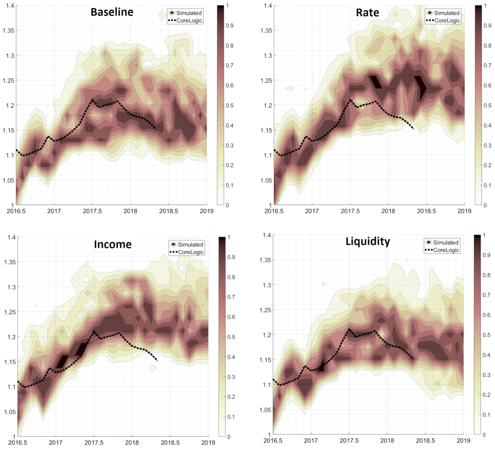
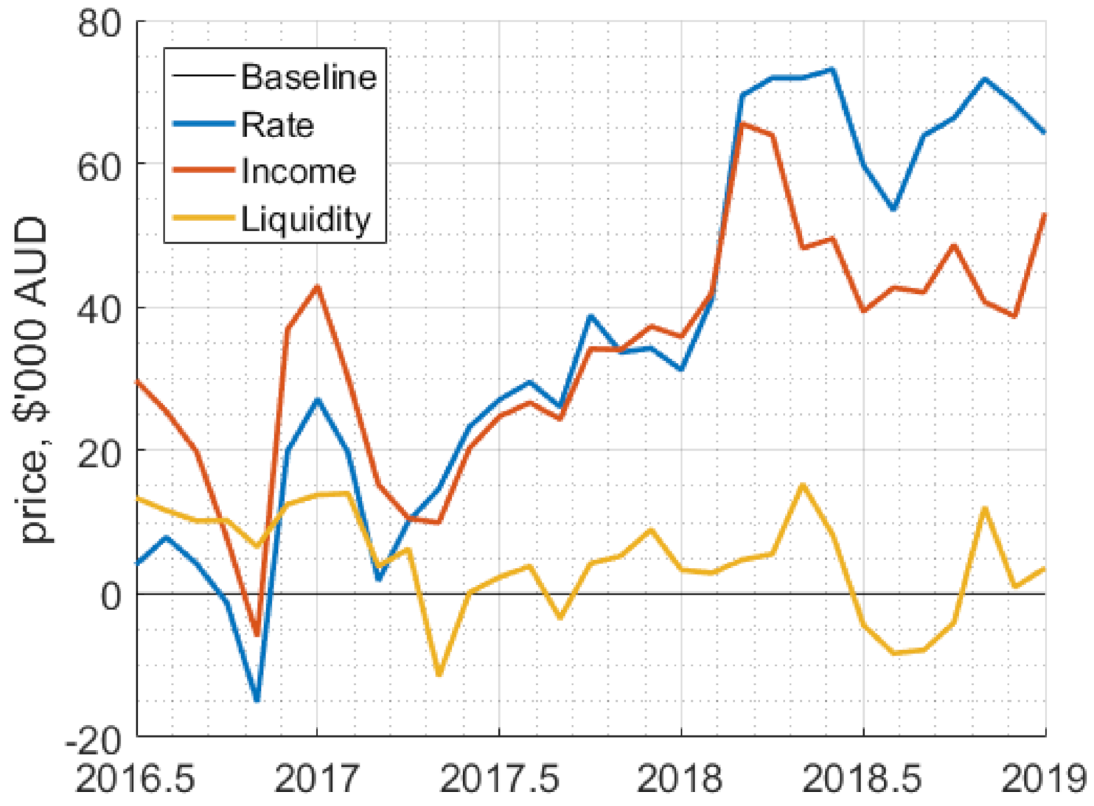
Increased housing market activity was driven by an expansive monetary policy and support through government policies such as Homebuilder and other state specific initiatives, as well as pent up demand (due to lower activity during the June quarter [2020] COVID-19 lockdown period). As auctions and open home inspections picked up in September quarter (with the easing of social distancing measures), greater demand than there was housing stock on the market saw property prices rebound
These factors have contributed to an already highly valued Australian housing market [62,63] and will likely continue to contribute to wealth and housing inequality into the future. We emphasise this combination of government policy and micro-economic factors because we want to illustrate how emergent consequences arise from changes in individual behaviours during a crisis, something that needs to be explicitly modelled because there is usually, as in the case of the GFC and COVID-19, no previous macro-economic data on which to base sound judgement, so estimates of the impact of individual behaviour need to be used, and how these behaviours drive the macro-economic dynamics that policy-makers want to manage.
With this Australian-specific perspective in mind, in Section 3 we compare the methods of Section 2 with those of a model of the Greater Sydney housing market to illustrate the strengths of a realistic model that uses high-resolution market and socio-economic data in which household constraints are varied to reflect key aspects of the COVID-19 crisis. We show that the effect of COVID-19 on Sydney house prices is the opposite to that of a bubble–crash dynamic; house prices increase significantly in the model and this has been observed in recent price movements across Sydney and other Australian capital cities, lending significant credence to the use of agent-based models to simulate out-of-sample dynamics during a crisis.

1.3. Financial Markets and Systemic Risks

Financial market crises are a common topic of study for researchers outside of mainstream economics. This is due in part to the extensive amount of data available which allows financial markets to be analysed very well with the tools of computer science and physics that were initially developed for studying large stochastic systems with interacting elements. Some of the earliest work in this area that continues to drive research is in the study of the so-called stylised facts of financial markets, such as fat tails and clustered volatility [95]. One of the earliest debates was over the best model to use for market fluctuations: cascading turbulence or a truncated Lévy flight [14,15,96,97]. This led to a long and fruitful series of investigations into the dynamics of the univariate time series of financial market indices [98,99,100,101], with recent contributions from our group in this area as well [102,103,104,105].
At a more granular level, the analysis of markets can be seen as an interaction between prices that, to at least some extent, contribute to the (co-)movement of other prices, inducing a dynamical asset network that can be studied for its stability properties. This type of analysis can, for example, extract market sectors from price movements by examining the largest eigenvalues of the market’s cross-correlation matrix [106] as well as using random matrix theory to distinguish between random and non-random correlations [107], methods that were originally motivated by models in physics. As an approach to understanding crises, such as the Black Monday crash of 1987, and optimal portfolio selection, Onella and colleagues applied correlation-based network analyses in order to understand market risks [108,109,110,111]. Our group has extended these methods to information theoretical methods in order to study the nonlinear properties of markets and other types of nonlinear dynamics [52,55,70,112]. Extending these methods by using information transfers between equities such as Granger causality [113] or transfer entropy [71,114] results in fundamentally different networks of relationships between equities [70] and consequently different risk profiles depending on the different measures of relationship used.
In order to study some recent market events that have been particularly turbulent and have yet to be studied in detail, in Section 4 we use transfer entropy (see, for example, in [70] and [Chapter 6] in [71]) to infer a temporal flow of information between equities during the periods covering three market events: the US Federal bail out decision of 2008, the Flash Crash of May 2010, and the COVID-19 crash of 2020, together with three other random control dates. For each of these events, we use tick-by-tick financial data that allow us to study the day before the event, the day of the event, and the day after the event with three thirty-minute periods used to compute transfer entropy of the Dow Jones Index. This gives us considerable fine grained insight into the micro-evolution of information flows through the market and their relationship to overall market dynamics.

1.4. Trade Networks: Internal and External Trade in Value Added

As mentioned in the first section above, trade networks are vital to the economic development and prosperity of a country’s economy. Since the earlier work on gravity models, work has developed extensively in understanding the relationship between trade within a country’s economy and trade between different economies. Developments such as the Observatory of Economic Complexity [115] (https://oec.world, accessed on 13 October 2021) have taken significant amounts of trade data and converted it into country-specific trade network analyses that can be drilled down into the sub-market sectors as well as, in many instances, the distinct economic regions within a country. Research stemming from this work has established important links between these trade networks and the specifics of income inequality [116], the environment [117], and employment [118], all issues that are of central concern to the sustainable growth and development of a country.
These networks have developed much more slowly over time than other networked aspects of the economy such as financial markets or housing markets, and their disruption and subsequent recovery might also be expected to be somewhat slower. However, even short-term shocks to trade networks can have a significant and long-lasting impact on trade links such as agri-food trade networks [119,120] and other commodities [121,122] that are heavily traded as physical goods across the globe. These have been studied in detail for previous crises, for example the role of the inter-bank network of debt during the GFC [123]. In Section 5, we look at the intra- and inter-economic trade data beginning at the industry sector level to examine patterns in the trade of goods and services between market sectors. In working to understand the long-term shocks caused by COVID-19, we can use analyses of this type to form a better picture of the complexity and interrelationships of sub-market trading and its implications of policies.

1.5. Business Sector Analysis

In Section 6, we discuss the impact of global crises on businesses through the lens of projects and their role as vehicles for economic transformation. At an operational level, projects are a useful framework within which organisations can plan and control the delivery of products and services that generate income or otherwise benefit businesses and their customers [124]. As is the case for other elements of economic development, the effect that a crisis has on businesses or individual projects depends on their individual characteristics and the nature of their connections with the rest of the economy. Large projects and large portfolios of related smaller projects can have an out-sized impact on economic development and their stalling or failure during a crisis has a consequential knock-on effect for the rest of the economy. Using data reported during the COVID-19 pandemic, we show how projects are strongly connected with, and have been impacted by, their respective economies, with a significant number of projects being cancelled or suspended.
In particular, we look to a class of projects known as ‘megaprojects’ that are commonly used to deliver very large, complex, and costly outputs such as infrastructure, water, energy, and mining ventures [125,126,127]. Their extreme scale is reflective of the functional complexity of megaprojects which are themselves often initiated to facilitate the productive efficiency and delivery of many other goods and services. In other words, large, complex projects are often singular economic exercises around which other economic developments organise themselves, providing support to downstream development projects in multiple industrial sectors.
This is most apparent in multi-billion dollar projects such as energy or road projects that facilitate further development throughout the economy. For example, Olds [128] has examined urban mega-projects on the Pacific rim (Vancouver, Yokohama, and Shanghai) and the relationship between local economic development and globalisation. Similarly, Zekovic et al. [129] has looked at megaprojects in the context of urban planning and development. Most telling of all though is the enormous amount of infrastructure that is required to support GDP growth in the coming decades and the role of megaprojects in this development. In a 2017 article, Söderlund et al. [130] wrote:
One reason for such acceleration in megaprojects can be gleaned from the projections of infrastructure to meet the world’s ever-increasing needs for economic growth and improvements. McKinsey (Garemo, Matzinger, & Palter, 2015) estimates that the world needs to spend about US$57 trillion on infrastructure by 2030 to keep up with the expected GDP growth. The Organisation for Economic Co-operation and Development (OECD) estimates that ‘global infrastructure investment needs of US$6.3 trillion per year over the period of 2016–2030 to support growth and development’, which exceeds the figure proposed by McKinsey.
Due to their extreme scale and impact, megaprojects often play a pivotal role in the shaping of an economy. However, the inverse may also be argued, i.e., where there is a disruption like that caused by a global shock such as COVID-19 this can precipitate the cancellation or pausing of megaprojects as their funding bodies reassign previously budgeted capital to other more pressing needs and the resultant loss or delay of innovation and value. The net effect is to push back the infrastructure necessary to support the economic growth of the next decade.
As some countries begin to emerge from the grip of the pandemic, there are moves to spur economic recovery by initiating large infrastructure projects. Starting (or restarting) significant numbers of projects over a short period will likely stress delivering organisations as they seek to rapidly revive projects and recover the work force at the same time as competing for newly announced infrastructure projects. This restart may create shortages of raw materials as global supply chains respond to rapidly increasing demand and competition as skilled resources, stressing already compromised global value chains such as those described in Section 5.

1.6. The Structure of the Article

In the sub-sections above, we have given a brief overview of some of the recent literature as well as a review of the tools that are used in what follows in this article. The progression of the sections from Section 2 through Section 5 are in approximate order of increasing degrees of coarse-graining. Section 2 is purely theoretical and every agent is completely described at the discretion of the modeller, however this level of information comes at the price of lacking in real-world precision. Section 3 is again a simulation, but it is populated with realistically calibrated agents and an economic context that is based on the real world while also being expected to faithfully reproduce empirical observations of market behaviour. Section 4 has no explicit agents or models of interactions, instead it empirically examines the interactions between agents that can be inferred using multi-variate time series from financial markets. Section 5 looks at an even further aggregated level, starting from data of entire industry sectors and looking at the trade in value added between sectors within an economy as well as between economies. Although each of these layers interact with each other to produce multiply layered networks of interactions, we do not yet integrate them in a unified model; this is left for further development and is an open research effort in this field. Finally, in Section 6, we discuss the unique aspects of project economics and their role in development, both during and post an economic crisis.
Each section should be seen as a distinct and relatively independent case study that illustrates methodologies or principles in action, without going into a great deal of detail (references are provided to work describing the relevant details). In particular, we have used the methods described above to illustrate various strengths and weaknesses of particular ideas from CE applied to the analysis of an economy, usually with an Australian perspective for concreteness. This is not intended to be a complete analysis of an economy, for example, we have omitted central banks, commercial banks, and other key institutions and markets. Nor should these be seen as an integrated approach to modelling an economy because we have yet to make clear the connections between the different elements we will describe. Instead, the intention is to illustrate the multiple directions of research that are being pursued and that are now being drawn together to contribute to a unified “whole of system” approach to modelling large scale economic phenomena. In the meantime, it is hoped that this article gives some insight into what is presently being developed and what the future holds for the field.

2. Periods of Financial Distress in an Agent Based Model

As mentioned in Section 1, in the work of Kindleberger [85] the initial cause of financial distress can be the action of a few agents that by some means come to believe that they are in stress or a bubble and that, once they have acted on this belief, the rest of the market comes to a similar realisation and that many of them may need to sell in order to manage their financial position. What initiates a market sell-off is a matter of ongoing debate so to make our ideas concrete in the form of a relevant simulation we follow the work of Gallegati et al. [78] in order to simulate an endogenous market crises. The purpose in using this model is that it includes agent level (household) financial constraints as a primary contributor to an asset market crisis, where the asset might be equities, houses, or something else. These constraints are related to the costs of buying and selling the asset, which are implicitly relative to the total household budget, if either the household budget changes or the transaction costs change for a large enough portion of the market then a market-wide period of financial distress may result, and it is these shifting household constraints that we will relate to the COVID-19 crisis in Section 3.

2.1. The Theoretical Framework

In [78], there is a population of buyers and sellers facing a binary choice problem for a single risky asset. The simulation runs for a number of steps indexed by t and at each step an agent i chooses a strategy w i , t { 1 , 1 } where 1 represents selling and + 1 represents buying. The asset’s underlying price dynamic is given by
p t = p t 1 + k w t + σ z t
Here, the price evolution is a sequence of n + 1 values { p 0 p n } with a given p 0 , z t is a Weiner process (noise), and σ is the strength of the noise. Excess demand is the average of all agents’ choices at time t where the mean strategy is w t = w i t and therefore k w t is the k-weighted influence that excess demand has on price (set to k = 0.4 in the original paper). The expected excess demand at t is assumed to be w t e = w t 1 . The utility for each agent i is given by
U i t = ( p ¯ t p t 1 ) w i t + J w i t w t e + ϵ i t
in which p ¯ t is a single stochastic adaptive learning process for all agents:
p ¯ t = p ¯ t 1 ρ ( p ¯ t p t ) + σ 1 z 1 , t
and ρ [ 0 , 1 ] controls the adaptation speed. The strength of the agents’ interaction with one another is controlled by the parameter J, as it is through the J w i t w t e term that individual choices are connected to all other choices via a mean market estimate of excess demand. The agents make their decisions based on the expected benefit of trading using both the recent observable price changes and the relative excess demand weighted by a herding factor (see Equation (4)). The decision-making process each agent uses is based on a value function V i , t :
V i , t = U i t if W i , t 1 > θ W i , 0 if W i , t 1 θ W i , 0
where W i , t is the wealth of agent i at time t, W i , 0 is the initial wealth of each agent and θ is some real valued proportion of the initial wealth such that, if the wealth falls below a threshold value of an agent’s initial wealth then they will not trade. Then, a choice w i t { 1 , 1 } is made according to the probability:
P ( w i t ) = P ( V i t ( w i t ) > V i t ( w i t ) )
This trading model follows the social interaction approach of Brock and Durlauf [12]. The full simulation can be summarized as carrying out the following steps for a total number of T iterations:
  • Compute agent’s decisions w i t using Equations (4), (6), and (7),
  • Asset prices are updated using Equation (3),
  • Agents realize profit/losses and update their wealth,
  • Agents compute a new expected price.
For a complete description and background of the algorithm see the original paper [78].

2.2. Simulation Results

By reproducing the original model we are able to achieve similar results to the original article, and we note the following:
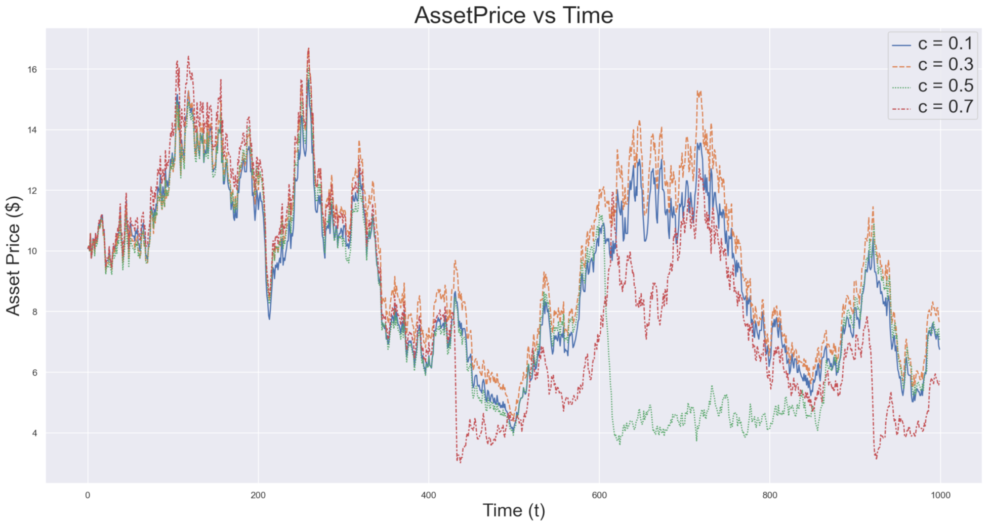
  • A bubble characterized by a PFD is produced only when transaction costs are sufficiently high, see Figure 1. In the absence of high transaction costs no crashes are observed in the simulations.
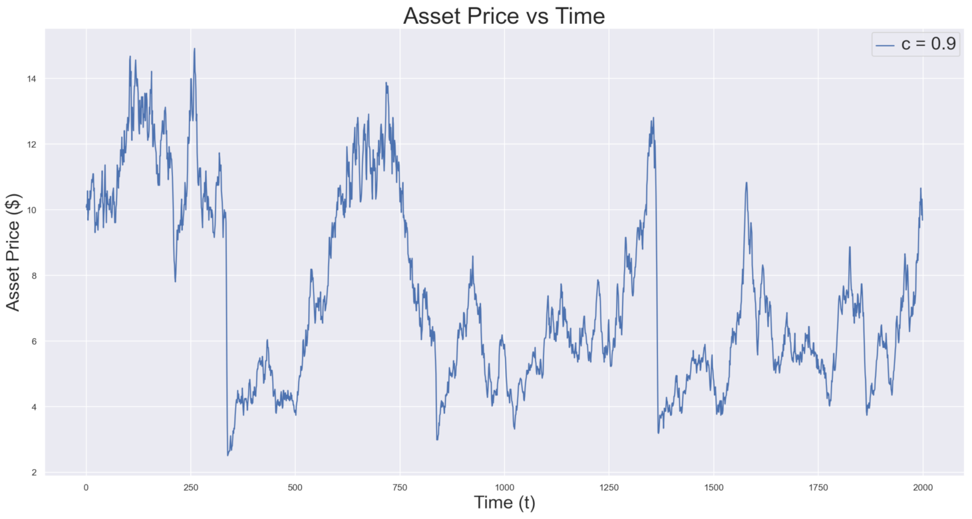
  • High financial costs cause a pattern of crashes in Figure 2. As a hypothesis for the cause of financial distress, high transaction costs have the drawback of causing repeatable patterns that are may not be realistic.
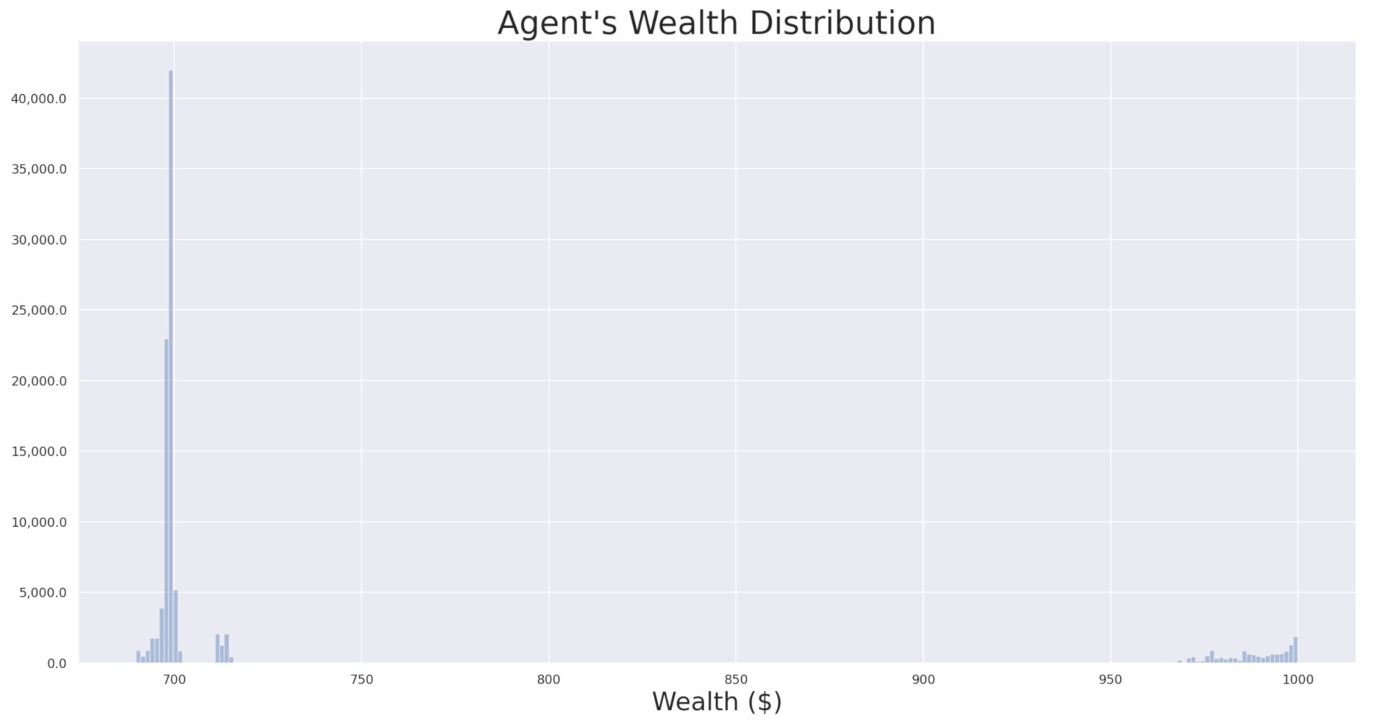
  • The evolution of the wealth and the distribution of the agents explain the bubble (Figure 3). We can see two densities of wealth that correspond to the beginning of the simulation and right before the crash. It demonstrates that financial distress seems to be correlated with the occurrence of shocks.
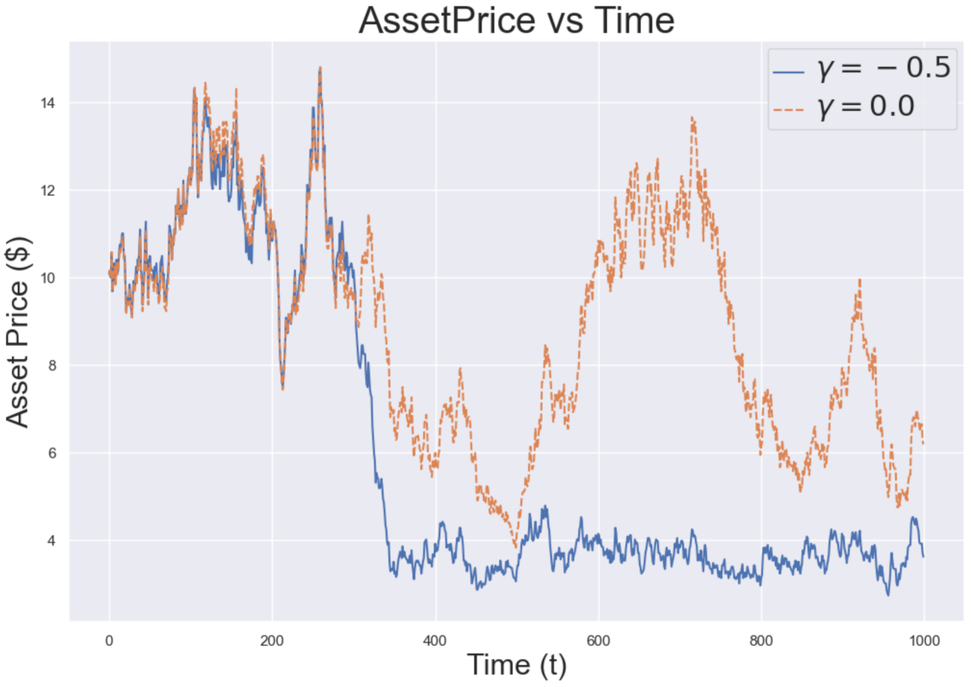
  • Changes in the herding factor, J, affect the amplitude of the bubble, making social interaction an important component of how financial contagion spreads and how the shock ultimately unfolds into a crisis.
While in this model financial distress is caused by the presence of excessive transaction costs, Gallegati et al. [78] make it clear that the use of transaction costs is only a modelling tool and many other mechanisms can produce the same result. We consider an alternative scenario with an external field factor, γ , introduced in the utility function, representing the market sentiment and we show that, similar to high transaction costs, it too can cause market shocks more serious than those that might be expected for an equivalent normal distribution. As the number of equity pairs with statistically significant TE values does change over a m
In the presence of market sentiment, the utility function evaluated by the agents becomes
U i t = ( p ¯ t p t 1 ) w i t + J w i t w t e + G + ϵ i t
where G N ( γ , 0.01 ) , which means that under normal circumstances ( γ = 0 ) the utility to buy or to sell is not affected, but under exogenous influence the agents have a higher propensity to either buy or sell. We consider a scenario in which an external event occurs at timestep t = 300 and as we can see in Figure 4 this causes a steep decline in market prices, although at a slower rate than the ones caused by financial distress.

2.3. Remarks

Agent-based models are a powerful tool to simulate the interactions between heterogeneous agents in complex economic environments and to test hypotheses about emergent behaviour originating from those interactions. In this model, Gallegati et al. extended their earlier work by the inclusion of financial constraints at the individual agent level, which endogenously induces a strong nonlinear dynamic. Such simulations are an important tool for calibrating our intuition, in terms of interactions and constraints, for the purposes of policy-making as they can be used to evaluate alternative scenarios and guide decisions that can lead to better policies. However, these are only a guide, and what is needed to extend this work to a more practical understanding of policy-relevant parameters are agent-based models that can also be used to perform more fine-grained scenario sensitivity testing using real data tuned to a specific market as we demonstrate in the next section.

3. Trading Houses: An Agent-Based Analysis of Stressed Markets

Our recent work looking at the Australian housing market [62] has shown that from 2016 onwards this market has been in a volatile state in which high housing prices have been coupled with higher than usual fluctuations in their values, an aspect of the Sydney market that is not unlike the periods of financial distress covered in Section 2. This behaviour contrasts with the previous decade (between 2006 and 2016) in which there were periods of both growth and decline, but the trend has been much less volatile. In this work, we argued that the current state of high uncertainty has been caused by a combination of two factors: the households’ trend-following aptitude, i.e., their tendency to ‘market herding’ behaviour [131,132], and their collective propensity to borrow. The former behaviour is quantified by a parameter that reflects a household’s desire to follow the price trend, as accounted by the balance of the monthly costs associated with acquiring a house and the anticipated long-term gains in house value due to market growth. The latter behaviour is quantified by either the mortgage rate or by the observed statistical relationship between a household’s income and mortgage. Using a multi-agent model that has realistic data and dynamics that are known to follow real market prices, we were able to probe the model for the mechanisms that drive this new behaviour, without changing the underlying interactions and mechanisms in the model.
It is important to realise that the higher volatility in market prices have been observed not only in the modelled market, but also in the actual market. Such uncertainty is typically an indication of a critical transition, when the system approaches a bifurcation point that separates two (or more) states with relatively stable dynamics such as that studied by Scheffer et al. [133] or the period of financial distress of Gallegati et al. As the system is composed of a large number of interacting agents, taking account of all the factors that influence the evolution of each individual agent—even in the real market—is too difficult a task, resulting in the behaviour of agents being essentially indistinguishable from a stochastic process. This individual stochasticity is compounded by the stochasticity associated with the emergent collective behaviour of a large number of agents. Such phenomena have been observed in other systems [134,135,136] in which the details of individual interactions between agents are unknown and possibly not even measurable for practical purposes, yet their collective behaviour can still be coherent overall and may provide indicators of the existence of a bifurcation point and the associated systemic risks. Our understanding of such phenomena in socio-economic systems is generally less clear than in these other systems and it is an active area of research.
Agent-based modelling provides a tractable computational tool study stochastic social systems, and housing markets are one of its feasible applications. In these models, we mimic the actions of real households subjected to market conditions (e.g., mortgage rates, housing stock, budgeting constraints, etc.). This allows us to not only identify possible causal relationships between the parameters and the observed market behaviour (e.g., price or population distributions [63,64,137]), but also investigate various alternate realities, i.e., what if scenarios, which otherwise are not available for direct experimentation, unlike other applied sciences.

3.1. Simulation Results

There are two elements that are essential specifically for housing markets, affecting the observed price dynamics: (1) the proportion of income expenditure on non-housing consumption and (2) deciding whether or not to buy a house and at what price point.
We investigate the effect of COVID-19-related government policy interventions by exploring alternative financial realities compared to the one people experienced during the 2016–2019 period, which we refer to as the Baseline model [62]. In particular, we consider three alternative realities: denoted as the Rate, Income, and Liquidity realities. In the alternative Rate reality, the mortgage rate is lower by 2 percentage points compared to the baseline (e.g., from 5.3% to 3.3%). This reflects the reduction of the base rate by the Reserve Bank of Australia and the corresponding reduction of mortgage rates by banks. In the alternative Income reality, the proportion of income households pay to non-housing consumption is reduced by a factor of two, compared to the baseline (i.e., from 60% to 30%). This models the effects of a large portion of households being left without an income due to work restrictions. In the alternative Liquidity reality, the fraction of accumulated wealth households pay to non-housing consumption is reduced to nil (from 0.25% in the baseline model). This is another aspect of household stress when the population reduces daily spending. Importantly, in these alternative realities, all other parameters of the Baseline model are held constant, including households’ collective assessment of the market (quantified by the trend-following aptitude) or various house-related taxes.
The results of the simulations are presented in Figure 5. We see that in each of the alternative realities the nature of the price dynamics–high volatility and an upward trend—is similar to the baseline. This is due to the fact that all alternative realities exist within the same fundamental conditions of the 2016–2019 market, namely, high trend-following aptitude and high propensity to borrow (see details in the original paper [62]). Yet, in the Income reality, we observe slightly lower price volatility compared to the other realities, which reflects higher certainty in the price trend.
We next focus on the differences between the price trends in the alternative realities and the baseline model in Figure 6 by setting the baseline model’s index equal to zero so that the relative price trajectories of the other realities is made clear. Here, we see that changing household spending attitudes with respect to the accumulated wealth (as in the Liquidity reality), does not affect the price level significantly. In contrast, changing the spending attitude with respect to income (as in the Income reality) gradually increases the price level by $40–60 k (thousand Australian dollars) over the course of the simulation. Furthermore, decreasing the mortgage rate (as in the Rate reality) results in increasing the price level by $50–70 k. With the baseline price level of $1150 k, the Rate and Income alternative realities result in an increase of ~5.2% in overall house prices. This result is consistent with the year on year price increase in Sydney from $1135 k in December 2019 to $1211 k in December 2020,4 an increase of ~6.7% where the difference might be explained by the combination of multiple factors during COVID-19.

3.2. Simple versus More Complex Agent-Based Models

We should emphasise that in obtaining these results we did not perform any further calibration of our earlier published model [62]. This tells us that our agent-based model is capable of tracking very fine differences in household constraints that are out-of-sample with respect to the original calibration of the model.
In adjusting the model to reflect alternative economic realities we are changing the constraints placed on the agents using the same principles as described in Section 2 but now these constraints have readily identifiable interpretations in terms of a real market. In particular, constraints such as ‘budgetary limits’, ‘taxes’, or ‘interest rates’, constraints that have been proposed in stylised models [56,78], can be tested, calibrated, and validated against real market data, providing a quantified foundation for informing policy decisions, rather than models that have earlier been more qualitative in their description of market features. It is this step from theoretical and simplified models to richer, data informed, simulations that will make these types of models much more useful in the future.

4. Fluctuations in Equity Markets at Crises Points

An index of a financial market for trading in equities, such as the NASDAQ, the Dow Jones Industrial Average (DJIA), or the Standard and Poors 500 (S&P500), is often taken as a broad indicator of a country’s economic health as it can be understood as the ‘market’s perception’ of the economic performance of the industries in which the equities are traded. If the market, as measured by an index, is growing strongly then the underlying businesses are often thought to be growing strongly as well, while a declining index is often taken to be an indicator of poorly performing businesses and consequently a poorly performing economy. For example, the S&P500 is a US-based index of the 500 highest capitalised stocks on the New York Stock Exchange and so it is seen as an indicator of health of the US economy. By following it one can get a feel for the relative performance of the economy over time.
However, individual stocks and their contributions to the overall dynamics of an index have also been studied collectively as indicators of a market in sudden crisis. See, for example, the use of Pearson cross-correlations between equities studied by Onnela et al. [108,109] and the use of mutual information by Harré et al. [55] to study the nonlinear dynamics of markets near crises. This is similar in principle to the measurement of neural dynamics during and epileptic seizures [138,139,140] or, at the aggregate level of entire systems, measuring the statistical signatures of tipping points in ecological and climate time series [141,142,143]. Other measures have also been used to study market crises and their potential to measure systemic risks in financial markets, for example transfer entropy, a measure of the temporal cause-and-effect of price movements, similar in nature to Granger’s causality [113], has been used to study the Asian market crisis of 1998 [70]. A table of the different measures and their relationships is illustrated in Figure 7, and see the references just given for a more detailed description of these methods. This is an active area of research in which new developments are unfolding in multiple areas. In what follows we will use transfer entropy (TE), a measure of Granger-like causality [144], to examine inter-price dynamics in equity markets and we will simply refer to the causal relationship from equity Y to equity X as T Y X . For an introduction to its use in general see the book An Introduction to Transfer Entropy [71] and for its use in economics see Chapter 6 therein. Here, we introduce, in order of appearance, the entropy, joint entropy, and conditional entropy and then use these to define the transfer entropy:
H ( X ) = x X p ( x ) log ( p ( x ) )
H ( X , Y ) = ( x , y ) ( X , Y ) p ( x , y ) log ( p ( x , y ) )
H ( X | Y ) = H ( X , Y ) H ( X )
Now, we can define the Transfer Entropy between two time series { X t } and { Y t } as the difference between the entropy of { X t } conditioned on its lag-1 history { X t 1 } minus the entropy of { X t } conditioned on both the lag-1 history { X t 1 } and { Y t 1 } :
T Y X = H ( X t | X t 1 ) ) H ( X t | X t 1 , Y t 1 ) )
sometimes the argument to the entropies are made clearer by explicitly stating the distributions as we do below and see [71] for generalisations to different lags and further conditional factors for the probability distributions. In plain language, the TE measures the amount of information that flows from Y t 1 to X t once the history X t 1 is accounted for. We implement this method for financial time series in the next section.

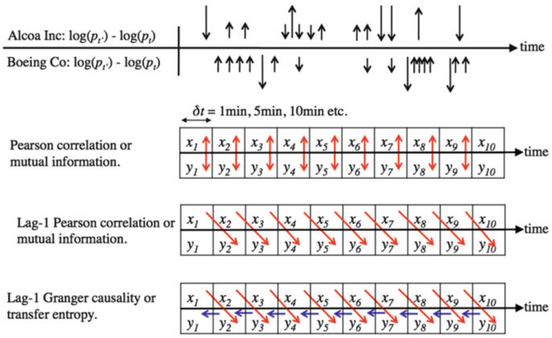
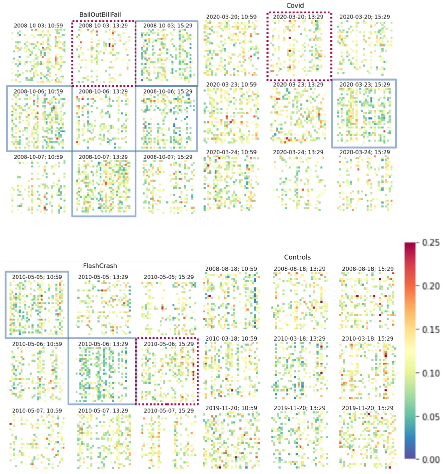
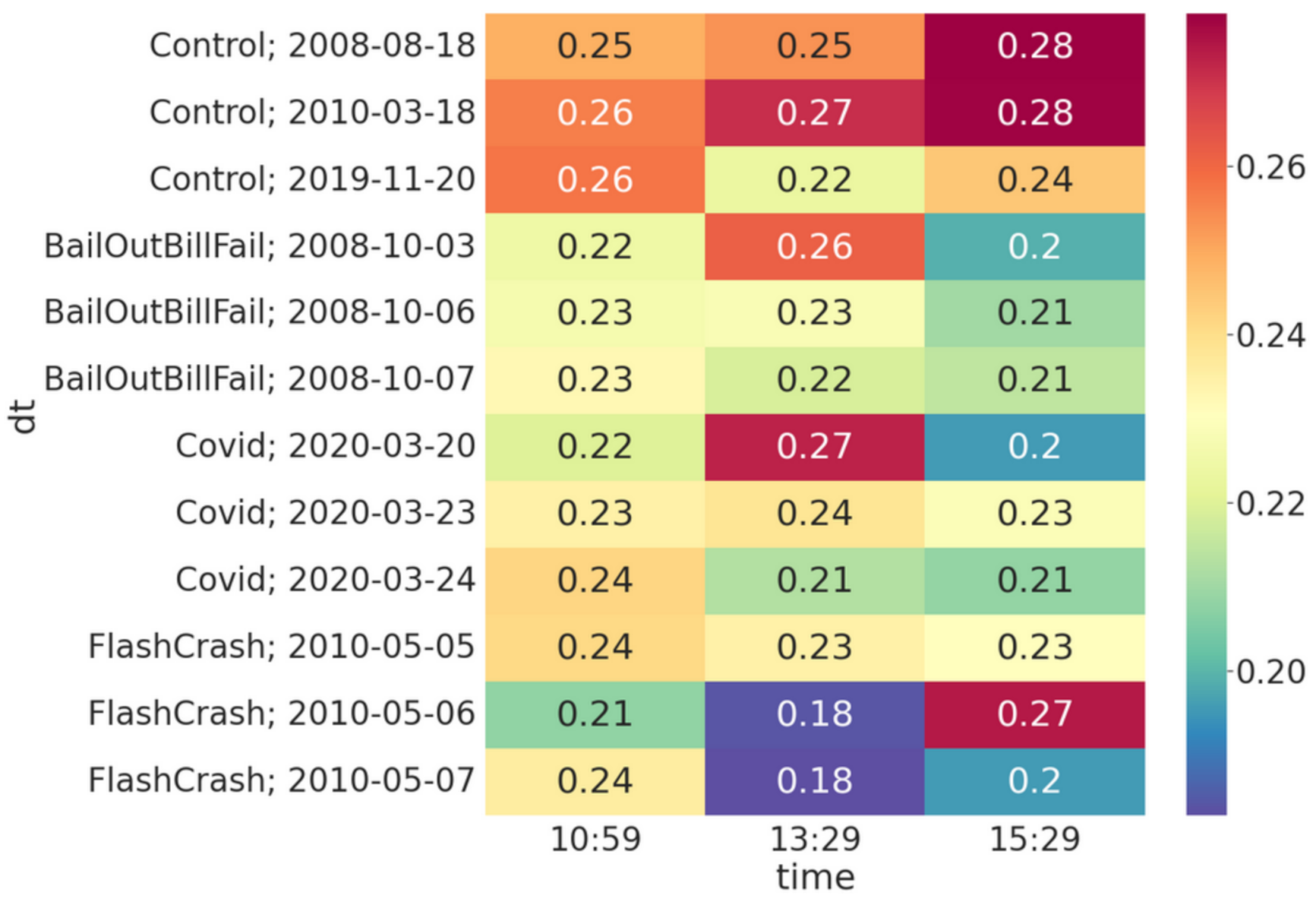
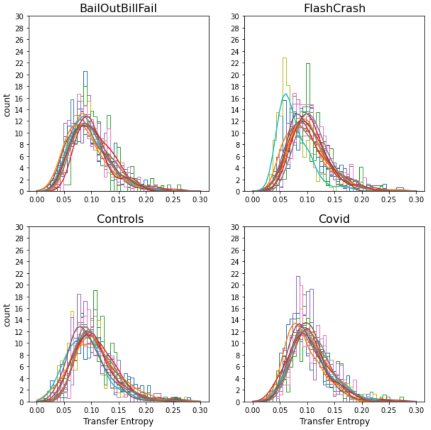
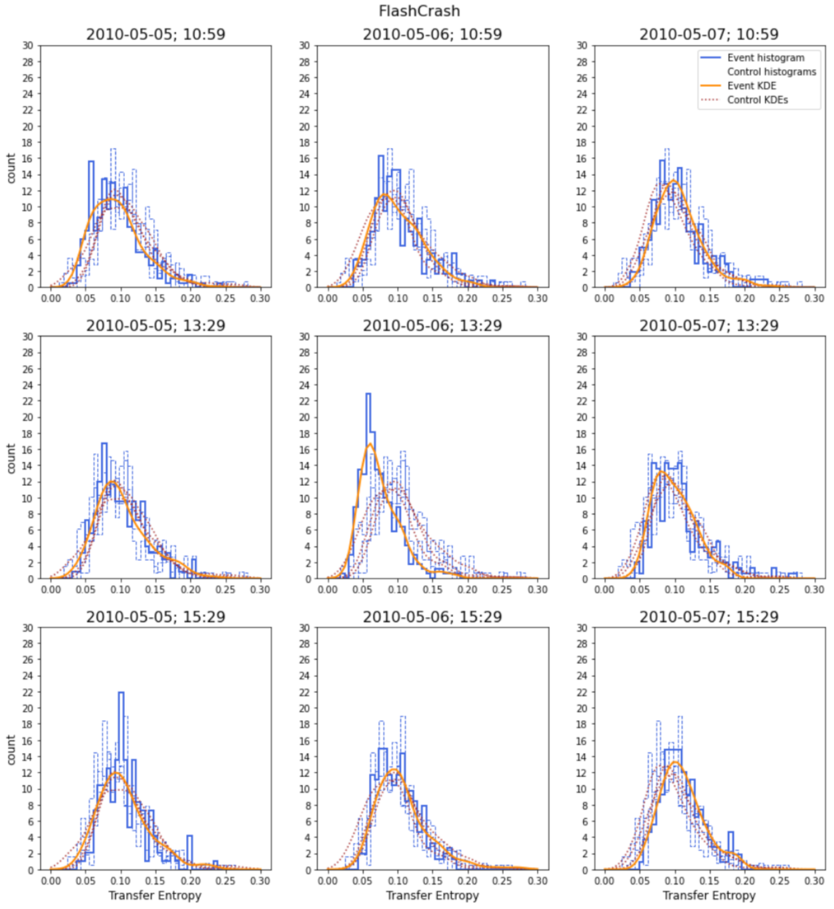
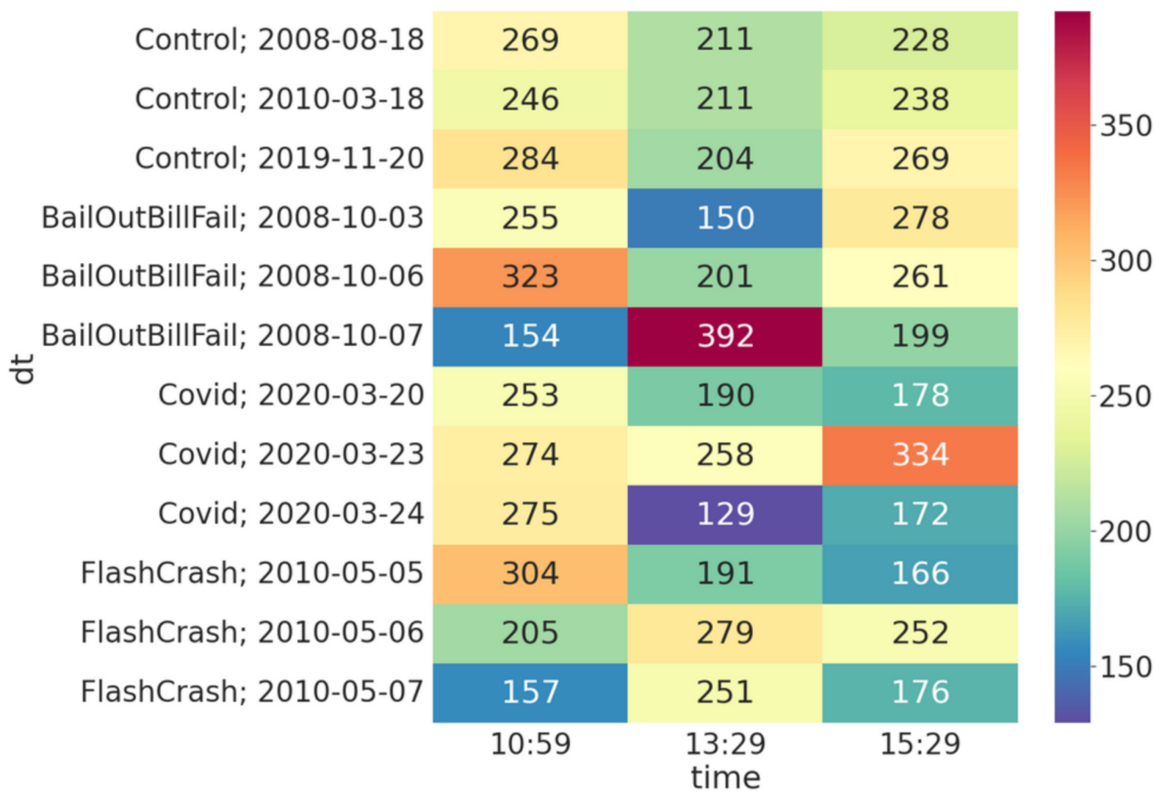
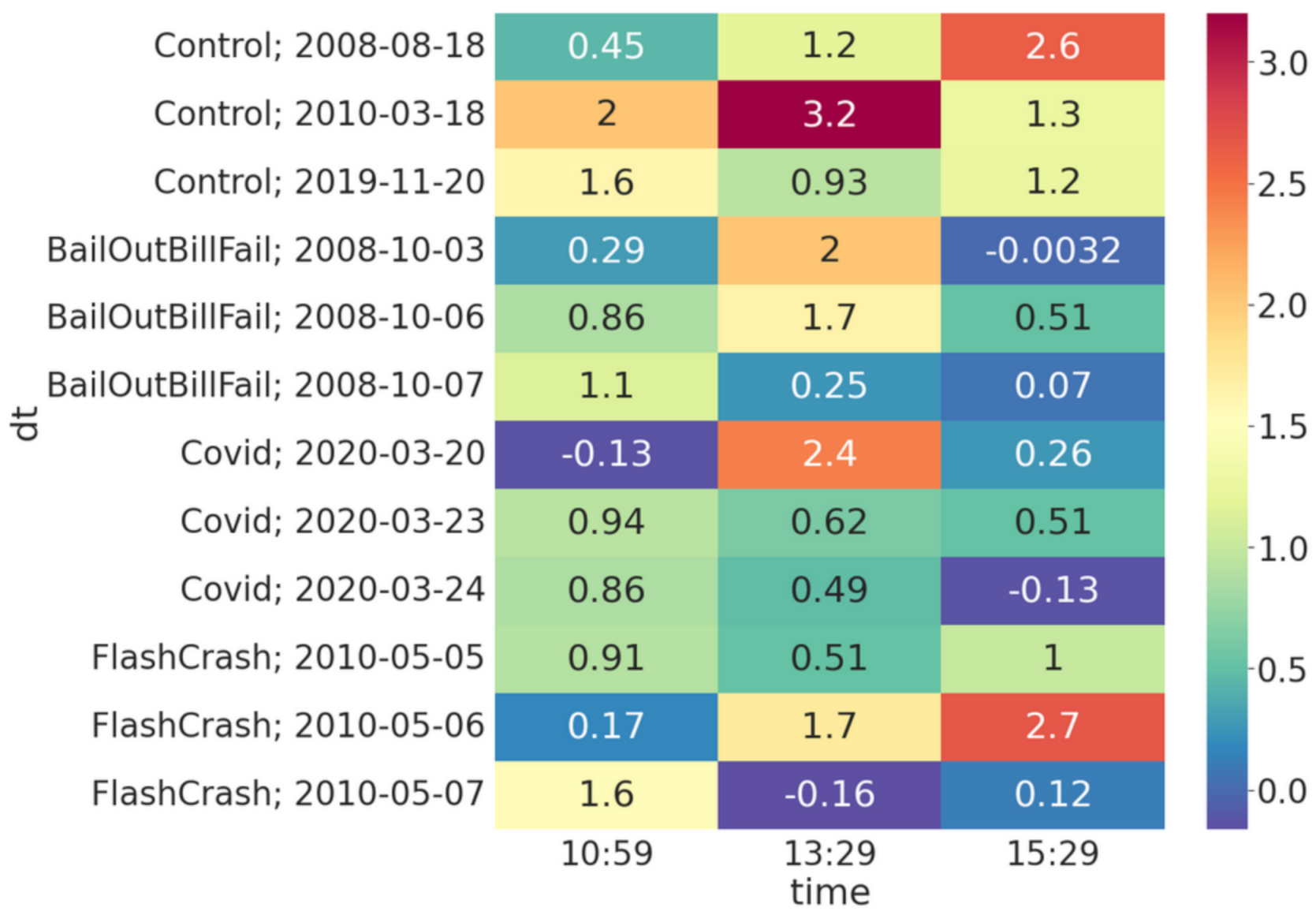
4.1. Analysis Using Transfer Entropy for the DJIA Market Shocks

The DJIA is a price-weighted index of equities for thirty of the most prominent industrial firms in the United States and as such is seen as a very broad measure of the manufacturing health of the US economy. Here, we look at this index of companies at periods covering three market events: the Federal bailout decision of 2008, the flash crash of 2010 and the COVID-19 crisis of 2020 together with three control dates where there are no recent events of any significance. For each of these market events, the analysis focuses on the day before the event, the day of the event, and the day after the event with three thirty-minute periods (backwards from 11:00, 13:30, and 15:30).
Across each of these periods, trade data for each stock were aggregated into one minute averages: d t i so that within a 1 min interval [ t , t + 1 ] we simply calculate the average price within that interval. The result is a time averaged binning of the continuous trade data over 1 min intervals and we denote this: { d t i } = { d 1 i , d 2 i , , d T i } . Subsequently, these one minute intervals are used to calculate the TE over three 10 min periods within each thirty minute window. Figure 7 illustrates the method and compares it to other common methods, but in the notation we have here for two time series of equities { d t i } and { d t j } the TE is
T j i = H ( p ( d t i ) | p ( d t 1 i ) ) H ( p ( d t i ) | p ( d t 1 i ) , p ( d t 1 j ) )
Note that this form is extended using the KSG (Kraskov, Stögbauer, and Grassberger) algorithm for effectively estimating probability distributions. A full treatment of this approach is available in An Introduction to Transfer Entropy [71].
Finally, the statistical significance is evaluated by taking the trades within each interval and reshuffling them 100 times to establish a surrogate test of the Transfer Entropy with the temporal relationships randomised. This is used to estimate the probability that the statistical significance of the obtained Transfer Entropy by reference to the randomised samples using a 0.05 p-value test for significance.
The following heat maps show the equity pairs with statistically significant values of TE, as measured by the software package JIDT [145]. Figure 8 shows the result of measuring the pairwise TE between equities in the DJIA. In each of the four time periods (each having a 3 × 3 matrix of heat-maps, top-left, top-right, bottom-left, bottom right) there are three days stacked from top to bottom (the day before the event, the day of the event, and the day after the event) and during each of these days there are three time intervals (11:00, 13:30, 15:30). Each of the 36 heat-maps is a matrix of TE from each of the 30 equities in the DJIA (rows) to each of the equities in the DJIA (columns). Periods with an increased occurrence of TE are highlighted with a light blue frame. The colour of each pixel is an indication of the size of the TE value. Periods with high maximum entropy are highlighted in red.
Looking at the event periods in Figure 8 qualitatively, entropy transmission is comparatively lower the day prior to each market crisis for all three cases. However, within those periods of fewer instances of statistically significant TE, some individual pairs produce very high values of TE. For the COVID-19 crisis, the total count of statistically significant values of TE is highest in the late afternoon of the day of the crisis (the ‘event’) although the size of the transmissions shows the largest spikes in transmission occur in the morning and early afternoon intervals. Considering the results in Figure 8 at the three market events, there are increased incidences of equity pairs with statistically significant levels of TE, however there are lower values of ’peak’ TE leading to a ‘blue hue’ for those periods of heightened activity with more active pairs but fewer high values of TE.
Looking at the count of the number of equities with high TE values during a market event in Figure 9 shows behaviour significantly different from the control sample. In the period at the end of the day prior to each market event, the occurrence of high values of TE is reduced and remains lower overall than the control periods. However, within that prior afternoon before each of the market events, there is a peak of activity when statistically significant TE values occur more frequently. This can be observed by looking at the maximum transfer entropy value for a period across the market events in comparison to the control data, seen in Figure 9.
Looking at the distribution of TE events for equities in these periods in Figure 10, the profile is similar. Across the day, an estimate of the distribution of counts of statistically significant TE values (using a Gaussian kernel density estimator) gives a peak count of transfer entropy events at any one time of twelve with a transfer entropy level of 8 to 9 bits.
However, analysis of individual periods within and around the market events in Figure 11 provides additional characteristics which distinguish the market events from the control windows. In particular, for the flash crash of 2010 we see a peak number of equity pairs with entropy transfer as an event occurs but that peak is skewed to the left indicating a decrease in the number of equity pairs with higher TE levels.
For each market event there is at least one period where the distribution has an increase in central tendency. Kurtosis measures used to capture this property have been found to be useful in these cases.
Note that this increase may not always result in changes in the kurtosis. This is because kurtosis captures the extent to which the tails of a distribution contain values greater or lesser than those that might be expected for an equivalent normal distribution. As the number of equity pairs with statistically significant TE values does change over a market event, an increase in the central tendency for the distribution is possible without a change to the tails of the distribution and the attendant change in kurtosis, see Figure 12. However, a reduction in kurtosis was observed for the population of equities undergoing transfer entropy relative to the control data (Figure 13).

4.2. Remarks

There is evidence of features in the transfer entropy activity in measures taken in and around the market events reviewed. There are similarities that can be shown with TE measures for the GFC, the May 2010 flash crash, and more recently the COVID-19 crisis. The most fruitful insights have been on an aggregate level rather than looking at calculations for individual stocks. This is in line with earlier results for the Asian financial crisis that used the same methods [70], and more generally we might expect changes in the statistics of time-series near or at a crisis point as shown in other systems [133,143] due to their very nature being that of a non-stationary event, so although these earlier studies use univariate time-series it is an interesting observation to see these changes at the multivariate and interaction level of analysis. It has also been possible to demonstrate real difference between a control population and the data from significant market events, immediately before, during, and after those events. The challenge now is to refine the calculations, gleaning clearer results with new parameters, a move from more qualitative observations to quantitative analysis and the search for real predictive capability allowing the understanding of market events through the prism of transfer entropy and associated ideas.

5. National and International Trade in Value Added

Analysing international trade as a complex network of interactions provides useful insights into the structure (topology) and dynamics of world trade and has been used to map out recent changes in trade relations. In an article by Fagiolo et al. [146], network statistics were used to determine the importance of links within the weighted global trade network between 1981 and 2000, and it was found that the majority of links were relatively weak although countries with more intense trade relationships are more clustered together. In another study by Bhattacharya et al. [40], it was shown that over a 53-year period to the year 2000 the ‘rich club’ controlling approximately half of the world’s trade has been shrinking. In a similar vein, Maeng et al. [147] used minimum spanning trees (MSTs5) to show that international trade networks were dominated by strong links between hubs of larger economies such as the USA, Germany, and China. Further progress was made by Barzel and Barabási [148] when they developed a theoretical framework (independent of its application) that uncovered universal properties of the relationship between network topology and network dynamics. This was the first self-consistent theory of dynamical perturbations in complex systems that could systematically separate out distinct contributions from the topology and the dynamics. Andrea Aria [149] from the European Central Bank has also explored how during the Global Financial Crisis the elasticity of goods exports was vastly different to that of services exports. Within such a large and varied range of new results there is considerable scope for new developments. In what follows we extend some of these ideas to networks of ‘Trade-in-Value-Added’, a relatively uncommon measure of traded value between industries and countries, in order to extract key qualitative features. For more concrete policy implications of network analysis see for example the work being carried out at INET [150].

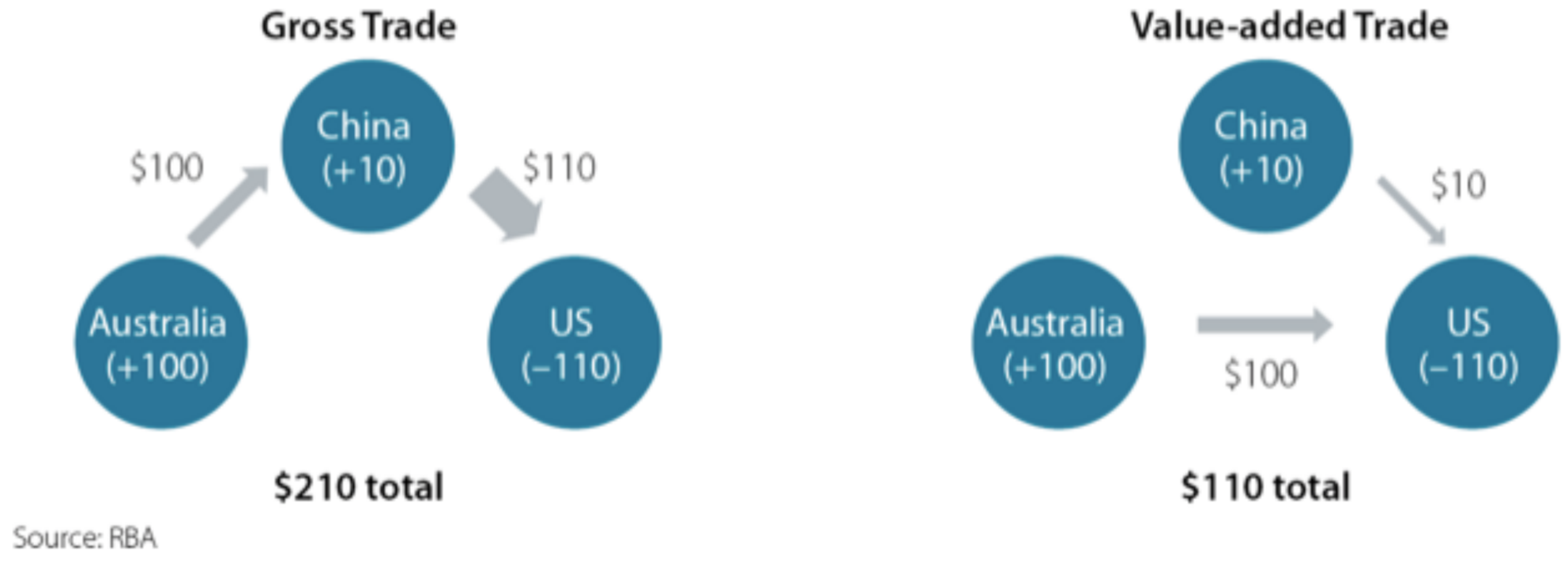
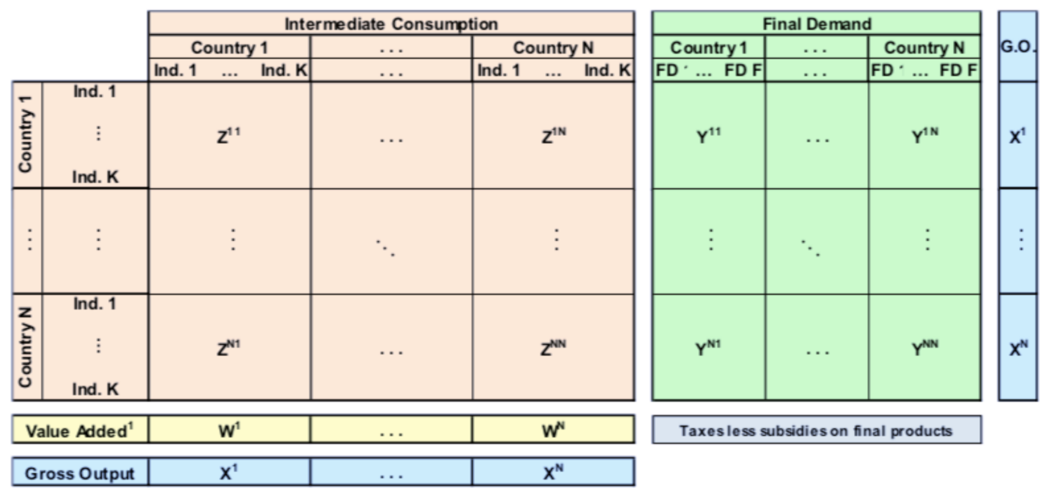
5.1. Value-Added Trade Networks

In what follows, we look at the network topology of country and industry-based trade using national and international Trade-in-Value-Added (TiVA) tables from 2005 and 2015 made available by the OECD. Nodes in a network can be either countries or industry sectors, links are between nodes are directed as they can be either originating from or terminating on a node, and in general they are not symmetric. From this we can formally represent a network as an asymmetric square matrix where the matrix entry for row i and column j, M i , j , represents a transfer of value from node i to node j, where generally M i , j M j , i .
The most common form of trade network analysis is based on Gross Trade (see the left hand diagram in Figure 14). In these networks, the cost of each good or service, regardless of whether or not it is a component in the production of another good or service (i.e., an intermediate input), is its cost of purchase which implicitly includes the cost of the intermediate goods and services used in its production. These value chains describe cumulative flows through trade networks but they offer no insights into how much value intermediate goods and services provide to the final goods and services purchased by consumers, also called final demand. Final demand plays an important part in the analysis of the national impact of an economic shock because it is used to calculate a country’s Gross Domestic Product (GDP), something that cannot be done directly from gross trade data.
To help address this, the OECD reports an alternative measure, the Trade-in-Value-Added [152], that records how much intermediate value is provided to final (i.e., consumer) demand for a good or service (see the right hand diagram in Figure 14) by both industry and country, see Figure 15. The point to note is that summations of links in gross trade networks will not reflect the true contribution of each market sector or country to GDP (compare the two totals shown in Figure 14: $210 vs. $110). Furthermore, in the analysis of economic shocks we need to distinguish between intermediate value production, which is related to employment and supply, and consumer consumption, which is related to demand, as each industry sector is made up of both intermediate products and final demand for products, and these are not symmetrical relationships but they are jointly captured in the TiVA tables. This is central to understanding the interconnected consequences of an uneven supply and demand shock like COVID-19. For example, in the article by del Rio-Chanona et al. [150], they were able to estimate
  • supply-side reductions due to the closure of non-essential industries (which can be captured in part by the intermediate value added in TiVA tables), and
  • demand-side changes caused by individuals immediate response to the pandemic, such as reduced demand for goods or services that are likely to place people at risk of infection (which is captured by final demand in TiVA tables).
From the matrix shown in Figure 15, we can see that the OECD tables can be split into two parts: the internal economic structure of a country, represented by the trade between industry sectors within each country, and the global trade in value, which we will capture by aggregating total values traded between countries. In so doing, we can begin to understand how both local and global value chains are impacted by economic crises.

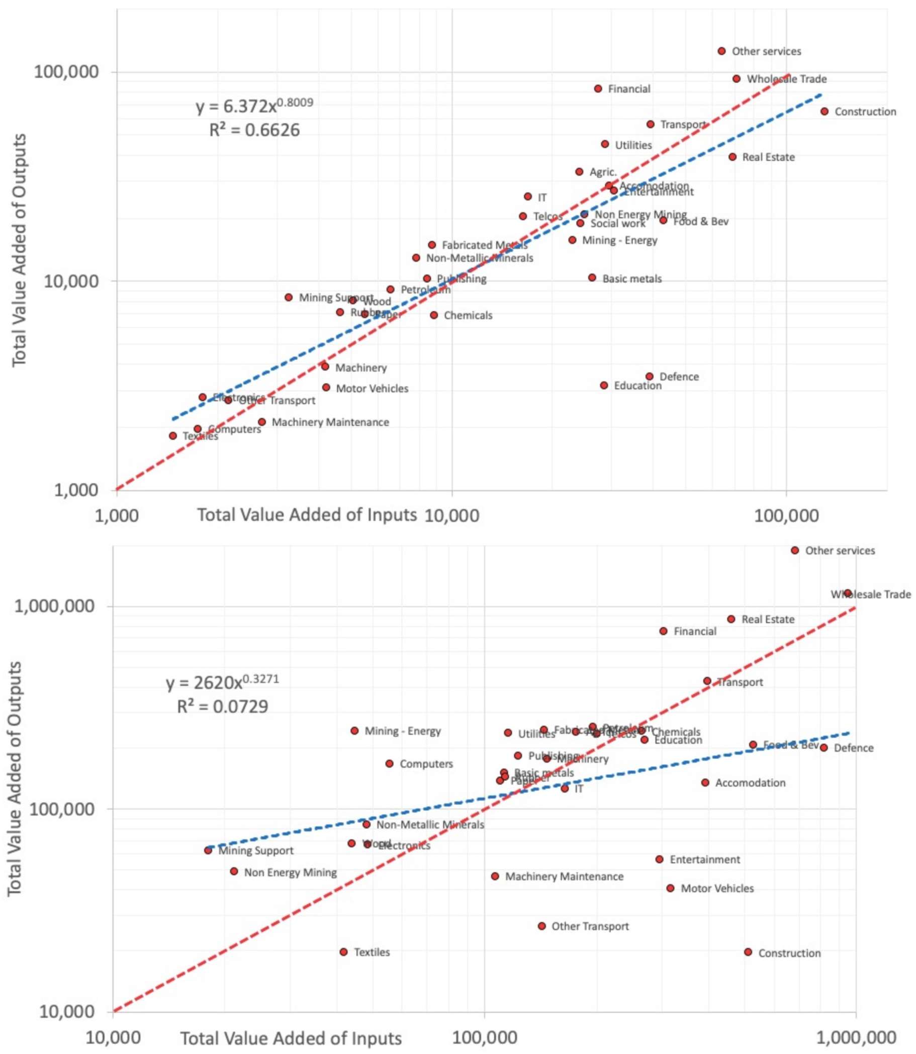
5.2. Features of Australia’s Internal Trade Patterns

Looking at the local value chains for Australia, we study the total contribution each market sector makes to every other market sector by summing the entire row of each industry (in the TiVA data tables) and in measuring the contribution made to an industry we sum each industry’s entire column (also see Figure 16 below). This captures the total consumption of value (final demand) of each market sector and the total production of value (value added) of each market sector, and so we can plot the relationship between these two aspects of a market sector by value on a single diagram, as shown in Figure 17.
In Figure 17, we analyse Australia and compare it with that of the U.S. using data that were obtained from the OECD’s TiVA database of input–output tables.7 In these plots, the x-coordinate is the total value of final demand of value in each market sector: it is the sum of all value contributed from other market sectors that contribute to the final demand of each individual market sector indicated on the plot. The y-coordinate is a proxy for the supply side of value each market sector provides to the final demand of the rest of the economy, calculated by summing the value added by each sector to all other sectors.
In Australia, we observe that the supply and demand is reasonably well balanced: sectors with low values of total inputs are closely related to sectors with a low value of total outputs to the rest of the economy. On the other hand, high-valued input sectors also have high-valued outputs ( R 2 = 0.6626 ). In these terms, supply and demand of value in the national value chain of production are reasonably well balanced and a shock to each sector is likely to have an equivalent impact on both the supply side and the demand side of value. The two notable exceptions are education and defence that have a relatively high supply side of value but a relatively low value of demand side of value.
The U.S. tells a very different story to Australia in terms of its internal economic structure. There is very little relationship between the demand side of value and the supply side of value ( R 2 = 0.0729 ), and a number of industry sectors such as entertainment, construction (and other heavy industries), and transport have greater demand of value than supply of value. On the other hand, real estate, wholesale services, and other service are more similar between the two economies (once differences in the total size is accounted for). Of course this is only the internal structure of the economies and the relationship between industry sectors and their international trading partners, as expressed in the value of overseas final demand and overseas contributions to internal final demand still need to be accounted for in order to have a more complete economic picture.

5.3. Predicting the Impacts of Exogenous Shocks

Now that we have a framework for understanding the structure of trade, we want to analyse how this structure might be impacted by exogenous shocks such as COVID-19. The dataset is reduced to Australian-only input and output industries using a Domestic Industry Sensitivity Matrix, see Figure 16. The matrix is a topological representation of the trade input-output function of each industry which allows quantitative, structural analysis of important relationships between industries as well as the impacts of first and second-order flow-on effects from perturbations in inputs or demand functions. For example, we can see that Transport, Utilities, and Wholesale Trade contribute value to final demand for almost every other sector in Australia, and Construction, Defence, and Education receive value to their final demand from a large part of the Australian economy.
To demonstrate how the sensitivity matrix can be interpreted, we analyse the first-order demand and supply effects of a 10% reduction in construction output. Table 1 and Table 2 summarise the top 3 most-impacted industries from a notional value basis and a relative basis (as a concentration of impact that industry has relative to trade with all other industries).
As the fall in construction affects the demand for input industries, we can analyse the subsequent output effects of a fall in construction on industries that rely on construction as an input.
These are just the first-order supply and demand effects of a temporary perturbation in the demand and supply for an industry based on the internal trade of the Australian economy. Longer-term impacts will propagate into second-order effects which can be analysed using the sensitivity matrix.

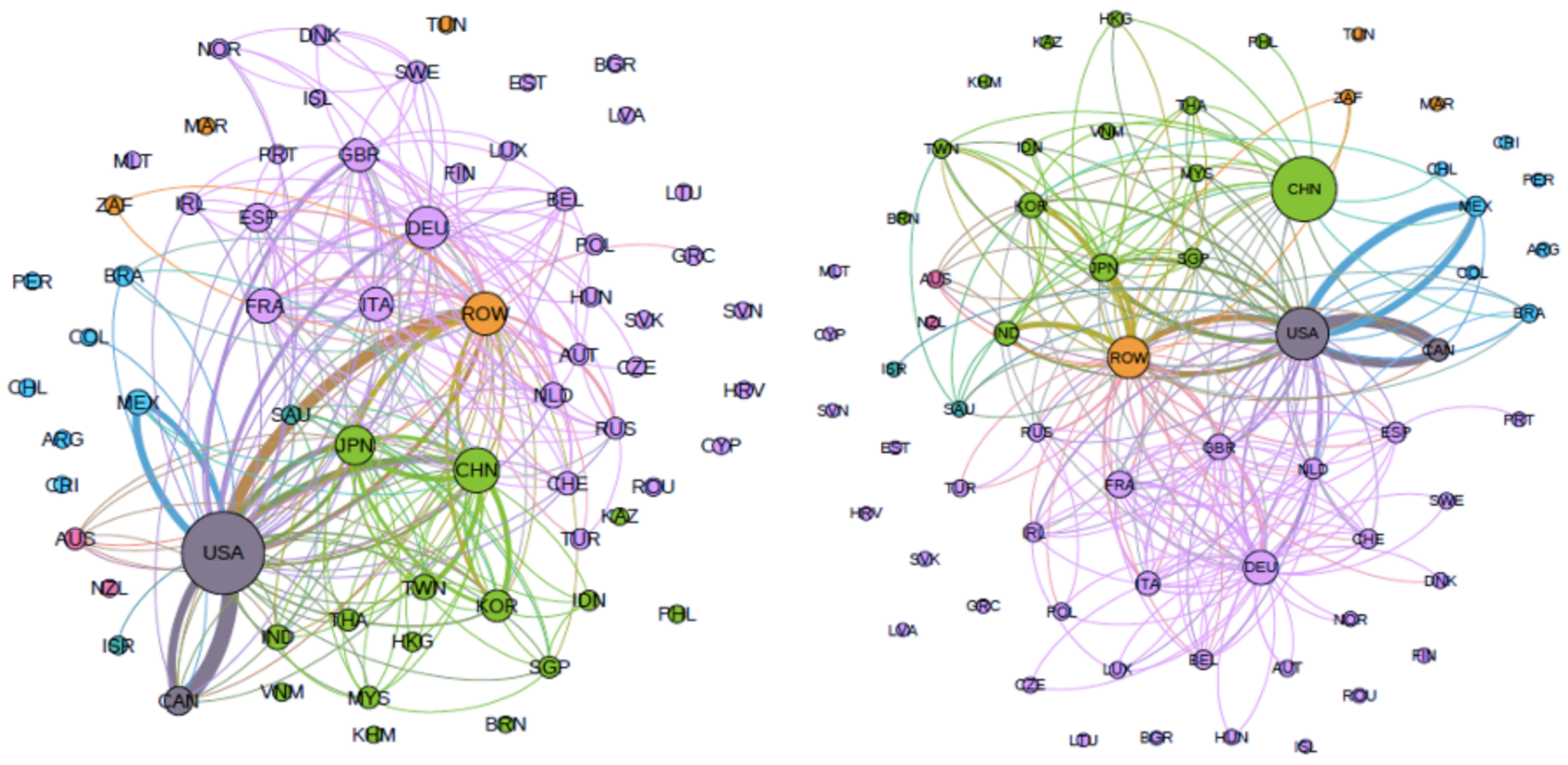
5.4. Features of Global Trade Patterns

The global patterns of trade between industry sectors and countries is a complex, multiply layered network of interactions and so to simplify our analysis we only study the total values of trade between countries. In Figure 18, we show the total trade in value added between countries for 2005 (left) and 2015 (right) from which we can extract some qualitative features, noting that the node representing the rest of the world (ROW) has been held approximately constant so that we can compare relative changes in the other countries.8 We can clearly see that the USA’s export influence has declined in these 11 years while China has increased, matching the results of other work, for example, Deguchi et al. [153] have reported that between 1992 to 2012 the USA decreased in global trade authority while China has increased and recently surpassed the USA in this respect. We can also see that the ROW has become a more central element in the network, having a weaker relationship with the USA but a stronger role to play in trade with other region of the world. Other features are also evident: Japan and a number of European countries have decreased in value added trade while Korea has increased. One aspect of the structural change in trade dynamics has been the emergence of intraregional trade and regional supply networks, see, for example, Kelly and La Cava [151] and Zhu et al. [154]. This can be seen in Figure 18 where the global regions are colour coded and segmentation of the networks by regions is apparent.

5.5. Remarks

The motivation for this analysis has been to explore how a complex network-based system can represent the characteristics of an interconnected global trade network at the global, country, and industry levels. By probing network structures at these levels through matrix sensitivity analysis and changing patterns in global trade, we have a method to explore the potential demand and supply shocks that propagate through national and global networks. Further work can extend these methods to incorporate occupations, geographies, and work activities involved within each industry which would assist government policymakers in crisis response, a process that has already begun with the work being carried out at places such as INET.9 Another consideration not explored in this research is that of the elasticity of industry supply and demand functions which would impact the magnitude of exogenous shocks, see, for example, the work of Escaith et al. [155] on the impact of the global financial crisis on trade networks.

6. Project Economics and the Knock-On Macro-Effects of Their Delay, Cancellation, or Failure

Central to the economic development of a country is the delivery of innovative products as well as the infrastructure necessary for economic expansion, such as roads and power stations. From the view of an organisation though, projects are an important organisational construct used to plan and control the delivery of a vast array of products and services [124,156,157,158]. By definition, a project is a temporary activity undertaken to create a unique product, service or result [159]. As temporary forms of organising, they have the potential to generate innovative capacity and strategic flexibility [160]. Quantifying the number and scale of projects under management within a country or across the world is difficult, but based on a study of three Western European countries it has been shown that the degree of projectification of an economy relative to the gross domestic product is in the order of 30% [161]. This provides us with the motivation to better understand the effects of crises on project development and deployment in the context of the economic growth of an economy.
Organisations vary in the degree to which they engage in and describe their work as project focused. Yet, projects are increasingly being employed as a tool of strategic innovation in all industries: for the delivery or development of their products or services for their customers, the transformation of their own structure or culture, or the design and implementation of their strategies [124]. Broadly speaking, organisations can be separated into at least two categories: project-based organisations and project-oriented organisations. Furthermore, some firms offer complex and individualised solutions to their customers that are contracted before project development starts [124]. Turner and Keegan [162] have argued that these firms are project-based because of the customised demand of their clients. On the other hand, some organisations choose to become project-oriented as a matter of strategic choice [124].
Although there is no formal convention differentiating the types of projects undertaken by these organisational typologies, there is arguably an intuitive distinction to be made. If an organisation is project-oriented, the undertaken projects are often numerous and small in scale (e.g., local, short-term, and lower cost). Project-based organisations, in comparison, are often found to be involved in the delivery of large-scale investment projects with a significant degree of complexity. If a project is sufficiently costly (>US$ 1 billion), spans over several years, and is expected to have a significant societal or economic impact, it is termed a megaproject.
Project-oriented organisations may have tens to hundreds (or even thousands) of projects underway for many different clients, internal and external, at any given time. This large number of concurrent projects presents several portfolio management challenges, including the identification of, and intervention on projects that go off track during delivery [60]. In these portfolios, each project, and its expected outcomes, is important enough in its own right to demand the time and resources needed to sustain it, but it is unlikely that the delay, cancellation or failure of one or even a few projects will threaten the overall success or survival of that firm.
The same is not true for project-based organisations, which may have just one or two very large, long, or complex megaprojects under management at any given time. Many other partner, supplier, and subcontractor organisations may be engaged in these megaprojects. Therefore, the delay, cancellation, or failure of any one of these projects may have a significant impact on the survival of the delivering organisations, and have a much broader impact on the economies, environment, or even societies for whom they were being delivered [163]. Flyvbjerg ([125], p. 6) defines megaprojects as being “large-scale, complex ventures that typically cost US$1 billion or more, take many years to develop and build, involve multiple public and private stakeholders, are transformational, and impact millions of people”. Megaprojects are used as the preferred delivery model for infrastructure, water and energy, mining, enterprise systems, mergers and acquisitions, space exploration, the development of new aircraft, airports, drug development, national broadband, and Olympic Games [125,126,127].

6.1. Mega-Projects and the Economy

Megaprojects facilitate the implementation of technological and organisational innovations at a scale that is usually inaccessible to most organisations. Edward Merrow in Flyvbjerg et al. [164] (p. 4) wrote:
… such large sums of money ride on the success of megaprojects that company balance sheets and even government balance-of-payments accounts can be affected for years by the outcomes. The success of these projects is so important to their sponsors that firms and even governments can collapse when they fail.
This extreme scale is reflective of the functional complexity of megaprojects which are themselves often initiated to facilitate the productive efficiency and delivery of many other goods and services. It could be argued that megaprojects emerged as a managerial concept to solve the problem of delivering such complex projects where previously existing project management practices were found to be inadequate. As their inception, much has gone into developing and disseminating megaproject theory in a cycle that has neo-Shumpeterian attributes [165,166].
Megaprojects stand out for another important reason: they are plagued with overly optimistic estimates of time, costs, and expected benefits [126,164]. While optimism bias is not unique to megaprojects, given the scale and import of these projects these underestimations have greater impact. This is well illustrated by the cities competing to hold the Olympic Games, which have consistently underestimated and yet these errors have been repeated every four years [126]. In their working paper, Flyvbjerg and Stewart [127] studied the cost overruns of the Olympic Games from 1960 to 2012. They found that the Games projects overran with 100 percent consistency. They explained that other types of megaprojects experience cost overruns from time to time, but none were found to be this consistent. Additionally, Flyvbjerg and Stewart [127] reported that the Games cost overruns of well over 100 percent, was significantly larger than for other types of megaprojects including infrastructure, construction, information, and communications technology.
Further, the environmental and social effects of megaprojects are commonly found to have been miscalculated or not taken into account at all, and surface during construction and operation, potentially destabilising habitats, communities and the projects themselves [164]. Adding to systematic underestimation, decision making around megaprojects is further impacted by deception and delusion, in the form of strategic misrepresentation by project promoters [164], and exacerbated by misplaced political incentives [126] or political ambitions [167]. Referring to infrastructure megaprojects, one of the arguments commonly made by project promoters to commit public funds is that these projects will generate economic growth in a particular region, country or local area, but these expected regional benefits repeatedly turn out to be unquantifiable, insignificant or even negative [164].
When faced with an economic downturn, project-based and project-oriented organisations may be impacted in quite different ways depending on the nature of their projects and their respective products, services, and customers. In their favour, Aritua et al. [168] argue that projects are complex adaptive systems, and as such project managers and their project teams are always reacting to the changing environment around them. On the other hand, some changes to a project’s environment are so large and disruptive that this more organic response may not be able to respond adequately to protect the project and its deliverables.

6.2. COVID-19 at the Project Level

Due to their extreme scale and impact, megaprojects may play a significant role in shaping the (socio-) economic processes of an economy. However, the reverse may also be argued, i.e., where there is an economic disruption like that caused by the COVID-19 pandemic, this can precipitate the cancellation or pausing of megaprojects as their funding bodies reassign previously budgeted capital to other more pressing needs with the resultant loss or delay of innovation and value. Early investigations into the impact of COVID-19 on construction projects in the USA [169,170], UK [171], and New Zealand [172] show that within months of the declaration of the global pandemic, construction companies were seeing large numbers of projects cancelled or put on hold. A report from July 2020 shows that in the United States roads and transportation projects alone, projects to the value of US$9.6 billion had already been delayed or cancelled. As of July 2021, the US state of California was reporting 35 cancelled construction projects (US$ 131 million), 580 delayed projects (US$ 6.03 billion), and a further 224 (US$ 6.7 billion) that have been put on hold due to COVID-19 [173]. Between September 2019 and 2020, construction sector employment in the US decreased by 275,000 year on year [174], recovering from peak employment losses between March and April 2020 of approximately one million workers [175].
This disruption to the project delivery pipeline can be expected to cause several levels of disruption. At the local, regional, and national levels, there is the short-term disruption to local spending on raw materials, goods and services to support projects, and the employment of local labour. In the longer term, the discontinuance of these projects may have far reaching impact due to the delay or non-delivery of the expected benefits of the project. This impact could be felt in slowed or limited urban or rural development, agricultural growth or regional tourism to name a few. In this way, the shorter term savings accrued through the cancellation or delay of a large infrastructure project may be significantly outweighed by the longer term losses mentioned here. Further, there is a significant disruption to the delivering organisations, where firms that design, plan, and deliver these projects are faced with a severe disruption or cessation of expected cash flow, discontinued access to the work site and to the labour needed to complete the work. At the same time, if the project is expected to be continued in the future, these firms are faced with several dilemmas on how to continue to make their project financing payments and leases on critical equipment, and how to retain access to skilled labour when it is not clear when they will be needed again.
The broad and almost simultaneous geographic impact of the pandemic has created a unique situation where specialised firms that might ordinarily have moved resources from one project to another when one was cancelled or delayed may now find themselves with very few continuing projects to work with. Faced with this project pipeline contraction, delivering organisations may decide to take protective actions by laying off employees and other cost reduction tactics. These tactics may serve to preserve the organisation in the short term, however, when project work eventually recovers they may find it difficult to recover lost productivity and talent that these temporary reductions caused. The reduction of the work force itself also has an impact on household incomes for the affected workers, thereby affecting the national economy’s final demand just as in the case of many other industries, see Section 5 for a more detailed analysis of the impact that job losses can have on an economy.
As some countries begin to emerge from the grip of the pandemic, there are moves to spur economic recovery by initiating large infrastructure projects.10 Just as the almost simultaneous contraction of project demand caused delivering organisations to make changes in staffing and spending en masse, starting (or restarting) significant numbers of very large projects over a short period will likely stress delivering organisations as they seek to rapidly revive their projects and recover their work forces while simultaneously competing for newly announced projects in these infrastructure spending measures. Further, this restart may cause several other issues, such as the competition for skilled labour resources who would ordinarily move from project to project as they asynchronously started and ended may now be sought by many delivering organisations who are restarting projects at a similar time.

6.3. Remarks

In this section, we have described how the impact of one or more projects being delayed, cancelled, or failing in organisations that deliver multiple simultaneous projects to many different customers were comparatively small as they only make up a small part of a much larger portfolio. In this case, when one project fails, losses are somewhat easier to accept, and now-surplus human resources may be assigned to other projects in the portfolio. However, if a large portion of those smaller projects were being delivered to one of the more heavily impacted sectors, a large portion of the portfolio might need to be suspended, and may not be reinvigorated when the crisis has passed. In this case, the an organisation may not be able to afford to support the workforce during this period of reduced activity, which may result in layoffs and other cost reduction tactics.
The scene is different for megaprojects whose delivering organisations might have just one or a few megaprojects underway. These megaprojects are already risky prospects, and due to their long planning horizons and delivery timelines, they are particularly exposed to extreme events with large negative outcomes i.e., “black swan” events [125] such as COVID-19 or the 2008 Global Financial Crisis. Despite their devastating effect when they occur, megaproject (and indeed smaller project) managers generally ignore the possibility of black swan events in their planning [125]. We discussed above how big a megaproject might be, and how reliant the delivering organisations and even governments can be on a project’s success. Given the economic impact on the region as well as the local and global workforce, it may not be possible to put a megaproject on hold. However, even if the project has the funds to proceed, it may be faced with other issues due to social distancing requirements that affect work site staffing, or the lack of access to expert resources who may not be able to travel to the site of a project, or shortages of raw materials as global supply chains respond to rapidly increasing demand, stressing already compromised global value chains (which we discuss further in Section 5). Even if a megaproject could be stopped altogether (which is unlikely to be a contractual option [125]), in times of economic downturn the injection of capital into the economy through local employment and other locally procured services might provide some stability to augment national level stimulus packages.

7. Conclusions

While all economic crises are idiosyncratic in the details of their cause and effect, the interactions between heterogeneous agents are integral to understanding the life cycle of a crisis-instigated market failure. This point is central in both the general development of ‘complex systems theory’, see, for example, Barzel and Barabási’s work [148] on the interplay between topology and dynamics for perturbations to networks, as well as specifically in complexity economics, for example, Arthur’s recent overview [21]. There are two ancillary arguments captured by the present article in support of this primary claim. First, the particular way in which agent heterogeneity is expressed is crucial in the precipitation of market conditions. This is because the topological structure of economic relationships is significantly influenced by the type and degree of difference displayed by agents. Second, in the absence of complete information, market interactions with an inter-temporal component are significant to the precipitation of a crisis-like event. Unanticipated events that prompt a sudden increase in agent uncertainty are essentially ‘information shocks’ that have the potential to prompt a cascade of maladaptive agent responses that are ‘baked in’ through long term contracts and other inter-temporal mechanisms. Agent heterogeneity and inter-temporal interaction, in other words, inform how destabilising forces unfold in a market environment.
The article applies these interactionist principles to analyse markets at varying levels of aggregation. At the most fine-grained level, we have the pure simulations of Section 2, where, due to the model’s purely theoretical nature, we have complete control over the states and interactions of the agents, essentially an entire economic reality within which we can explore every aspect of every agent. In Section 3, we are one step removed from the purely theoretical by introducing socio-economic data from a the Sydney housing market while maintaining complete control over the individual agents we populate the model with and the methods by which they interact with one another while still requiring that their behaviour reflects observable dynamics. In the section on financial markets, Section 4, we move even further away from the specifics of the agents, and we infer that some form of interactions are taking place between individual agents (equity traders) in the market and that we can measure these interaction and so infer a network from observed price behaviours. At the most coarse-grained level of Section 5, we look at national and international trade networks where all notion of individual agents are essentially lost and all we have available to us are the aggregate values of final demand and value added between market sectors and countries. In our final section, Section 6, we look at the role of projects as institutional structures and as mechanisms of economic development, where the relationship between multi-billion dollar projects and economic progress is writ large and is often specifically political in the way they embody and make visible the economic direction and ambitions of a nation.
Each of these economic layers has, to one degree or another, an underlying representation of heterogeneous economic agents. It is also well established in the economic literature that agent heterogeneity and inter-temporal exchange under uncertainty can propagate economic shocks through market networks [176,177]. The intellectual fine-print here is that these issues have historically been studied as autonomous problems, more often than not relegated to the realm of pure theory (although the two references provided here are notable exceptions). In cases where agent heterogeneity is considered within an inter-temporal exchange framework, analysis is typically limited by the methodological constraints of analytical tractability that is often expected in orthodox economics. In the economic discourse around crises, model tractability is a uniquely pernicious concern, as the success of an economic model has historically been evaluated in terms of the existence of a unique stable fixed-point equilibrium [49], or now more commonly, a stable steady state. Although it is uncertain how the institution of mainstream economics will shift in a post-COVID world, much of the methodological conventions considered standard economic practice developed with the belief that economies can be persistently efficient if the appropriate market mechanisms are in place. There is reason for optimism though. In a 2021 survey of articles on the economics of COVID-19 by Padhan and Prabheesh [178], they report a large number of studies using conventional economic methods (difference in difference, GARCH, descriptive statistics, etc.), but they also found methods similar to those described in this article have also been used, such as Granger causality, correlation-based minimum spanning trees, and trade network analysis (using artificial neural networks). This indicates that along with the crisis is coming a greater diversity of approaches to modelling and empirical analysis, which we would argue bodes well for both traditional economics and complexity economics.
In our opinion, CE represents an epistemological maturation of economics, in that it connects the social sciences to a broader corpus of scientific knowledge. This imposes a sufficiently theoretically agnostic and externally accepted standard of analysis to which the practice of economics can be measured against and verified by. As many of the methodological conventions within CE have been developed, applied, and verified in multiple non-economic disciplines, CE is also methodologically consistent. The principles associated with CE methods are mutually supportive and more importantly, do not typically contradict. As a result, the complexity framework is more data-orientated, tends to be testable, and is also flexible relative to, for example, the axiomatic structure of general equilibrium models. We hope and even expect that out of the current crisis will come a broader acceptance of new economic methods and theories that will have the opportunity to be developed and refined before the next crisis so that, when it does inevitably arrive, we will be better prepared with sound policy advice.

Economic Research on a Global Scale

Another very important task that has been carried out during this pandemic is the curation of data and research into central repositories for the benefit of other researchers. One such repository of economic data relevant to COVID-19 is the Data Resources for Socio-economic Research on COVID-19 page maintained by the European University Institute [179]. On this website can be found sections such as Macro-financial systemic impacts and links to key databases such as the Eurostat database that gathers statistics on the economy related to COVID-19 [180].
In addition to curating data groups, they have been curating research papers related to the economics of the pandemic, such as the work of CEPR (Centre for Economic Policy Research) that has gathered, vetted, and published COVID-19 economic papers since March 2020 [181]. The variety of subject matter and methodologies covered by the different research programs across the globe is evident in this extensive library of material and we briefly discuss four of them here. At the level of an individual’s interaction with the disease and policy, vaccine policy features prominently. For example, the paper by Turner et al. [182] studies the race between the emergence of new COVID variants and the roll-out of vaccines, estimating that
… fully vaccinating 50% of the population would have a larger effect than simultaneously applying all forms of containment policies in their most extreme form (closure of workplaces, public transport and schools, restrictions on travel and gatherings and stay-at-home requirements). For a typical OECD country, relaxing existing containment policies would be expected to raise GDP by about 4–5%.
Stimulus packages also feature significantly in the database of articles, for example, Falcettoni and Nygaard reviewed the literature [183] on stimulus payments in the US in response, concluding in part that
… the poor and the young, especially those with children, should have received a larger [economic stimulus] check, which is an allocation that would have allowed for the same stimulus effect at half the cost of the actual allocation [as delivered by the US government].
Another key area of research highlighted in these articles is the impact of the pandemic on stock markets. On this topic, an article by Capelle-Blancard and Desroziers [184] showed a number of interesting results regarding the extended evolution of market response to the pandemic and the heterogeneity of its impact across 43 economies (dates in 2020):
  • Stock markets initially ignored the pandemic (until 21 February), before reacted [sic] strongly to the growing number of infected people (23 February to 20 March), while volatility surged and concerns about the pandemic arose; following the intervention of central banks (23 March to 30 April), however, shareholders no longer seemed troubled by news of the health crisis, and prices rebound all around the world.
  • Country-specific characteristics appear to have had no influence on stock market response.
  • Investors were sensitive to the number of COVID-19 cases in neighbouring but mostly wealthy countries.
  • Credit facilities and government guarantees, lower policy interest rates, and lockdown measures mitigated the decline in domestic stock prices
A final common theme reported in the CEPR database is the work on the economic impact of lockdowns. In a paper by Caselli et al. [185], they reported that their is a dual mechanism in play over the first seven months of the pandemic, one due to state enforced lockdowns and the other through voluntary social isolation in which people acted of their own accord to help mitigate the effects of social interaction on the spread of the disease. Further, they were able to estimate the differences between policies:
We also show that lockdowns can substantially reduce COVID-19 infections, especially if they are introduced early in a country’s epidemic. Despite involving short-term economic costs, lockdowns may thus pave the way to a faster recovery by containing the spread of the virus and reducing voluntary social distancing. [They were also able to show that the effect] … entail[s] decreasing marginal economic costs but increasing marginal benefits in reducing infections.
Results such as these have a clear interaction between government economic policy and public health, a rich interaction that helps clarify many of the difficult public policy debates that often pit economic and health factors against one another.
As a final point, we consider the potential for long term economic impacts of extended health issues that are the result of so-called ‘long COVID’ [186]. There has been a growing awareness of the long-term negative health outcomes caused by a cluster of medical conditions such as shortness of breath, muscle aches and pains, and overall tiredness. These chronic physical manifestations of contracting COVID-19 may result in long-term reduction in individual financial stability due to the potential for job loss, long-term disability, and the increased burden of medical costs. This reduction in economic health alongside the reduction in overall quality of life may be one of the greatest long-term economic and social pitfalls of chronic COVID-19-related illnesses. It is also important to note another, less well-studied, impact of long COVID, the long-lasting cognitive deficits that come from even relatively mild symptoms of the disease. In a recent study by Hampshire et al. [187], in which 81,337 UK residents carried out a cognitive test and then reported on their COVID-19 status (asymptomatic and not biologically tested, suspected infected but not biologically tested, infected and confirmed with biological testing, admitted to hospital but not ventilated, admitted to hospital and ventilated), they found that nearly 25% of people who had contracted the disease suffered from at least some form of long COVID. While this is concerning enough, they further showed that of those patients that were not admitted to hospital but were biologically confirmed to have had the disease the cognitive impact was the equivalent to that of having had a stroke and being admitted to hospital and ventilated was equivalent to a 7 IQ point impairment. While these are worrying results, it is slightly less worrying if the disease is confined predominantly to older members of the population where training, experience, and financial and professional stability may provide some reduction in the overall impact on quality of life and long-term financial outcomes, but it is less reassuring for younger people who are more at risk from recent variants of COVID-19. This risk led US President Joe Biden on June 18 (2021) to urge young people to be vaccinated to protect them against the new delta variant [188]. The lifetime economic and total quality of life impact of COVID-19 is not yet well understood, but for younger people the lifetime loss of earning power and productive ability is much greater than older patients, a fact that may be the cause of the most long lasting effects of this pandemic.
What we have sought to show with these case studies are some of the main effects and spillovers of a crisis and that this research is also part of a larger, diverse, and significant push to understand the global impacts of the COVID-19 pandemic. One of the points we have particularly emphasised is that, in response to crises such as this, the mainstream view of ‘economic agents’ needs to be broadened to fully account for the individual’s biological, psychological, and sociological characteristics that underpin their fundamentally non-stationary, dynamic nature, and that, as such, economics when it is most needed during a crisis needs to account for society’s distinctly non-equilibrium nature. This is almost by definition an ‘out of sample’ task with significant spillover effects: there is no historical context to readily draw upon and one country’s changing health policy can be another country’s economic crisis. Once we take these issues seriously and begin to put more significant resources to the task of understanding the complexity of our socio-economic systems there is a great deal of room for us to improve our ability to respond to future economic developments, both in and out of a crisis.

Author Contributions

Conceptualization, M.S.H.; Data curation, A.E., K.G., L.P., and S.W.; Formal analysis, M.S.H., A.E., K.G., L.P., and S.W.; Funding acquisition, M.S.H.; Investigation, M.S.H., A.E., K.G., M.H., L.P., S.W., and L.C.; Methodology, M.S.H., K.G., and S.W.; Project administration, M.S.H.; Software, K.G., L.P., and S.W.; Supervision, M.S.H.; Validation, K.G., L.P., and S.W.; Visualization, M.S.H., A.E., K.G., L.P., and S.W.; Writing–original draft, M.S.H., A.E., K.G., M.H., L.P., S.W., and L.C.; Writing–review and editing, M.S.H., and L.C. All authors have read and agreed to the published version of the manuscript.

Funding

This research received funding from the Australian Research Council grant number: DP170102927.

Data Availability Statement

All publicly available data used in this work is available at the links provided in the manuscript. Proprietary data has also been sourced from SIRCA/CoreLogic for the Australian housing ABM and used with their permission.

Acknowledgments

We would like to thank Kimberley Yoo for helping in reviewing the economic content of the article. Data on housing transactions are supplied by Securities Industry Research Centre of Asia-Pacific (SIRCA) on behalf of CoreLogic, Inc. (Sydney, Australia).

Conflicts of Interest

The authors declare no conflict of interest.

Notes

1
https://atlas.cid.harvard.edu, accessed on 13 October 2021.
2
https://oec.world/en/resources/about, accessed on 13 October 2021.
3
Also see Australian households and businesses amass $200 billion in savings during COVID-19 pandemic 9 News, 14 January 2021, and COVID-19 hit many Australians hard, but there were winners in the pandemic economy, ABC, 23 February 2021.
4
“Australia’s house prices soar to record highs over 2020”, https://www.domain.com.au/news/australias-house-prices-soar-to-record-highs-over-2020-1020487/, accessed on 13 October 2021.
5
A method for simplifying networks by using the minimum number of maximally weighted edges needed to connect all nodes without forming loops.
6
7
8
China’s and Mexico’s sub-classifications are aggregated (i.e., CNH, CN1, CN2, etc.).
9
See their website: https://covid.econ.cam.ac.uk, accessed on 13 October 2021.
10

References

  1. Arthur, W.B. Complexity economics. In Complexity and the Economy; Oxford University Press: Oxford, UK, 2013. [Google Scholar]
  2. Hausmann, R.; Hidalgo, C.A.; Bustos, S.; Coscia, M.; Simoes, A. The Atlas of Economic Complexity: Mapping Paths to Prosperity; MIT Press: Cambridge, MA, USA, 2014. [Google Scholar]
  3. Hidalgo, C.A.; Klinger, B.; Barabási, A.L.; Hausmann, R. The product space conditions the development of nations. Science 2007, 317, 482–487. [Google Scholar] [CrossRef] [Green Version]
  4. Hidalgo, C.A.; Hausmann, R. The building blocks of economic complexity. Proc. Natl. Acad. Sci. USA 2009, 106, 10570–10575. [Google Scholar] [CrossRef] [Green Version]
  5. Turrell, A. Agent-based models: Understanding the economy from the bottom up. Bank Engl. Q. Bull. 2016, 4, 173–188. [Google Scholar]
  6. MacGee, J.J.; Pugh, T.M.; See, K. The Heterogeneous Effects of COVID-19 on Canadian Household Consumption, Debt and Savings; Technical Report; Bank of Canada: Ottawa, ON, Canada, 2020. [Google Scholar]
  7. Poledna, S.; Miess, M.G.; Hommes, C.H. Economic Forecasting with an Agent-Based Model. Available online: https://ssrn.com/abstract=3484768 (accessed on 4 February 2020). [CrossRef] [Green Version]
  8. Heise, A. Whither economic complexity? A new heterodox economic paradigm or just another variation within the mainstream? Int. J. Plur. Econ. Educ. 2017, 8, 115–129. [Google Scholar]
  9. Zhou, W.X.; Sornette, D. Self-organizing Ising model of financial markets. Eur. Phys. J. B 2007, 55, 175–181. [Google Scholar] [CrossRef]
  10. Schinckus, C. Ising model, econophysics and analogies. Phys. A Stat. Mech. Its Appl. 2018, 508, 95–103. [Google Scholar] [CrossRef]
  11. Plerou, V.; Gopikrishnan, P.; Stanley, H.E. Two-phase behaviour of financial markets. Nature 2003, 421, 130. [Google Scholar] [CrossRef] [PubMed]
  12. Brock, W.A.; Durlauf, S.N. Discrete choice with social interactions. Rev. Econ. Stud. 2001, 68, 235–260. [Google Scholar] [CrossRef]
  13. Aoki, M. New Approaches to Macroeconomic Modeling: Evolutionary Stochastic Dynamics, Multiple Equilibria, and Externalities as Field Effects; Cambridge University Press: Cambridge, UK, 1998. [Google Scholar]
  14. Mantegna, R.N.; Stanley, H.E. Turbulence and financial markets. Nature 1996, 383, 587–588. [Google Scholar] [CrossRef]
  15. Ghashghaie, S.; Breymann, W.; Peinke, J.; Talkner, P.; Dodge, Y. Turbulent cascades in foreign exchange markets. Nature 1996, 381, 767–770. [Google Scholar] [CrossRef]
  16. Milchtaich, I. Network topology and the efficiency of equilibrium. Games Econ. Behav. 2006, 57, 321–346. [Google Scholar] [CrossRef] [Green Version]
  17. Witt, U. Evolutionary Economics; Edward Algar Publishing: Aldershot, UK, 1993. [Google Scholar]
  18. Martin, R.; Sunley, P. Complexity thinking and evolutionary economic geography. J. Econ. Geogr. 2007, 7, 573–601. [Google Scholar] [CrossRef] [Green Version]
  19. Scatà, M.; Di Stefano, A.; La Corte, A.; Liò, P.; Catania, E.; Guardo, E.; Pagano, S. Combining evolutionary game theory and network theory to analyze human cooperation patterns. Chaos Solitons Fractals 2016, 91, 17–24. [Google Scholar] [CrossRef]
  20. Kasthurirathna, D.; Harre, M.; Piraveenan, M. Optimising influence in social networks using bounded rationality models. Soc. Netw. Anal. Min. 2016, 6, 1–14. [Google Scholar] [CrossRef]
  21. Arthur, W.B. Foundations of complexity economics. Nat. Rev. Phys. 2021, 3, 136–145. [Google Scholar] [CrossRef] [PubMed]
  22. Anderle, R.V. Modern Evolutionary Economics. Rev. Bras. Inov 2020, 19, 1–3. [Google Scholar] [CrossRef]
  23. Nelson, R.R.; Dosi, G.; Helfat, C.E.; Pyka, A.; Saviotti, P.P.; Lee, K.; Winter, S.G.; Dopfer, K.; Malerba, F. Modern Evolutionary Economics: An Overview; Cambridge University Press: Cambridge, UK, 2018. [Google Scholar]
  24. Carrère, C.; Mrázová, M.; Neary, J.P. Gravity Without Apology: The Science of Elasticities, Distance and Trade. Econ. J. 2020, 130, 880–910. [Google Scholar] [CrossRef]
  25. Isard, W. Location theory and trade theory: Short-run analysis. Q. J. Econ. 1954, 68, 305–320. [Google Scholar] [CrossRef]
  26. Anderson, J.E. A theoretical foundation for the gravity equation. Am. Econ. Rev. 1979, 69, 106–116. [Google Scholar]
  27. Bergstrand, J.H. The gravity equation in international trade: Some microeconomic foundations and empirical evidence. Rev. Econ. Stat. 1985, 67, 474–481. [Google Scholar] [CrossRef]
  28. Rauch, J.E. Business and social networks in international trade. J. Econ. Lit. 2001, 39, 1177–1203. [Google Scholar] [CrossRef] [Green Version]
  29. Rauch, J.E. Networks versus markets in international trade. J. Int. Econ. 1999, 48, 7–35. [Google Scholar] [CrossRef] [Green Version]
  30. Chaney, T. The network structure of international trade. Am. Econ. Rev. 2014, 104, 3600–3634. [Google Scholar] [CrossRef] [Green Version]
  31. Dalin, C.; Konar, M.; Hanasaki, N.; Rinaldo, A.; Rodriguez-Iturbe, I. Evolution of the global virtual water trade network. Proc. Natl. Acad. Sci. USA 2012, 109, 5989–5994. [Google Scholar] [CrossRef] [Green Version]
  32. Akerman, A.; Seim, A.L. The global arms trade network 1950–2007. J. Comp. Econ. 2014, 42, 535–551. [Google Scholar] [CrossRef] [Green Version]
  33. Edwards, J. Reconstruction: Australia after COVID; Penguin Random House Australia: Melbourne, Australia, 2021. [Google Scholar]
  34. Smillie, D. Regional Trade Agreements. The World Bank, Brief. 2018. Available online: https://www.worldbank.org/en/topic/regional-integration/brief/regional-trade-agreements (accessed on 14 October 2021).
  35. Sreedevi, R.; Saranga, H. Uncertainty and supply chain risk: The moderating role of supply chain flexibility in risk mitigation. Int. J. Prod. Econ. 2017, 193, 332–342. [Google Scholar] [CrossRef]
  36. Huang, Y.; Lin, C.; Liu, S.; Tang, H. Trade Networks and Firm Value: Evidence from the US-China Trade War. CEPR Discussion Paper No. DP14173. 2019. Available online: https://ssrn.com/abstract=3504602 (accessed on 14 October 2021).
  37. Levermann, A. Climate economics: Make supply chains climate-smart. Nat. News 2014, 506, 27. [Google Scholar] [CrossRef] [PubMed]
  38. Watts, D.J.; Strogatz, S.H. Collective dynamics of ‘small-world’networks. Nature 1998, 393, 440–442. [Google Scholar] [CrossRef] [PubMed]
  39. Barabási, A.L.; Albert, R. Emergence of scaling in random networks. Science 1999, 286, 509–512. [Google Scholar] [CrossRef] [Green Version]
  40. Bhattacharya, K.; Mukherjee, G.; Saramäki, J.; Kaski, K.; Manna, S.S. The international trade network: Weighted network analysis and modelling. J. Stat. Mech. Theory Exp. 2008, 2008, P02002. [Google Scholar] [CrossRef]
  41. Barigozzi, M.; Fagiolo, G.; Mangioni, G. Identifying the community structure of the international-trade multi-network. Phys. A Stat. Mech. Its Appl. 2011, 390, 2051–2066. [Google Scholar] [CrossRef] [Green Version]
  42. Fronczak, A.; Fronczak, P. Statistical mechanics of the international trade network. Phys. Rev. E 2012, 85, 056113. [Google Scholar] [CrossRef] [PubMed] [Green Version]
  43. Gallegati, M.; Keen, S.; Lux, T.; Ormerod, P. Worrying trends in econophysics. Phys. A Stat. Mech. Its Appl. 2006, 370, 1–6. [Google Scholar] [CrossRef]
  44. McCauley, J.L. Response to “worrying trends in econophysics”. Phys. A Stat. Mech. Its Appl. 2006, 371, 601–609. [Google Scholar] [CrossRef] [Green Version]
  45. Di Matteo, T.; Aste, T. No Worries: Trends in Econophysics. Eur. Phys. J. B 2007, 55, 121–122. [Google Scholar] [CrossRef]
  46. Arthur, W.B. Complexity and the economy. Science 1999, 284, 107–109. [Google Scholar] [CrossRef]
  47. LeBaron, B.; Arthur, W.B.; Palmer, R. Time series properties of an artificial stock market. J. Econ. Dyn. Control 1999, 23, 1487–1516. [Google Scholar] [CrossRef] [Green Version]
  48. Arthur, W.B. Inductive reasoning and bounded rationality. Am. Econ. Rev. 1994, 84, 406–411. [Google Scholar]
  49. Farmer, J.D.; Geanakoplos, J. The virtues and vices of equilibrium and the future of financial economics. Complexity 2009, 14, 11–38. [Google Scholar] [CrossRef] [Green Version]
  50. Rosser, J.B., Jr. The rise and fall of catastrophe theory applications in economics: Was the baby thrown out with the bathwater? J. Econ. Dyn. Control 2007, 31, 3255–3280. [Google Scholar] [CrossRef]
  51. Harré, M.; Bossomaier, T. Equity trees and graphs via information theory. Eur. Phys. J. B 2010, 73, 59–68. [Google Scholar] [CrossRef]
  52. Bossomaier, T.; Barnett, L.; Harré, M. Information and phase transitions in socio-economic systems. Complex Adapt. Syst. Model. 2013, 1, 1–25. [Google Scholar] [CrossRef] [Green Version]
  53. Kasthurirathna, D.; Piraveenan, M.; Harré, M. Influence of topology in the evolution of coordination in complex networks under information diffusion constraints. Eur. Phys. J. B 2014, 87, 1–15. [Google Scholar] [CrossRef]
  54. Harré, M.S.; Prokopenko, M. The social brain: Scale-invariant layering of Erdos–Rényi networks in small-scale human societies. J. R. Soc. Interface 2016, 13, 20160044. [Google Scholar] [CrossRef] [Green Version]
  55. Harré, M.; Bossomaier, T. Phase-transition–like behaviour of information measures in financial markets. EPL Europhys. Lett. 2009, 87, 18009. [Google Scholar] [CrossRef]
  56. Wolpert, D.H.; Harré, M.; Olbrich, E.; Bertschinger, N.; Jost, J. Hysteresis effects of changing the parameters of noncooperative games. Phys. Rev. E 2012, 85, 036102. [Google Scholar] [CrossRef] [PubMed] [Green Version]
  57. Harré, M.S.; Atkinson, S.R.; Hossain, L. Simple nonlinear systems and navigating catastrophes. Eur. Phys. J. B 2013, 86, 1–8. [Google Scholar] [CrossRef]
  58. Harré, M.S.; Bossomaier, T. Strategic islands in economic games: Isolating economies from better outcomes. Entropy 2014, 16, 5102–5121. [Google Scholar] [CrossRef] [Green Version]
  59. Harré, M.S.; Harris, A.; McCallum, S. Singularities and Catastrophes in Economics: Historical Perspectives and Future Directions. arXiv 2019, arXiv:1907.05582. [Google Scholar]
  60. Hopmere, M.; Crawford, L.; Harré, M.S. Proactively Monitoring Large Project Portfolios. Proj. Manag. J. 2020, 51, 656–669. [Google Scholar] [CrossRef]
  61. Slavko, B.; Glavatskiy, K.; Prokopenko, M. City structure shapes directional resettlement flows in Australia. Sci. Rep. 2020, 10, 1–11. [Google Scholar] [CrossRef] [PubMed]
  62. Glavatskiy, K.S.; Prokopenko, M.; Carro, A.; Ormerod, P.; Harré, M. Explaining herding and volatility in the cyclical price dynamics of urban housing markets using a large-scale agent-based model. SN Bus. Econ. 2021, 1, 1–21. [Google Scholar] [CrossRef]
  63. Evans, B.P.; Glavatskiy, K.; Harré, M.S.; Prokopenko, M. The impact of social influence in Australian real estate: Market forecasting with a spatial agent-based modell. J. Econ. Interact. Coord. 2021. [Google Scholar] [CrossRef]
  64. Crosato, E.; Prokopenko, M.; Harré, M.S. The polycentric dynamics of Melbourne and Sydney: Suburb attractiveness divides a city at the home ownership level. Proc. R. Soc. A 2021, 477, 20200514. [Google Scholar] [CrossRef]
  65. Wolpert, D.; Jamison, J.; Newth, D.; Harré, M. Strategic choice of preferences: The persona model. BE J. Theor. Econ. 2011, 11. [Google Scholar] [CrossRef] [Green Version]
  66. Harré, M.; Bossomaier, T.; Snyder, A. The perceptual cues that reshape expert reasoning. Sci. Rep. 2012, 2, 1–9. [Google Scholar] [CrossRef] [Green Version]
  67. Harré, M. The neural circuitry of expertise: Perceptual learning and social cognition. Front. Hum. Neurosci. 2013, 7, 852. [Google Scholar] [CrossRef] [Green Version]
  68. Gobet, F.; Snyder, A.; Bossomaier, T.; Harré, M. Designing a “better” brain: Insights from experts and savants. Front. Psychol. 2014, 5, 470. [Google Scholar] [CrossRef] [PubMed] [Green Version]
  69. Prokopenko, M.; Harré, M.; Lizier, J.; Boschetti, F.; Peppas, P.; Kauffman, S. Self-referential basis of undecidable dynamics: From the Liar paradox and the halting problem to the edge of chaos. Phys. Life Rev. 2019, 31, 134–156. [Google Scholar] [CrossRef]
  70. Harré, M. Entropy and Transfer Entropy: The Dow Jones and the Build Up to the 1997 Asian Crisis. In Proceedings of the International Conference on Social Modeling and Simulation, Plus Econophysics Colloquium 2014; Springer: Cham, Switzerland, 2015; pp. 15–25. [Google Scholar]
  71. Bossomaier, T.; Barnett, L.; Harré, M.; Lizier, J.T. An Introduction to Transfer Entropy; Springer: Cham, Switzerland, 2016; Volume 65. [Google Scholar]
  72. Prokopenko, M.; Barnett, L.; Harré, M.; Lizier, J.T.; Obst, O.; Wang, X.R. Fisher transfer entropy: Quantifying the gain in transient sensitivity. Proc. R. Soc. A Math. Phys. Eng. Sci. 2015, 471, 20150610. [Google Scholar] [CrossRef]
  73. Harré, M. Utility, revealed preferences theory, and strategic ambiguity in iterated games. Entropy 2017, 19, 201. [Google Scholar] [CrossRef] [Green Version]
  74. Harré, M.S. Strategic information processing from behavioural data in iterated games. Entropy 2018, 20, 27. [Google Scholar] [CrossRef] [PubMed] [Green Version]
  75. Bossomaier, T.; Barnett, L.; Steen, A.; Harré, M.; d’Alessandro, S.; Duncan, R. Information flow around stock market collapse. Account. Financ. 2018, 58, 45–58. [Google Scholar] [CrossRef]
  76. Harré, M.S. Information Theory for Agents in Artificial Intelligence, Psychology, and Economics. Entropy 2021, 23, 310. [Google Scholar] [CrossRef] [PubMed]
  77. Evans, B.; Prokopenko, M. A Maximum Entropy Model of Bounded Rational Decision-Making with Prior Beliefs and Market Feedback. Entropy 2021, 23, 669. [Google Scholar] [CrossRef] [PubMed]
  78. Gallegati, M.; Palestrini, A.; Rosser, J.B. The period of financial distress in speculative markets: Interacting heterogeneous agents and financial constraints. Macroecon. Dyn. 2011, 15, 60. [Google Scholar] [CrossRef] [Green Version]
  79. Rosser, J.B.; Rosser, M.V.; Gallegati, M. A Minsky-Kindleberger perspective on the financial crisis. J. Econ. Issues 2012, 46, 449–458. [Google Scholar] [CrossRef]
  80. Gordon, M.J. Towards a theory of financial distress. J. Financ. 1971, 26, 347–356. [Google Scholar] [CrossRef]
  81. Corbae, D.; Quintin, E. Leverage and the foreclosure crisis. J. Political Econ. 2015, 123, 1–65. [Google Scholar] [CrossRef] [Green Version]
  82. Haughwout, A.; Lee, D.; Tracy, J.S.; Van der Klaauw, W. Real Estate Investors, the Leverage Cycle, and the Housing Market Crisis. FRB of New York Staff Report, No. 514. 2011. Available online: https://ssrn.com/abstract=1926858 (accessed on 14 October 2021). [CrossRef] [Green Version]
  83. Bookstaber, R.M.; Paddrik, M.E. An Agent-Based Model for Crisis Liquidity Dynamics. Office of Financial Research Working Paper, No. 15-18. 2015. Available online: https://ssrn.com/abstract=2664230 (accessed on 14 October 2021). [CrossRef] [Green Version]
  84. Bookstaber, R.; Paddrik, M.; Tivnan, B. An agent-based model for financial vulnerability. J. Econ. Interact. Coord. 2018, 13, 433–466. [Google Scholar] [CrossRef]
  85. Kindleberger, C.P.; Aliber, R.Z. Manias, Panics and Crashes: A History of Financial Crises; Palgrave Macmillan: London, UK, 2011. [Google Scholar]
  86. Australian Government Department of Health. Coronavirus (COVID-19) Advice for International Travellers; Australian Government Department of Health: Canberra, Australia, 2021.
  87. Pacific, C.A. CoreLogic Quarterly Rental Review; CoreLogic: Sydney, Australia, 2020. [Google Scholar]
  88. Reserve Bank of Australia. Term Funding Facility–Reduction in Interest Rate to Further Support the Australian Economy; Media Releases–RBA: Sydney, Australia, 2020. [Google Scholar]
  89. Pacific, C.A. Housing Market Update; CoreLogic: Sydney, Australia, 2020. [Google Scholar]
  90. Australian Taxation Office A.G. JobKeeper Payment. 2021. Available online: https://www.ato.gov.au/general/jobkeeper-payment/ (accessed on 14 October 2021).
  91. Services Australia A.G. JobSeeker Payment. 2021. Available online: https://www.servicesaustralia.gov.au/individuals/services/centrelink/jobseeker-payment (accessed on 14 October 2021).
  92. Jribi, S.; Ismail, H.B.; Doggui, D.; Debbabi, H. COVID-19 virus outbreak lockdown: What impacts on household food wastage? Environ. Dev. Sustain. 2020, 22, 3939–3955. [Google Scholar] [CrossRef] [PubMed] [Green Version]
  93. Australian Bureau of Statistics. Household Impacts of COVID-19 Survey. 2021. Available online: https://www.abs.gov.au/statistics/people/people-and-communities/household-impacts-covid-19-survey/apr-2021 (accessed on 14 October 2021).
  94. Australian Bureau of Statistics. Insights of the Housing Market During COVID-19. 2021. Available online: https://www.abs.gov.au/articles/insights-housing-market-during-covid-19 (accessed on 14 October 2021).
  95. Lux, T.; Marchesi, M. Volatility clustering in financial markets: A microsimulation of interacting agents. Int. J. Theor. Appl. Financ. 2000, 3, 675–702. [Google Scholar] [CrossRef]
  96. Gopikrishnan, P.; Plerou, V.; Amaral, L.A.N.; Meyer, M.; Stanley, H.E. Scaling of the distribution of fluctuations of financial market indices. Phys. Rev. E 1999, 60, 5305. [Google Scholar] [CrossRef] [Green Version]
  97. Lux, T. Turbulence in financial markets: The surprising explanatory power of simple cascade models. Quant. Financ. 2001, 1, 632–640. [Google Scholar] [CrossRef]
  98. Zhou, W.X. Finite-size effect and the components of multifractality in financial volatility. Chaos, Solitons Fractals 2012, 45, 147–155. [Google Scholar] [CrossRef] [Green Version]
  99. Gidea, M.; Katz, Y. Topological data analysis of financial time series: Landscapes of crashes. Phys. A Stat. Mech. Its Appl. 2018, 491, 820–834. [Google Scholar] [CrossRef] [Green Version]
  100. Jiang, Z.Q.; Xie, W.J.; Zhou, W.X.; Sornette, D. Multifractal analysis of financial markets: A review. Rep. Prog. Phys. 2019, 82, 125901. [Google Scholar] [CrossRef] [Green Version]
  101. Padash, A.; Chechkin, A.V.; Dybiec, B.; Pavlyukevich, I.; Shokri, B.; Metzler, R. First-passage properties of asymmetric Lévy flights. J. Phys. A Math. Theor. 2019, 52, 454004. [Google Scholar] [CrossRef]
  102. Arias-Calluari, K.; Alonso-Marroquin, F.; Harré, M.S. Closed-form solutions for the Lévy-stable distribution. Phys. Rev. E 2018, 98, 012103. [Google Scholar] [CrossRef] [PubMed] [Green Version]
  103. Alonso-Marroquin, F.; Arias-Calluari, K.; Harré, M.; Najafi, M.N.; Herrmann, H.J. Q-Gaussian diffusion in stock markets. Phys. Rev. E 2019, 99, 062313. [Google Scholar] [CrossRef] [PubMed] [Green Version]
  104. Arias-Calluari, K.; Alonso-Marroquin, F.; Najafi, M.N.; Harré, M. Methods for forecasting the effect of exogenous risks on stock markets. Phys. A Stat. Mech. Its Appl. 2021, 568, 125587. [Google Scholar] [CrossRef]
  105. Arias-Calluari, K.; Najafi, M.N.; Harré, M.; Yang, Y.; Alonso-Marroquin, F. Testing stationarity of the detrended price return in stock markets. Phys. A Stat. Mech. Its Appl. 2021, 126487. [Google Scholar] [CrossRef]
  106. Plerou, V.; Gopikrishnan, P.; Rosenow, B.; Amaral, L.A.N.; Guhr, T.; Stanley, H.E. Random matrix approach to cross correlations in financial data. Phys. Rev. E 2002, 65, 066126. [Google Scholar] [CrossRef] [Green Version]
  107. Plerou, V.; Gopikrishnan, P.; Rosenow, B.; Amaral, L.A.N.; Stanley, H.E. Universal and nonuniversal properties of cross correlations in financial time series. Phys. Rev. Lett. 1999, 83, 1471. [Google Scholar] [CrossRef] [Green Version]
  108. Onnela, J.P.; Chakraborti, A.; Kaski, K.; Kertesz, J. Dynamic asset trees and Black Monday. Phys. A Stat. Mech. Its Appl. 2003, 324, 247–252. [Google Scholar] [CrossRef] [Green Version]
  109. Onnela, J.P.; Chakraborti, A.; Kaski, K.; Kertesz, J.; Kanto, A. Asset trees and asset graphs in financial markets. Phys. Scr. 2003, 2003, 48. [Google Scholar] [CrossRef]
  110. Onnela, J.P.; Chakraborti, A.; Kaski, K.; Kertesz, J.; Kanto, A. Dynamics of market correlations: Taxonomy and portfolio analysis. Phys. Rev. E 2003, 68, 056110. [Google Scholar] [CrossRef] [Green Version]
  111. Onnela, J.P.; Saramäki, J.; Kertész, J.; Kaski, K. Intensity and coherence of motifs in weighted complex networks. Phys. Rev. E 2005, 71, 065103. [Google Scholar] [CrossRef] [Green Version]
  112. Barnett, L.; Lizier, J.T.; Harré, M.; Seth, A.K.; Bossomaier, T. Information flow in a kinetic Ising model peaks in the disordered phase. Phys. Rev. Lett. 2013, 111, 177203. [Google Scholar] [CrossRef] [Green Version]
  113. Granger, C.W. Testing for causality: A personal viewpoint. J. Econ. Dyn. Control 1980, 2, 329–352. [Google Scholar] [CrossRef]
  114. Schreiber, T. Measuring information transfer. Phys. Rev. Lett. 2000, 85, 461. [Google Scholar] [CrossRef] [Green Version]
  115. Simoes, A.J.G.; Hidalgo, C.A. The economic complexity observatory: An analytical tool for understanding the dynamics of economic development. In Proceedings of the Workshops at the Twenty-Fifth AAAI Conference on Artificial Intelligence, Palo Alto, CA, USA, 7–11 August 2011. [Google Scholar]
  116. Hartmann, D.; Guevara, M.R.; Jara-Figueroa, C.; Aristarán, M.; Hidalgo, C.A. Linking economic complexity, institutions, and income inequality. World Dev. 2017, 93, 75–93. [Google Scholar] [CrossRef] [Green Version]
  117. Lapatinas, A.; Garas, A.; Boleti, E.; Kyriakou, A. Economic Complexity and Environmental Performance: Evidence from a World Sample. Environ. Mod. Ass. 2021, 26, 251–270. [Google Scholar]
  118. Adam, A.; Garas, A.; Katsaiti, M.S.; Lapatinas, A. Economic complexity and jobs: An empirical analysis. Econ. Innov. New Technol. 2021, 1–28. [Google Scholar] [CrossRef]
  119. Dolfing, A.G.; Leuven, J.R.; Dermody, B.J. The effects of network topology, climate variability and shocks on the evolution and resilience of a food trade network. PLoS ONE 2019, 14, e0213378. [Google Scholar] [CrossRef]
  120. Fair, K.R.; Bauch, C.T.; Anand, M. Dynamics of the global wheat trade network and resilience to shocks. Sci. Rep. 2017, 7, 1–14. [Google Scholar] [CrossRef] [Green Version]
  121. Schwartz, E.; Smith, J.E. Short-term variations and long-term dynamics in commodity prices. Manag. Sci. 2000, 46, 893–911. [Google Scholar] [CrossRef] [Green Version]
  122. Devalkar, S.K.; Anupindi, R.; Sinha, A. Integrated optimization of procurement, processing, and trade of commodities. Oper. Res. 2011, 59, 1369–1381. [Google Scholar] [CrossRef] [Green Version]
  123. Demirer, M.; Diebold, F.X.; Liu, L.; Yilmaz, K. Estimating global bank network connectedness. J. Appl. Econom. 2018, 33, 1–15. [Google Scholar] [CrossRef]
  124. Gemünden, H.G.; Lehner, P.; Kock, A. The project-oriented organization and its contribution to innovation. Int. J. Proj. Manag. 2018, 36, 147–160. [Google Scholar] [CrossRef]
  125. Flyvbjerg, B. What you Should Know about Megaprojects and Why: An Overview. Proj. Manag. J. 2014, 45, 6–19. [Google Scholar] [CrossRef] [Green Version]
  126. Ansar, A.; Flyvbjerg, B.; Budzier, A.; Lunn, D. Should we build more large dams? The actual costs of hydropower megaproject development. Energy Policy 2014, 69, 43–56. [Google Scholar] [CrossRef] [Green Version]
  127. Flyvbjerg, B.; Stewart, A. Olympic Proportions: Cost and Cost Overrun at the Olympics 1960–2012; SSRN Scholarly Paper ID 2238053; Social Science Research Network: Rochester, NY, USA, 2012. [Google Scholar] [CrossRef]
  128. Olds, K. Globalization and the production of new urban spaces: Pacific Rim megaprojects in the late 20th century. Environ. Plan. A 1995, 27, 1713–1743. [Google Scholar] [CrossRef]
  129. Zeković, S.; Maričić, T.; Vujošević, M. Megaprojects as an instrument of urban planning and development: Example of Belgrade Waterfront. In Technologies for Development: From Innovation to Social Impact; Springer: Cham, Switzerland, 2018; pp. 153–164. [Google Scholar] [CrossRef]
  130. Söderlund, J.; Sankaran, S.; Biesenthal, C. The Past and Present of Megaprojects; SAGE Publications: Los Angeles, CA, USA, 2017. [Google Scholar]
  131. Devenow, A.; Welch, I. Rational herding in financial economics. Eur. Econ. Rev. 1996, 40, 603–615. [Google Scholar] [CrossRef]
  132. Parker, W.D.; Prechter, R.R. Herding: An Interdisciplinary Integrative Review from a Socionomic Perspective. 2005. Available online: https://ssrn.com/abstract=2009898 (accessed on 14 October 2021). [CrossRef] [Green Version]
  133. Scheffer, M.; Bascompte, J.; Brock, W.A.; Brovkin, V.; Carpenter, S.R.; Dakos, V.; Held, H.; Van Nes, E.H.; Rietkerk, M.; Sugihara, G. Early-warning signals for critical transitions. Nature 2009, 461, 53–59. [Google Scholar] [CrossRef]
  134. Scheffer, M. Foreseeing tipping points. Nature 2010, 467, 411–412. [Google Scholar] [CrossRef]
  135. Seekell, D.A.; Carpenter, S.R.; Pace, M.L. Conditional heteroscedasticity as a leading indicator of ecological regime shifts. Am. Nat. 2011, 178, 442–451. [Google Scholar] [CrossRef] [Green Version]
  136. Dai, L.; Vorselen, D.; Korolev, K.S.; Gore, J. Generic indicators for loss of resilience before a tipping point leading to population collapse. Science 2012, 336, 1175–1177. [Google Scholar] [CrossRef] [Green Version]
  137. Slavko, B.; Glavatskiy, K.S.; Prokopenko, M. Revealing configurational attractors in the evolution of modern Australian and US cities. Chaos Solitons Fractals 2021, 148, 111079. [Google Scholar] [CrossRef]
  138. Staniek, M.; Lehnertz, K. Symbolic transfer entropy. Phys. Rev. Lett. 2008, 100, 158101. [Google Scholar] [CrossRef]
  139. Yao, W.; Wang, J. Multi-scale symbolic transfer entropy analysis of EEG. Phys. A Stat. Mech. Its Appl. 2017, 484, 276–281. [Google Scholar] [CrossRef]
  140. Wang, L.; Xue, W.; Li, Y.; Luo, M.; Huang, J.; Cui, W.; Huang, C. Automatic epileptic seizure detection in EEG signals using multi-domain feature extraction and nonlinear analysis. Entropy 2017, 19, 222. [Google Scholar] [CrossRef] [Green Version]
  141. Lenton, T.; Livina, V.; Dakos, V.; Van Nes, E.; Scheffer, M. Early warning of climate tipping points from critical slowing down: Comparing methods to improve robustness. Philos. Trans. R. Soc. A Math. Phys. Eng. Sci. 2012, 370, 1185–1204. [Google Scholar] [CrossRef] [PubMed]
  142. Tylianakis, J.M.; Coux, C. Tipping points in ecological networks. Trends Plant Sci. 2014, 19, 281–283. [Google Scholar] [CrossRef] [PubMed]
  143. Dakos, V.; Matthews, B.; Hendry, A.P.; Levine, J.; Loeuille, N.; Norberg, J.; Nosil, P.; Scheffer, M.; De Meester, L. Ecosystem tipping points in an evolving world. Nat. Ecol. Evol. 2019, 3, 355–362. [Google Scholar] [CrossRef] [PubMed] [Green Version]
  144. Barnett, L.; Barrett, A.B.; Seth, A.K. Granger causality and transfer entropy are equivalent for Gaussian variables. Phys. Rev. Lett. 2009, 103, 238701. [Google Scholar] [CrossRef] [PubMed] [Green Version]
  145. Lizier, J.T. JIDT: An information-theoretic toolkit for studying the dynamics of complex systems. Front. Robot. AI 2014, 1, 11. [Google Scholar] [CrossRef] [Green Version]
  146. Fagiolo, G.; Reyes, J.; Schiavo, S. On the topological properties of the world trade web: A weighted network analysis. Phys. A Stat. Mech. Its Appl. 2008, 387, 3868–3873. [Google Scholar] [CrossRef] [Green Version]
  147. Maeng, S.E.; Choi, H.W.; Lee, J.W. Complex networks and minimal spanning trees in international trade network. In International Journal of Modern Physics: Conference Series; World Scientific: Singapore, 2012; Volume 16, pp. 51–60. [Google Scholar]
  148. Barzel, B.; Barabási, A.L. Universality in network dynamics. Nat. Phys. 2013, 9, 673–681. [Google Scholar] [CrossRef] [Green Version]
  149. Ariu, A. Crisis-proof services: Why trade in services did not suffer during the 2008–2009 collapse. J. Int. Econ. 2016, 98, 138–149. [Google Scholar] [CrossRef] [Green Version]
  150. del Rio-Chanona, R.M.; Mealy, P.; Pichler, A.; Lafond, F.; Farmer, J.D. Supply and demand shocks in the COVID-19 pandemic: An industry and occupation perspective. Oxf. Rev. Econ. Policy 2020, 36, S94–S137. [Google Scholar] [CrossRef]
  151. Kelly, G.; La Cava, G. Value-added Trade and the Australian Economy. RBA Bull. 2013. Available online: https://www.rba.gov.au/publications/bulletin/2013/mar/ (accessed on 14 October 2021).
  152. Johnson, R.C.; Noguera, G. Accounting for intermediates: Production sharing and trade in value added. J. Int. Econ. 2012, 86, 224–236. [Google Scholar] [CrossRef] [Green Version]
  153. Deguchi, T.; Takahashi, K.; Takayasu, H.; Takayasu, M. Hubs and authorities in the world trade network using a weighted HITS algorithm. PLoS ONE 2014, 9, e100338. [Google Scholar]
  154. Zhu, Z.; Cerina, F.; Chessa, A.; Caldarelli, G.; Riccaboni, M. The rise of China in the international trade network: A community core detection approach. PLoS ONE 2014, 9, e105496. [Google Scholar] [CrossRef] [Green Version]
  155. Escaith, H.; Lindenberg, N.; Miroudot, S. International Supply Chains and Trade Elasticity in Times of Global Crisis; World Trade Organization (Economic Research and Statistics Division) Staff Working Paper ERSD-2010-08; WTO: Geneva, Switzerland, 2010.
  156. Turner, J. The Handbook of Project-Based Management, 2nd ed.; McGraw-Hill: London, UK, 1999. [Google Scholar]
  157. Geraldi, J.; Maylor, H.; Williams, T.M. Now, let’s make it really complex (complicated): A systematic review of the complexities of projects. Int. J. Oper. Prod. Manag. 2011, 31, 966–990. [Google Scholar] [CrossRef]
  158. Chipulu, M.; Neoh, J.G.; Ojiako, U.; Williams, T. A Multidimensional Analysis of Project Manager Competences. IEEE Trans. Eng. Manag. 2013, 60, 506–517. [Google Scholar] [CrossRef]
  159. Project Management Institute. PMI Lexicon of Project Management Terms; Technical Report; Project Management Institute: Newtown Square, PA, USA, 2017. [Google Scholar]
  160. Spanuth, T.; Heidenreich, S.; Wald, A. Temporary organisations in the creation of dynamic capabilities: Effects of temporariness on innovative capacity and strategic flexibility. Ind. Innov. 2020, 27, 1186–1208. [Google Scholar] [CrossRef]
  161. Schoper, Y.G.; Wald, A.; Ingason, H.T.; Fridgeirsson, T.V. Projectification in Western economies: A comparative study of Germany, Norway and Iceland. Int. J. Proj. Manag. 2018, 36, 71–82. [Google Scholar] [CrossRef]
  162. Turner, J.; Keegan, A. Mechanisms of governance in the project-based organization:: Roles of the broker and steward. Eur. Manag. J. 2001, 19, 254–267. [Google Scholar] [CrossRef]
  163. Caldas, C.; Gupta, A. Critical factors impacting the performance of mega-projects. Eng. Constr. Archit. Manag. 2017, 24, 920–934. [Google Scholar] [CrossRef]
  164. Flyvbjerg, B.; Bruzelius, N.; Rothengatter, W. Megaprojects and Risk: An Anatomy of Ambition; Cambridge University Press: New York, NY, USA, 2003. [Google Scholar]
  165. Bodrožić, Z.; Adler, P.S. The Evolution of Management Models: A Neo-Schumpeterian Theory. Adm. Sci. Q. 2018, 63, 85–129. [Google Scholar] [CrossRef]
  166. Hanusch, H.; Pyka, A. Principles of Neo-Schumpeterian Economics. Camb. J. Econ. 2006, 31, 275–289. [Google Scholar] [CrossRef] [Green Version]
  167. Locatelli, G. Why are Megaprojects, Including Nuclear Power Plants, Delivered Overbudget and Late? Reasons and Remedies. arXiv 2018, arXiv:1802.07312. [Google Scholar]
  168. Aritua, B.; Smith, N.J.; Bower, D. Construction client multi-projects–A complex adaptive systems perspective. Int. J. Proj. Manag. 2009, 27, 72–79. [Google Scholar] [CrossRef]
  169. Bousquin, J. $9.6B Worth of Infrastructure Projects Delayed or Canceled during COVID-19. 2020. Available online: https://www.constructiondive.com/news/96b-worth-of-infrastructure-projects-delayed-or-canceled-during-covid-19/582713/ (accessed on 14 October 2021).
  170. Premo Black, A. Impacts of COVID-19 on State and Local Transportation Revenues & Construction Programs; Technical Report; American Road & Transportation Builders Association; 2020; Available online: https://www.artba.org/wp-content/uploads/2020/11/202010.23_ARTBA_COVID19RevImpact_v22.pdf (accessed on 14 October 2021).
  171. Hopkirk, E. Projects Cancelled as Workloads and Income Hit by COVID-19 Pandemic, RIBA Survey Finds. 2020. Available online: https://www.building.co.uk/news/projects-cancelled-as-workloads-and-income-hit-by-covid-19-pandemic-riba-survey-finds/5105430.article (accessed on 14 October 2021).
  172. Steeman, M. Almost 200 Construction Projects Impacted by COVID-19. New Report Says|Stuff.co.nz. 2020. Available online: https://www.stuff.co.nz/business/property/120894743/almost-200-construction-projects-impacted-by-covid19-new-report-says (accessed on 14 October 2021).
  173. ConstructConnect. Delayed Projects Report-9 July 2021; Technical Report; Construct Connect: Cincinnati OH, USA, 2021; Available online: https://www.constructconnect.com/contact-us (accessed on 14 October 2021).
  174. AGC. State List of Construction Employment by Metropolitan Area or Division, September 2019–September 2020; Technical Report; AGC The Construction Association: Arlington, VA, USA, 2020. [Google Scholar]
  175. Jones, K. State of the Construction Industry: One Year Into the Pandemic; Construct Connect: Cincinnati OH, USA, 2021; Available online: https://www.constructconnect.com/blog/state-of-the-construction-industry-one-year-into-the-pandemic (accessed on 14 October 2021).
  176. Christelis, D.; Georgarakos, D.; Jappelli, T. Wealth shocks, unemployment shocks and consumption in the wake of the Great Recession. J. Monet. Econ. 2015, 72, 21–41. [Google Scholar] [CrossRef] [Green Version]
  177. Lupu, I. From the Financial Crisis to the Real Economy: The main channels of transmission through a theoretical perspective. Euro Econ. 2012, 31, 45–50. [Google Scholar]
  178. Padhan, R.; Prabheesh, K. The economics of COVID-19 pandemic: A survey. Econ. Anal. Policy 2021, 70, 220–237. [Google Scholar] [CrossRef]
  179. European University Institute|COVID-19 Research. 2021. Available online: https://www.eui.eu/Research/Library/ResearchGuides/Economics/Crisis (accessed on 14 October 2021).
  180. Eurostat|COVID-19|Economy. 2021. Available online: https://ec.europa.eu/eurostat/web/covid-19/economy (accessed on 14 October 2021).
  181. CEPR|Covid Economics. 2021. Available online: https://cepr.org/content/covid-economics-vetted-and-real-time-papers-0 (accessed on 14 October 2021).
  182. Turner, D.; Égert, B.; Guillemette, Y.; Botev, J. The Tortoise and the Hare: The Race between Vaccine Rollout and New COVID Variants; OECD Economics Department Working Papers; 2021; Available online: https://0-www-oecd--ilibrary-org.brum.beds.ac.uk/economics/the-tortoise-and-the-hare-the-race-between-vaccine-rollout-and-new-covid-variants_4098409d-en (accessed on 14 October 2021).
  183. Falcettoni, E.; Nygaard, V.M. A literature review on the impact of increased unemployment insurance benefits and stimulus checks in the United States. Covid Econ. 2021, 64, 186–201. [Google Scholar]
  184. Capelle-Blancard, G.; Desroziers, A. The stock market is not the economy? Insights from the COVID-19 crisis. In Insights from the COVID-19 Crisis (June 16, 2020). CEPR COVID Economics; VoxEU & CEPR Coverage of the Covid-19 Global Pandemic; 2020; Available online: https://voxeu.org/article/stock-market-and-economy-insights-covid-19-crisis (accessed on 14 October 2021).
  185. Caselli, F.; Grigoli, F.; Sandri, D. Protecting lives and livelihoods with early and tight lockdowns. BE J. Macroecon. 2021. [Google Scholar] [CrossRef]
  186. Mahase, E. COVID-19: What do we know about “long covid”? BMJ 2020, 370. [Google Scholar] [CrossRef] [PubMed]
  187. Hampshire, A.; Trender, W.; Chamberlain, S.R.; Jolly, A.E.; Grant, J.E.; Patrick, F.; Mazibuko, N.; Williams, S.C.; Barnby, J.M.; Hellyer, P.; et al. Cognitive deficits in people who have recovered from COVID-19. EClinicalMedicine 2021, 39, 101044. [Google Scholar] [CrossRef]
  188. Kupferschmidt, K.; Wadman, M. Delta Variant Triggers New Phase in the Pandemic. Science 2021, 372, 6549. [Google Scholar] [CrossRef]
Figure 1. Comparison of multiple values for transaction costs. For c = 0.5 there is a crash at t 900 . and for c = 0.7 multiple crashes occur. There are no crashes for c < 0.5 .
Systems 09 00073 g001
Figure 2. Simulation for c = 0.9 for 2000 time-steps. The crash repeats at steps 300, 800, 1300, and 1800.
Systems 09 00073 g002
Figure 3. The distribution of wealth over the simulation is concentrated into both the initial point and moment before the crash.
Systems 09 00073 g003
Figure 4. The market sentiment changes to γ = 0.5 at step 300, causing a depression in the market.
Systems 09 00073 g004
Figure 5. Histogram distribution of the prices from an ensemble of 64 simulations, for the alternative realities and the baseline model. Black line corresponds to the running average of monthly averages of the actual sales price and is the same in each plot, made available from Securities Industry Research Centre of Asia-Pacific (SIRCA) on behalf of CoreLogic, Inc. (Sydney, Australia).
Systems 09 00073 g005
Figure 6. Difference between the median house market prices in three alternative realities and the baseline model.
Systems 09 00073 g006
Figure 7. Top line: the log differences in price movements is where the structural analysis of market movements starts, here Alcoa (x in the lower diagrams) and Boeing (y in the lower diagrams). Subsequent lines: Multiple methods have been used to calculate the co-movement relationships between equities using price fluctuations. Originally discussed in [70].
Systems 09 00073 g007
Figure 8. Heat maps of TE for three 30 min periods on three days around a market event. From top left to bottom right: The Federal bailout package failure during the Global Financial Crisis, the COVID-19 crash of 2020, the flash crash on the 5 May 2010, and three control dates on which nothing happened.
Systems 09 00073 g008
Figure 9. Heat map of the of indices with maximum transfer entropy and a p-value < 0.05 for all dates.
Systems 09 00073 g009
Figure 10. Transfer entropy distributions for market events. Distribution of transfer entropy for three market events and a control sample.
Systems 09 00073 g010
Figure 11. Transfer entropy distributions for market events. Distribution of transfer entropy for the Flash Crash market event over three 30 min intervals over a three-day period.
Systems 09 00073 g011
Figure 12. Heat map of the count of equities with transfer entropy with a p-value < 0.05 across key dates.
Systems 09 00073 g012
Figure 13. Heat map of the Fisher kurtosis from the distribution of equities with transfer entropy with a p-value < 0.05 across key dates.
Systems 09 00073 g013
Figure 14. A comparison of gross trade with trade in value-added between countries, a similar diagram holds for particular market segments as well. Example from the Reserve Bank of Australia report [151].
Systems 09 00073 g014
Figure 15. The original OECD TiVA table structure available from their website6. The final demand data in green is used to construct the networks below.
Systems 09 00073 g015
Figure 16. Australia’s Domestic Industry Sensitivity Matrix, white cells represent low value entries and brighter green entries represent higher value entries. Diagonals have been set to 1.
Systems 09 00073 g016
Figure 17. Log-Log plots of industry input versus industry output in millions of U.S. dollars for trade in value added. Top: “from each industry” versus “to each industry” for sector within the Australian economy. Bottom: “from each industry” versus “to each industry” sector within the U.S. economy for comparison. The blue-dashed lines are the Log-Log regression (with equations and R 2 values shown) and the red-dashed line is inserted by hand with a gradient = 1.
Systems 09 00073 g017
Figure 18. World trade network of value add. (Left) 2005 inputs to countries for final demand from intermediate products. (Right) 2015 inputs to countries for final demand from intermediate products. Country nodes are sized to represent relative differences in total exported value with the rest of the world node (ROW) held approximately constant.
Systems 09 00073 g018
Table 1. Summary of demand-side impacts on total industry input.
Demand Impacts
Industry AffectedNotional Value
Affected
Industry AffectedEffect as % of
Industry Total
Other services−2850Non-Metallic Minerals−9%
Wholesale Trade−1667Wood−8%
Non-Metallic Minerals−1107Fabricated Metals−6%
Table 2. Summary of supply-side impacts on input industry total.
Supply Impacts
Industry AffectedNotional Value
Affected
Industry AffectedEffect as % of
Industry Total
Real Estate−2337Real Estate−3%
Other services−533Wood−2%
Defence−514Utilities−1%
Publisher’s Note: MDPI stays neutral with regard to jurisdictional claims in published maps and institutional affiliations.

