
Application of New Hyperspectral Sensors in the Remote Sensing of Aquatic Ecosystem Health: Exploiting PRISMA and DESIS for Four Italian Lakes

 , , , ,
Abstract
:1. Introduction
2. PRISMA and DESIS Missions
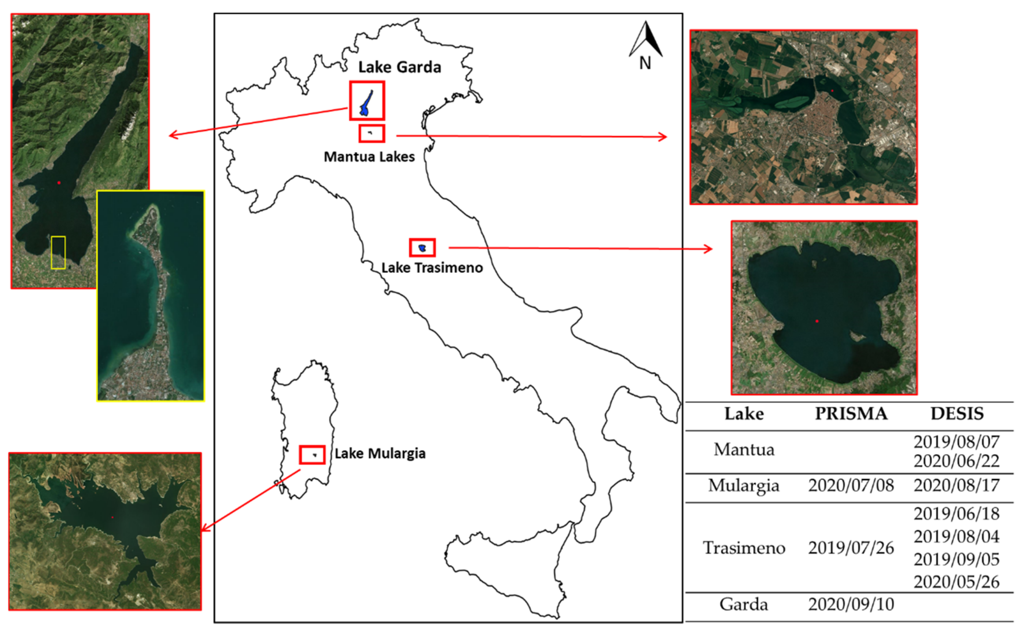
3. Study Area, Imagery Data and Processing
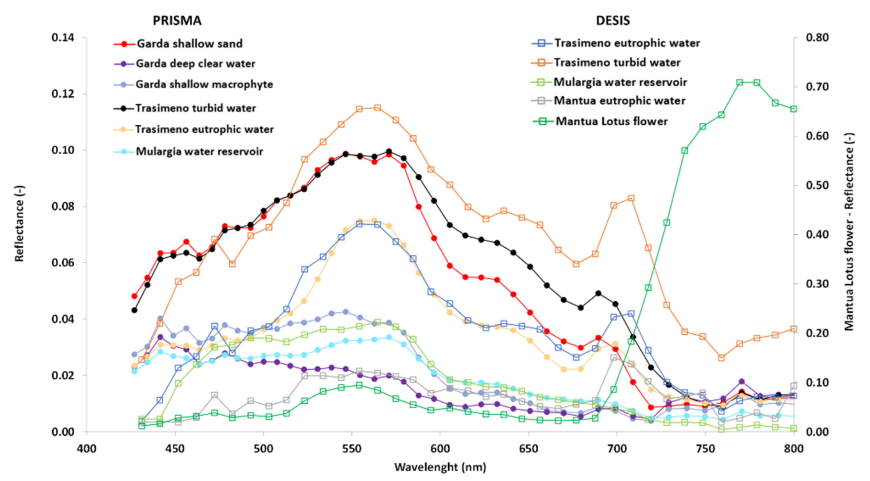
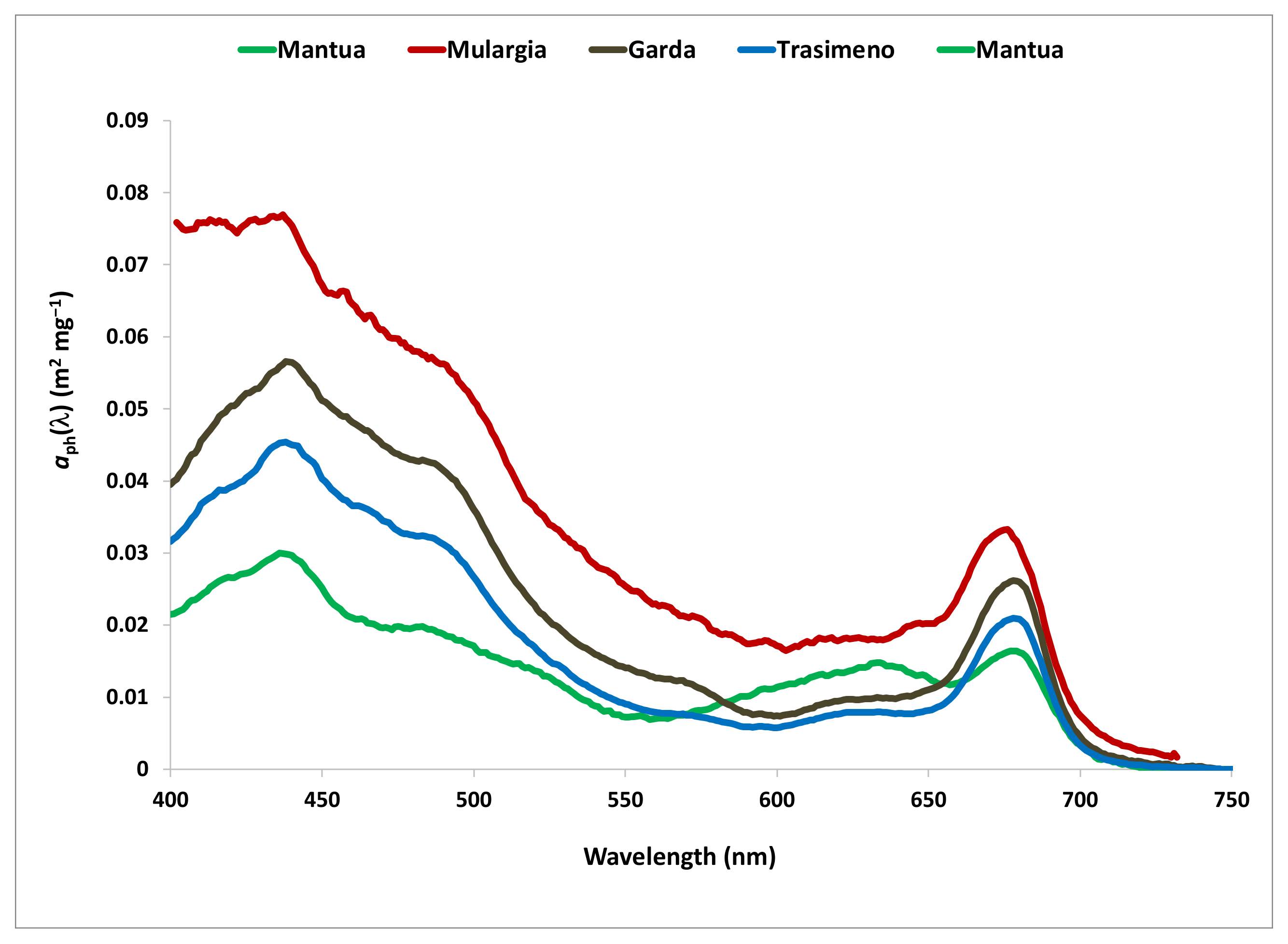
4. Exploitation of PRISMA and DESIS Products for Water Quality Mapping
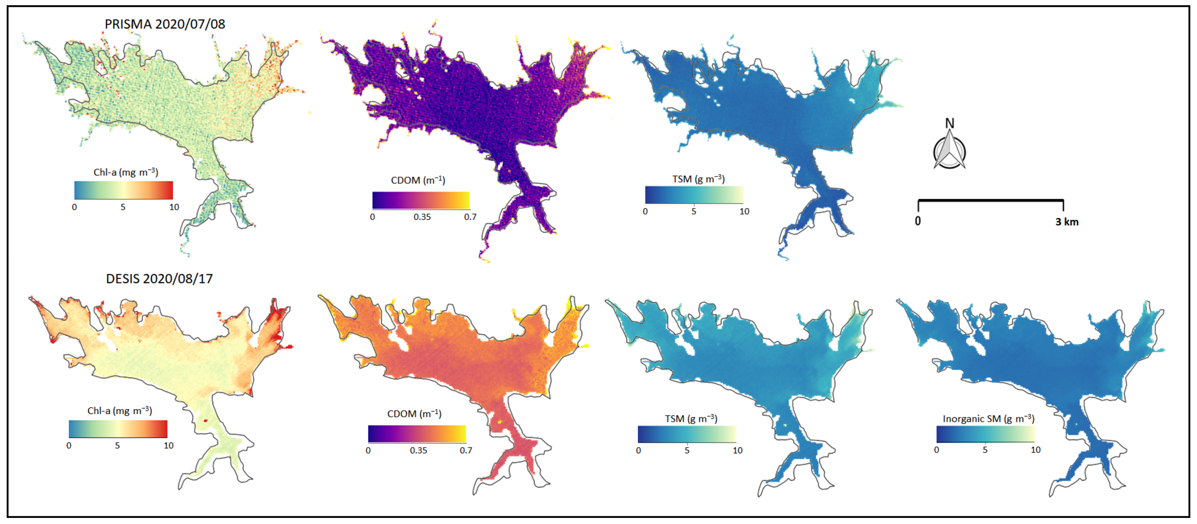
4.1. Mantua Lakes
4.2. Lake Mulargia
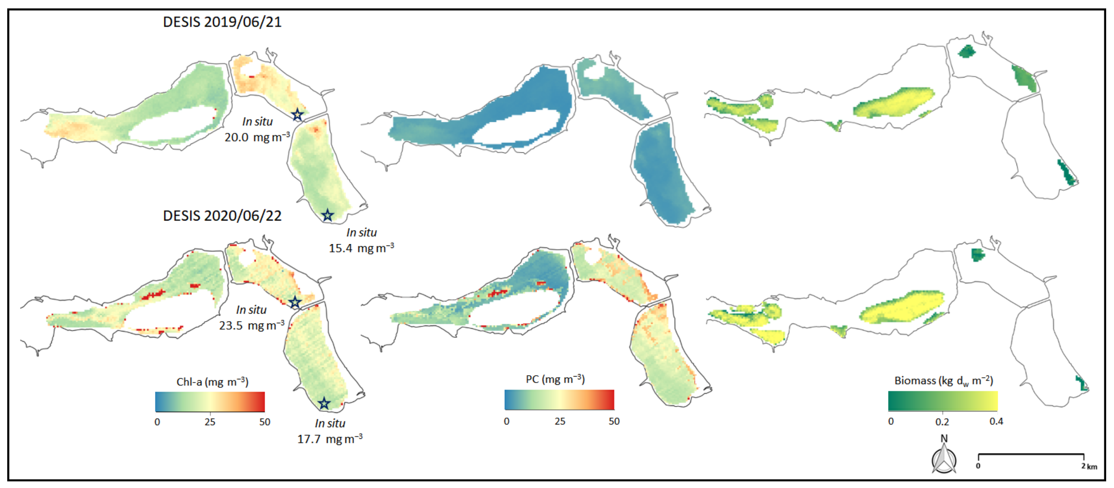
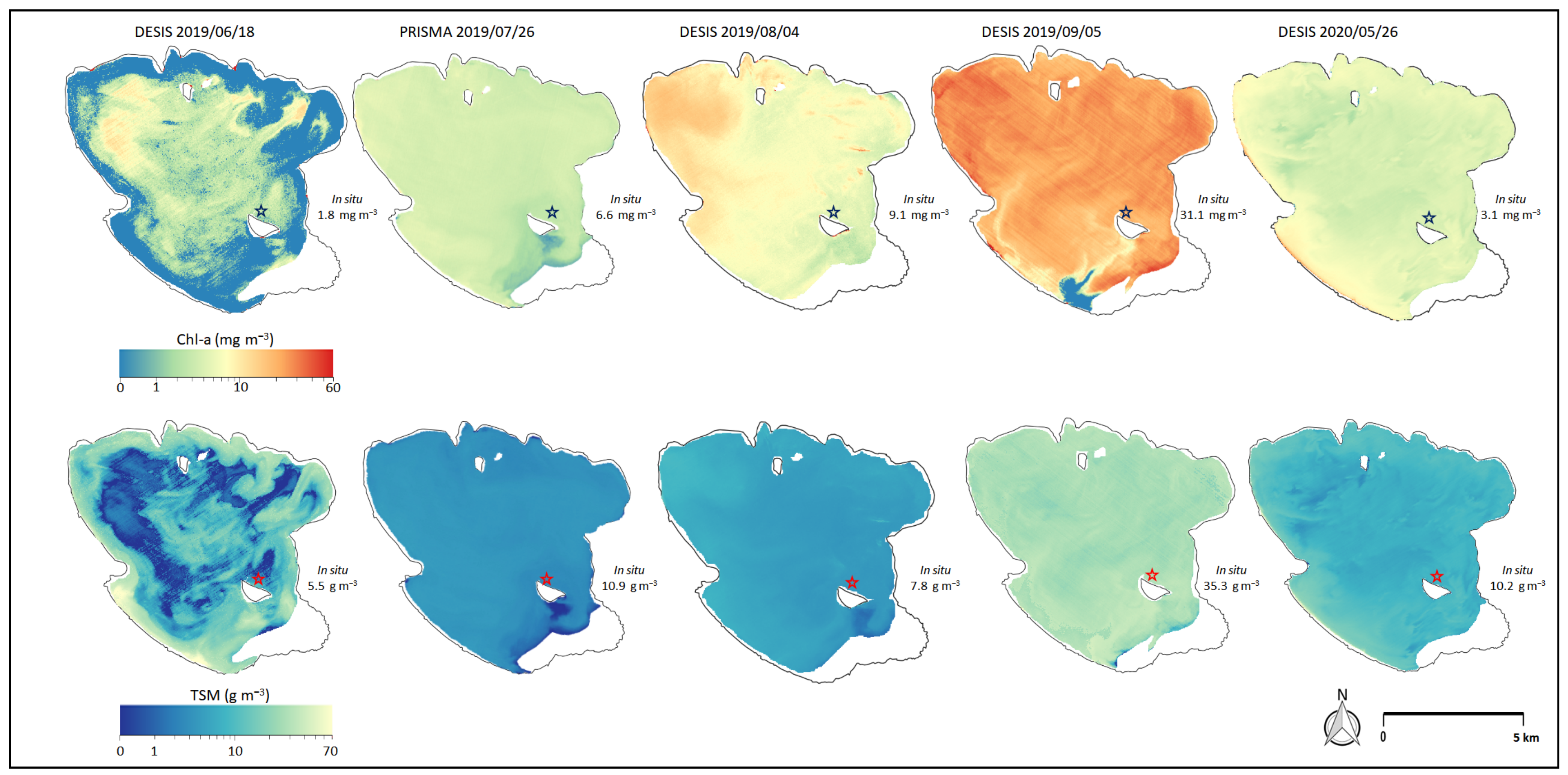
4.3. Lake Trasimeno
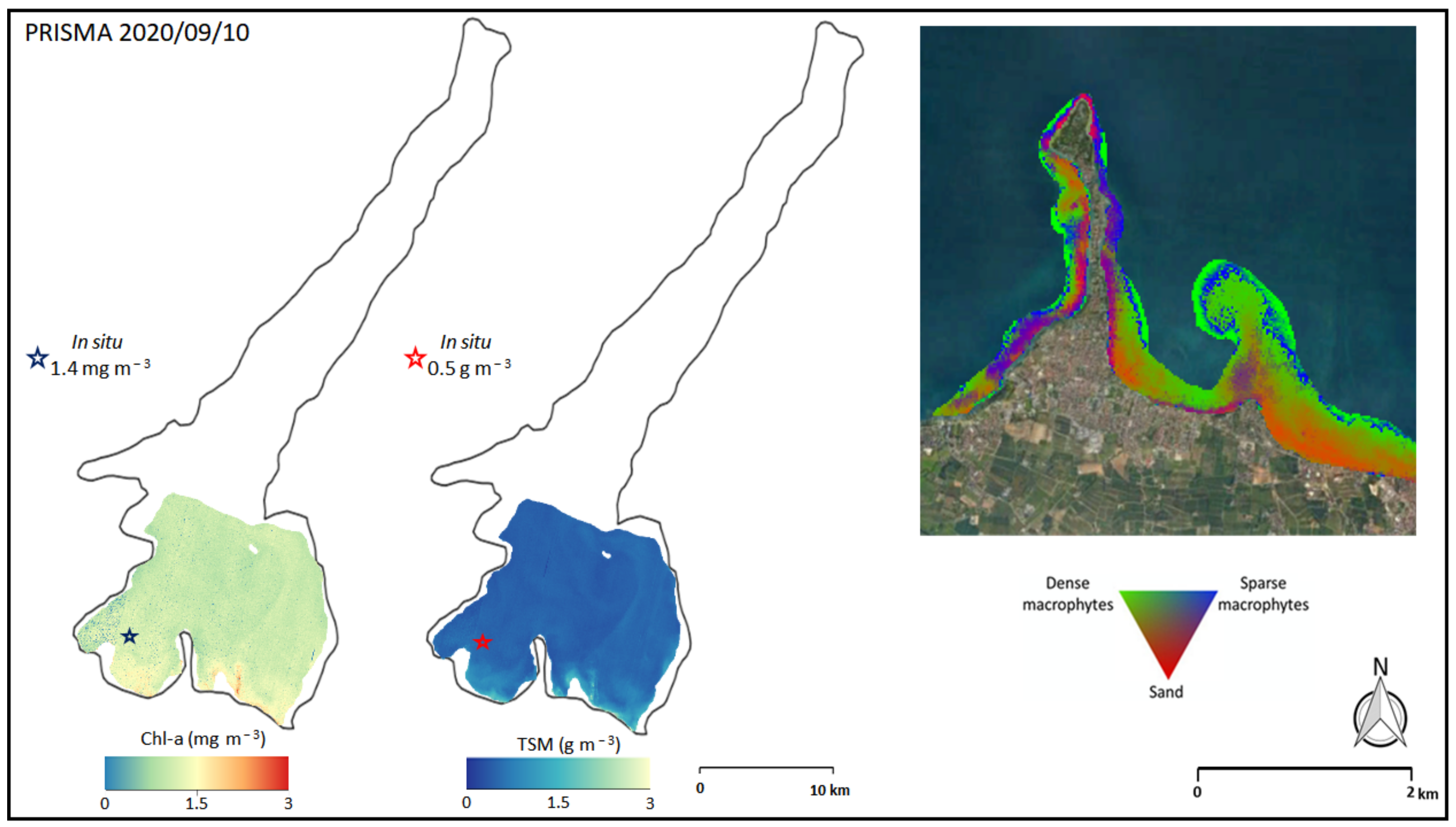
5. Lake Garda
6. Conclusions
Author Contributions
Funding
Institutional Review Board Statement
Informed Consent Statement
Data Availability Statement
Acknowledgments
Conflicts of Interest
References
- Likens, G.E. Lake ecosystem ecology: A global perspective. In Encyclopedia of Inland Waters; Academic Press: Cambridge, MA, USA, 2010. [Google Scholar]
- Hanjra, M.A.; Qureshi, M.E. Global water crisis and future food security in an era of climate change. Food Policy 2010, 35, 365–377. [Google Scholar] [CrossRef]
- Ormerod, S.J.; Dobson, M.; Hildrew, A.G.; Townsend, C.R. Multiple stressors in freshwater ecosystems. Freshw. Biol. 2010, 55, 1–4. [Google Scholar] [CrossRef]
- Carpenter, S.R.; Stanley, E.H.; Vander Zanden, M.J. State of the World’s Freshwater Ecosystems: Physical, Chemical, and Biological Changes. Annu. Rev. Environ. Resour. 2011, 36, 75–99. [Google Scholar] [CrossRef] [Green Version]
- Ho, J.C.; Michalak, A.M.; Pahlevan, N. Widespread global increase in intense lake phytoplankton blooms since the 1980s. Nature 2019, 574, 667–670. [Google Scholar] [CrossRef] [PubMed]
- Visser, P.M.; Verspagen, J.M.; Sandrini, G.; Stal, L.J.; Matthijs, H.C.; Davis, T.W.; Paerl, H.W.; Huisman, J. How rising CO2 and global warming may stimulate harmful cyanobacterial blooms. Harmful Algae 2016, 54, 145–159. [Google Scholar] [CrossRef] [Green Version]
- Carvalho, L.; Mackay, E.B.; Cardoso, A.C.; Baattrup-Pedersen, A.; Birk, S.; Blackstock, K.L.; Borics, G.; Borja, A.; Feld, C.K.; Ferreira, M.T.; et al. Protecting and restoring Europe’s waters: An analysis of the future development needs of the water framework directive. Sci. Total Environ. 2019, 658, 1228–1238. [Google Scholar] [CrossRef]
- Council of the European Communities. Directive 2000/60/EC of the European parliament and of the council of 23 October 2000 establishing a framework for community action in the field of water policy. Off. J. Eur. Communities 2000, 327, 1–72. [Google Scholar]
- European Commission. Commission decision of 20 September 2013 establishing pursuant to directive 2000/60/EC of the European parliament and of the council, the values of the member state monitoring system classifications as a result of the intercalibration exercise and repealing decision 2008/915/EC. Off. J. Eur. Union 2013, 266, 1–47. [Google Scholar]
- Papathanasopoulou, E.; Simis, S.; Alikas, K.; Ansper, A.; Anttila, J.; Barillé, A.; Barillé, L.; Brando, V.; Bresciani, M.; Bučas, M.; et al. Satellite-Assisted Monitoring of Water Quality to Support the Implementation of the Water Framework Directive. EOMORES White Paper; European Union’s Horizon 2020 Project. Available online: https://zenodo.org/record/3903776#.YUDJ8J0zZPY (accessed on 1 November 2021).
- Tyler, A.N.; Hunter, P.D.; Spyrakos, E.; Groom, S.; Constantinescu, A.M.; Kitchen, J. Developments in Earth observation for the assessment and monitoring of inland, transitional, coastal and shelf-sea waters. Sci. Total Environ. 2016, 572, 1307–1321. [Google Scholar] [CrossRef] [Green Version]
- Kiefer, I.; Odermatt, D.; Anneville, O.; Wüest, A.; Bouffard, D. Application of remote sensing for the optimization of in-situ sampling for monitoring of phytoplankton abundance in a large lake. Sci. Total Environ. 2015, 527, 493–506. [Google Scholar] [CrossRef]
- Ritchie, J.C.; Zimba, P.V.; Everitt, J.H. Remote sensing techniques to assess water quality. Photogramm. Eng. Remote Sens. 2003, 69, 695–704. [Google Scholar] [CrossRef] [Green Version]
- Crétaux, J.-F.; Merchant, C.J.; Duguay, C.; Simis, S.; Calmettes, B.; Bergé-Nguyen, M.; Wu, Y.; Zhang, D.; Carrea, L.; Liu, X.; et al. ESA Lakes Climate Change Initiative (Lakes_cci): Lake Products, Version 1.1. 2020. Available online: https://catalogue.ceda.ac.uk/uuid/3c324bb4ee394d0d876fe2e1db217378 (accessed on 1 November 2021).
- Gholizadeh, M.; Melesse, A.; Reddi, L.A. Comprehensive Review on Water Quality Parameters Estimation Using Remote Sensing Techniques. Sensors 2016, 16, 1298. [Google Scholar] [CrossRef] [PubMed] [Green Version]
- Greb, S.; Dekker, A.G.; Binding, C.; Bernard, S.; Brockmann, C.; DiGiacomo, P.; Griffith, D.; Groom, S.; Hestir, E.; Hunter, P.; et al. Earth Observations in Support of Global Water Quality Monitoring; International Ocean-Colour Coordinating Group: Dartmouth, NS, Canada, 2018. [Google Scholar]
- Bresciani, M.; Giardino, C.; Stroppiana, D.; Dessena, M.A.; Buscarinu, P.; Cabras, L.; Schenk, K.; Heege, T.; Bernet, H.; Bazdanis, G.; et al. Monitoring water quality in two dammed reservoirs from multispectral satellite data. Eur. J. Remote Sens. 2019, 52, 113–122. [Google Scholar] [CrossRef]
- Seegers, B.N.; Werdell, P.J.; Vandermeulen, R.A.; Salls, W.; Stumpf, R.P.; Schaeffer, B.A.; Owens, T.J.; Bailey, S.W.; Scott, J.P.; Loftin, K.A. Satellites for long-term monitoring of inland US lakes: The MERIS time series and application for chlorophyll-a. Remote Sens. Environ. 2021, 266, 112685. [Google Scholar] [CrossRef]
- Dekker, A.G.; Hestir, E.L. Evaluating the Feasibility of Systematic Inland Water Quality Monitoring with Satellite Remote Sensing; Commonwealth Scientific and Industrial Research Organization: Canberra, Australia, 2012. [Google Scholar]
- Andres, L.; Boateng, K.; Borja-Vega, C.; Thomas, E. A review of in-situ and remote sensing technologies to monitor water and sanitation interventions. Water 2018, 10, 756. [Google Scholar] [CrossRef] [Green Version]
- Sheffield, J.; Wood, E.F.; Pan, M.; Beck, H.; Coccia, G.; Serrat-Capdevila, A.; Verbist, K. Satellite remote sensing for water resources management: Potential for supporting sustainable development in data-poor regions. Water Resour. Res. 2018, 54, 9724–9758. [Google Scholar] [CrossRef] [Green Version]
- Gómez, J.A.D.; Alonso, C.A.; García, A.A. Remote sensing as a tool for monitoring water quality parameters for Mediterranean Lakes of European Union water framework directive (WFD) and as a system of surveillance of cyanobacterial harmful algae blooms (SCyanoHABs). Environ. Monit. Assess. 2011, 181, 317–334. [Google Scholar] [CrossRef]
- Alikas, K.; Kratzer, S. Improved retrieval of Secchi depth for optically-complex waters using remote sensing data. Ecol. Indic. 2017, 77, 218–227. [Google Scholar] [CrossRef]
- Yigit Avdan, Z.; Kaplan, G.; Goncu, S.; Avdan, U. Monitoring the water quality of small water bodies using high-resolution remote sensing data. ISPRS Int. J. Geo-Inf. 2019, 8, 553. [Google Scholar] [CrossRef] [Green Version]
- Claverie, M.; Ju, J.; Masek, J.G.; Dungan, J.L.; Vermote, E.F.; Roger, J.-C.; Skakun, S.V.; Justice, C. The Harmonized Landsat and Sentinel-2 surface reflectance data set. Remote Sens. Environ. 2018, 219, 145–161. [Google Scholar] [CrossRef]
- Mouw, C.B.; Hardman-Mountford, N.J.; Alvain, S.; Bracher, A.; Brewin, R.; Bricaud, A.; Ciotti, A.M.; Devred, E.; Fujiwara, A.; Hirata, T.; et al. A consumer’s guide to satellite remote sensing of multiple phytoplankton groups in the global ocean. Front. Mar. Sci. 2017, 4, 41. [Google Scholar] [CrossRef] [Green Version]
- Giardino, C.; Brando, V.E.; Gege, P.; Pinnel, N.; Hochberg, E.; Knaeps, E.; Reusen, I.; Doerffer, R.; Bresciani, M.; Braga, F.; et al. Imaging Spectrometry of Inland and Coastal Waters: State of the Art, Achievements and Perspectives. Surv. Geophys. 2019, 40, 401–429. [Google Scholar] [CrossRef] [Green Version]
- Dey, J.; Vijay, R. A critical and intensive review on assessment of water quality parameters through geospatial techniques. Environ. Sci. Pollut. Res. 2021, 28, 41612–41626. [Google Scholar] [CrossRef] [PubMed]
- Pahlevan, N.; Mangin, A.; Balasubramanian, S.V.; Smith, B.; Alikas, K.; Arai, K.; Barbosa, C.; Bélanger, S.; Binding, C.; Bresciani, M.; et al. ACIX-Aqua: A global assessment of atmospheric correction methods for Landsat-8 and Sentinel-2 over lakes, rivers, and coastal waters. Remote Sens. Environ. 2021, 258, 112366. [Google Scholar] [CrossRef]
- Warren, M.A.; Simis, S.G.; Selmes, N. Complementary water quality observations from high and medium resolution Sentinel sensors by aligning chlorophyll-a and turbidity algorithms. Remote Sens. Environ. 2021, 265, 112651. [Google Scholar] [CrossRef] [PubMed]
- Dierssen, H.M.; Ackleson, S.G.; Joyce, K.; Hestir, E.; Castagna, A.; Lavender, S.J.; McManus, M.A. Living up to the Hype of Hyperspectral Aquatic Remote Sensing: Science, Resources and Outlook. Front. Environ. Sci. 2021, 9, 134. [Google Scholar] [CrossRef]
- Palmer, S.C.; Kutser, T.; Hunter, P.D. Remote sensing of inland waters: Challenges, progress and future directions. Remote Sens. Environ. 2015, 157, 1–8. [Google Scholar] [CrossRef] [Green Version]
- Ogashawara, I.; Mishra, D.R.; Gitelson, A.A. Remote sensing of inland waters: Background and current state-of-the-art. In Bio-Optical Modeling and Remote Sensing of Inland Waters; Elsevier: Amsterdam, The Netherlands, 2017; pp. 1–24. [Google Scholar]
- Matthews, M.W. A current review of empirical procedures of remote sensing in Inland and near-coastal transitional waters. Int. J. Remote Sens. 2011, 32, 6855–6899. [Google Scholar] [CrossRef]
- Giardino, C.; Bresciani, M.; Stroppiana, D.; Oggioni, A.; Morabito, G. Optical remote sensing of lakes: An overview on Lake Maggiore. J. Limnol. 2014, 73, 201–214. [Google Scholar] [CrossRef] [Green Version]
- Pu, H.; Liu, D.; Qu, J.H.; Sun, D.W. Applications of imaging spectrometry in inland water quality monitoring—A review of recent developments. Water Air Soil Pollut. 2017, 228, 131. [Google Scholar] [CrossRef]
- Odermatt, D.; Gitelson, A.; Brando, V.E.; Schaepman, M. Review of constituent retrieval in optically deep and complex waters from satellite imagery. Remote Sens. Environ. 2012, 118, 116–126. [Google Scholar] [CrossRef] [Green Version]
- Malthus, T.J.; Lehmann, E.; Ho, X.; Botha, E.; Anstee, J. Implementation of a satellite based inland water algal bloom alerting system using analysis ready data. Remote Sens. 2019, 11, 2954. [Google Scholar] [CrossRef] [Green Version]
- Sagan, V.; Peterson, K.T.; Maimaitijiang, M.; Sidike, P.; Sloan, J.; Greeling, B.A.; Maalouf, S.; Adams, C. Monitoring inland water quality using remote sensing: Potential and limitations of spectral indices, bio-optical simulations, machine learning, and cloud computing. Earth-Sci. Rev. 2020, 205, 103187. [Google Scholar] [CrossRef]
- Topp, S.N.; Pavelsky, T.M.; Jensen, D.; Simard, M.; Ross, M.R. Research trends in the use of remote sensing for inland water quality science: Moving towards multidisciplinary applications. Water 2020, 12, 169. [Google Scholar] [CrossRef] [Green Version]
- Turpie, K.R.; Klemas, V.V.; Byrd, K.; Kelly, M.; Jo, Y.H. Prospective HyspIRI global observations of tidal wetlands. Remote Sens. Environ. 2015, 167, 206–217. [Google Scholar] [CrossRef] [Green Version]
- Chander, S.; Pompapathi, V.; Gujrati, A.; Singh, R.P.; Chaplot, N.; Patel, U.D. Growth of invasive aquatic macrophytes over Tapi river. Int. Arch. Photogramm. Remote Sens. Spat. Inf. Sci. 2018, 5, 829–833. [Google Scholar] [CrossRef] [Green Version]
- Gupana, R.S.; Odermatt, D.; Cesana, I.; Giardino, C.; Nedbal, L.; Damm, A. Remote sensing of sun-induced chlorophyll-a fluorescence in inland and coastal waters: Current state and future prospects. Remote Sens. Environ. 2021, 262, 112482. [Google Scholar] [CrossRef]
- Silva, T.S.; Costa, M.P.; Melack, J.M.; Novo, E.M. Remote sensing of aquatic vegetation: Theory and applications. Environ. Monit. Assess. 2008, 140, 131–145. [Google Scholar] [CrossRef]
- Hestir, E.L.; Brando, V.E.; Bresciani, M.; Giardino, C.; Matta, E.; Villa, P.; Dekker, A.G. Measuring freshwater aquatic ecosystems: The need for a hyperspectral global mapping satellite mission. Remote Sens. Environ. 2015, 167, 181–195. [Google Scholar] [CrossRef] [Green Version]
- Minghelli, A.; Vadakke-Chanat, S.; Chami, M.; Guillaume, M.; Migne, E.; Grillas, P.; Boutron, O. Estimation of Bathymetry and Benthic Habitat Composition from Hyperspectral Remote Sensing Data (BIODIVERSITY) Using a Semi-Analytical Approach. Remote Sens. 2021, 13, 1999. [Google Scholar] [CrossRef]
- Jay, S.; Guillaume, M.; Minghelli, A.; Deville, Y.; Chami, M.; Lafrance, B.; Serfaty, V. Hyperspectral remote sensing of shallow waters: Considering environmental noise and bottom intra-class variability for modeling and inversion of water reflectance. Remote Sens. Environ. 2017, 200, 352–367. [Google Scholar] [CrossRef]
- Sharma, L.K.; Naik, R.; Pandey, P.C. Efficacy of hyperspectral data for monitoring and assessment of wetland ecosystem. In Hyperspectral Remote Sensing; Elsevier: Amsterdam, The Netherlands, 2020; pp. 221–246. [Google Scholar]
- Koponen, S.; Pulliainen, J.; Kallio, K.; Hallikainen, M. Lake water quality classification with airborne hyperspectral spectrometer and simulated MERIS data. Remote Sens. Environ. 2002, 79, 51–59. [Google Scholar] [CrossRef]
- Cogliati, S.; Sarti, F.; Chiarantini, L.; Cosi, M.; Lorusso, R.; Lopinto, E.; Miglietta, F.; Genesio, L.; Guanter, L.; Damm, A.; et al. The PRISMA imaging spectroscopy mission: Overview and first performance analysis. Remote Sens. Environ. 2021, 262, 112499. [Google Scholar] [CrossRef]
- Dekker, A.G.; Phinn, R.; Anstee, J.; Bissett, P.; Brando, V.E.; Casey, B.; Fearns, P.; Hedley, J.; Klonowski, W.; Lee, Z.P.; et al. Intercomparison of shallow water bathymetry, hydro-optics, and benthos mapping techniques in Australian and Caribbean coastal environments. Limnol. Oceanogr. Methods 2011, 9, 396–425. [Google Scholar] [CrossRef] [Green Version]
- Giardino, C.; Candiani, G.; Zilioli, E. Detecting chlorophyll-a in Lake Garda using TOA MERIS radiances. Photogramm. Eng. Remote Sens. 2005, 71, 1045–1051. [Google Scholar] [CrossRef]
- Coppo, P.; Brandani, F.; Faraci, M.; Sarti, F.; Dami, M.; Chiarantini, L.; Ponticelli, B.; Giunti, L.; Fossati, E.; Cosi, M. Leonardo spaceborne infrared payloads for Earth observation: SLSTRs for Copernicus Sentinel 3 and PRISMA hyperspectral camera for PRISMA satellite. Appl. Opt. 2020, 59, 6888–6901. [Google Scholar] [CrossRef]
- Krutz, D.; Müller, R.; Knodt, U.; Günther, B.; Walter, I.; Sebastian, I.; Säuberlich, T.; Reulke, R.; Carmona, E.; Eckardt, A.; et al. The instrument design of the DLR earth sensing imaging spectrometer (DESIS). Sensors 2019, 19, 1622. [Google Scholar] [CrossRef] [PubMed] [Green Version]
- Richter, R.; Schläpfer, D. Atmospheric/Topographic Correction for Satellite Imagery; ATCOR-2/3 User Guide, Version 9.4.0, July 2021. Available online: https://www.rese-apps.com/pdf/atcor3_manual.pdf (accessed on 15 September 2021).
- Pahlevan, N.; Smith, B.; Binding, C.; Gurlin, D.; Li, L.; Bresciani, M.; Giardino, C. Hyperspectral retrievals of phytoplankton absorption and chlorophyll-a in inland and nearshore coastal waters. Remote Sens. Environ. 2021, 253, 112200. [Google Scholar] [CrossRef]
- O’Shea, R.E.; Pahlevan, N.; Smith, B.; Bresciani, M.; Egerton, T.; Giardino, C.; Li, L.; Moore, T.; Ruiz-Verdu, A.; Ruberg, S.; et al. Advancing cyanobacteria biomass estimation from hyperspectral observations: Demonstrations with HICO and PRISMA imagery. Remote Sens. Environ. 2021, 266, 112693. [Google Scholar] [CrossRef]
- Bracher, A.; Soppa, M.A.; Gege, P.; Losa, S.N.; Silva, B.; Steinmetz, F.; Dröscher, I. Extension of Atmospheric Correction Polymer to Hyperspectral Sensors: Application to HICO and First Results for DESIS Data. In Proceedings of the 2021 IEEE International Geoscience and Remote Sensing Symposium—IGARSS, Brussels, Belgium, 11–16 July 2021; pp. 1237–1240. [Google Scholar]
- Lee, Z.; Carder, K.L.; Mobley, C.D.; Steward, R.G.; Patch, J.S. Hypespectral remote sensing for shallow waters: 1. A semianalytical model. Appl. Opt. 1998, 37, 6329–6338. [Google Scholar] [CrossRef]
- Lee, Z.; Carder, K.L.; Chen, R.F.; Peacock, T.G. Properties of the water column and bottom derived from Airborne Visible Infrared Imaging Specrometer (AVIRIS) data. J. Geophys. Res. 2001, 106, 11639–11651. [Google Scholar] [CrossRef] [Green Version]
- Giardino, C.; Candiani, G.; Bresciani, M.; Lee, Z.; Gagliano, S.; Pepe, M. BOMBER: A tool for estimating water quality and bottom properties from remote sensing images. Comput. Geosci. 2012, 45, 313–318. [Google Scholar] [CrossRef]
- Giardino, C.; Bresciani, M.; Cazzaniga, I.; Schenk, K.; Rieger, P.; Braga, F.; Matta, E.; Brando, V.E. Evaluation of multi-resolution satellite sensors for assessing water quality and bottom depth of Lake Garda. Sensors 2014, 14, 24116–24131. [Google Scholar] [CrossRef] [PubMed] [Green Version]
- Giardino, C.; Bresciani, M.; Valentini, E.; Gasperini, L.; Bolpagni, R.; Brando, V.E. Airborne hyperspectral data to assess suspended particulate matter and aquatic vegetation in a shallow and turbid lake. Remote Sens. Environ. 2015, 157, 48–57. [Google Scholar] [CrossRef]
- Babin, M.; Stramski, D.; Ferrari, G.M.; Claustre, H.; Bricaud, A.; Obolensky, G.; Hoepffner, N. Variations in the light absorption coefficients of phytoplankton, nonalgal particles, and dissolved organic matter in coastal waters around Europe. J. Geophys. Res. Ocean. 2003, 108, 3211. [Google Scholar] [CrossRef]
- Blondeau-Patissier, D.; Brando, V.E.; Oubelkheir, K.; Dekker, A.G.; Clementson, L.A.; Daniel, P. Bio-optical variability of the absorption and scattering properties of the Queensland inshore and reef waters, Australia. J. Geophys. Res. Ocean. 2009, 114, C05003. [Google Scholar] [CrossRef]
- Kallio, K. Optical properties of Finnish lakes estimated with simple bio-optical models and water quality monitoring data. Hydrol. Res. 2006, 37, 183–204. [Google Scholar] [CrossRef]
- Ghirardi, N.; Bolpagni, R.; Bresciani, M.; Valerio, G.; Pilotti, M.; Giardino, C. Spatiotemporal dynamics of submerged aquatic vegetation in a deep lake from Sentinel-2 data. Water 2019, 11, 563. [Google Scholar] [CrossRef] [Green Version]
- Villa, P.; Pinardi, M.; Tóth, V.R.; Hunter, P.D.; Bolpagni, R.; Bresciani, M. Remote sensing of macrophyte morphological traits: Implications for the management of shallow lakes. J. Limnol. 2017, 76, 109–126. [Google Scholar] [CrossRef] [Green Version]
- Pinardi, M.; Fenocchi, A.; Giardino, C.; Sibilla, S.; Bartoli, M.; Bresciani, M. Assessing potential algal blooms in shallow fluvial lake by combining hydrodynamic modelling and remote-sensed images. Water 2015, 7, 1921–1942. [Google Scholar] [CrossRef] [Green Version]
- Pinardi, M.; Soana, E.; Laini, A.; Bresciani, M.; Bartoli, M. Soil system budgets of N, Si and P in an agricultural irrigated watershed: Surplus, differential export and underlying mechanisms. Biogeochemistry 2018, 140, 175–197. [Google Scholar] [CrossRef]
- Pinardi, M.; Soana, E.; Bresciani, M.; Villa, P.; Bartoli, M. Upscaling nitrogen removal processes in fluvial wetlands and irrigation canals in a patchy agricultural watershed. Wetl. Ecol. Manag. 2020, 28, 297–313. [Google Scholar] [CrossRef]
- Bolpagni, R.; Bresciani, M.; Laini, A.; Pinardi, M.; Matta, E.; Ampe, E.M.; Giardino, C.; Viaroli, P.; Bartoli, M. Remote sensing of phytoplankton-macrophyte coexistence in shallow hypereutrophic fluvial lakes. Hydrobiologia 2014, 737, 67–76. [Google Scholar] [CrossRef]
- Bresciani, M.; Rossini, M.; Morabito, G.; Matta, E.; Pinardi, M.; Cogliati, S.; Julitta, T.; Colombo, R.; Braga, F.; Giardino, C. Analysis of within-and between-day chlorophyll-a dynamics in Mantua Superior Lake, with a continuous spectroradiometric measurement. Mar. Freshw. Res. 2013, 64, 303–316. [Google Scholar] [CrossRef]
- Pinardi, M.; Bresciani, M.; Villa, P.; Cazzaniga, I.; Laini, A.; Tóth, V.; Fadel, A.; Austoni, M.; Lami, A.; Giardino, C. Spatial and temporal dynamics of primary producers in shallow lakes as seen from space: Intra-annual observations from Sentinel-2A. Limnologica 2018, 72, 32–43. [Google Scholar] [CrossRef]
- Pinardi, M.; Bartoli, M.; Longhi, D.; Viaroli, P. Net autotrophy in a fluvial lake: The relative role of phytoplankton and floating-leaved macrophytes. Aquat. Sci. 2011, 73, 389–403. [Google Scholar] [CrossRef]
- Pinardi, M.; Free, G.; Lotto, B.; Ghirardi, N.; Bartoli, M.; Bresciani, M. Exploiting high frequency monitoring and satellite imagery for assessing chlorophyll-a dynamics in a shallow eutrophic lake. J. Limnol. 2021, 80. [Google Scholar] [CrossRef]
- Bresciani, M.; Giardino, C.; Lauceri, R.; Matta, E.; Cazzaniga, I.; Pinardi, M.; Lami, A.; Austoni, M.; Viaggiu, E.; Congestri, R.; et al. Earth observation for monitoring and mapping of cyanobacteria blooms. Case studies on five Italian lakes. J. Limnol. 2017, 76, 127–139. [Google Scholar] [CrossRef] [Green Version]
- Villa, P.; Bresciani, M.; Bolpagni, R.; Pinardi, M.; Giardino, C. A rule-based approach for mapping macrophyte communities using multi-temporal aquatic vegetation indices. Remote Sens. Environ. 2015, 171, 218–233. [Google Scholar] [CrossRef] [Green Version]
- Villa, P.; Pinardi, M.; Bolpagni, R.; Gillier, J.M.; Zinke, P.; Nedelcuţ, F.; Bresciani, M. Assessing macrophyte seasonal dynamics using dense time series of medium resolution satellite data. Remote Sens. Environ. 2018, 216, 230–244. [Google Scholar] [CrossRef]
- Bresciani, M.; Giardino, C.; Longhi, D.; Pinardi, M.; Bartoli, M.; Vascellari, M. Imaging spectrometry of productive inland waters. Application to the lakes of Mantua. Ital. J. Remote Sens. 2009, 41, 147–156. [Google Scholar] [CrossRef]
- Ludovisi, A.; Gaino, E. Meteorological and water quality changes in Lake Trasimeno (Umbria, Italy) during the last fifty years. J. Limnol. 2010, 69, 174–188. [Google Scholar] [CrossRef] [Green Version]
- Giardino, C.; Bresciani, M.; Villa, P.; Martinelli, A. Application of Remote Sensing in Water Resource Management: The Case Study of Lake Trasimeno, Italy. Water Resour. Manag. 2010, 24, 3885–3899. [Google Scholar] [CrossRef]
- Charavgis, F.; Cingolani, A.; Di Brizio, M.; Rinaldi, E.; Tozzi, G.; Stranieri, P. Qualita’ Delle Acque Di Balneazione Dei Laghi Umbri, Stagione Balneare 2019; ARPA: Umbria, Italy, 2020. [Google Scholar]
- Bresciani, M.; Pinardi, M.; Free, G.; Luciani, G.; Ghebrehiwot, S.; Laanen, M.; Peters, S.; Della Bella, V.; Padula, R.; Giardino, C. The Use of Multisource Optical Sensors to Study Phytoplankton Spatio-Temporal Variation in a Shallow Turbid Lake. Water 2020, 12, 284. [Google Scholar] [CrossRef] [Green Version]
- Reynolds, C.S. Ecology of Phytoplankton; Cambridge University Press: Cambridge, UK, 2006. [Google Scholar]
- Woods, T.; Kaz, A.; Giam, X. Phenology in freshwaters: A review and recommendations for future research. Ecography 2021, 44, 1–14. [Google Scholar] [CrossRef]
- Free, G.; Bresciani, M.; Pinardi, M.; Giardino, C.; Alikas, K.; Kangro, K.; Rõõm, E.-I.; Vaičiūtė, D.; Bučas, M.; Tiškus, E.; et al. Detecting Climate Driven Changes in Chlorophyll-a Using High Frequency Monitoring: The Impact of the 2019 European Heatwave in Three Contrasting Aquatic Systems. Sensors 2021, 21, 6242. [Google Scholar] [CrossRef]
- Dörnhöfer, K.; Klinger, P.; Heege, T.; Oppelt, N. Multi-sensor satellite and in situ monitoring of phytoplankton development in a eutrophic-mesotrophic lake. Sci. Total Environ. 2018, 612, 1200–1214. [Google Scholar] [CrossRef]
- Arabi, B.; Salama, M.S.; Pitarch, J.; Verhoef, W. Integration of in-situ and multi-sensor satellite observations for long-term water quality monitoring in coastal areas. Remote Sens. Environ. 2020, 239, 111632. [Google Scholar] [CrossRef]
- Bresciani, M.; Giardino, C.; Boschetti, L. Multi-temporal assessment of bio-physical parameters in lakes Garda and Trasimeno from MODIS and MERIS. Ital. J. Remote Sens. Riv. Ital. Telerilevamento 2011, 43, 49–62. [Google Scholar]
- Niroumand-Jadidi, M.; Bovolo, F.; Bruzzone, L. Water Quality Retrieval from PRISMA Hyperspectral Images: First Experience in a Turbid Lake and Comparison with Sentinel-2. Remote Sens. 2020, 12, 3984. [Google Scholar] [CrossRef]
- Hinegk, L.; Adami, L.; Zolezzi, G.; Tubino, M. Implications of water resources management on the long-term regime of Lake Garda (Italy). J. Environ. Manag. 2022, 301, 113893. [Google Scholar] [CrossRef]
- Salmaso, N.; Mosello, R. Limnological research in the deep southern subalpine lakes: Synthesis, directions and perspectives. Adv. Oceanogr. Limnol. 2010, 1, 29–66. [Google Scholar] [CrossRef]
- Salmaso, N. Long-term phytoplankton community changes in a deep subalpine lake: Responses to nutrient availability and climatic fluctuations. Freshw. Biol. 2010, 55, 825–846. [Google Scholar] [CrossRef]
- Bresciani, M.; Bolpagni, R.; Braga, F.; Oggioni, A.; Giardino, C. Retrospective assessment of macrophytic communities in southern Lake Garda (Italy) from in situ and MIVIS (Multispectral Infrared and Visible Imaging Spectrometer) data. J. Limnol. 2012, 71, 180–190. [Google Scholar] [CrossRef] [Green Version]
- Giardino, C.; Bartoli, M.; Candiani, G.; Bresciani, M.; Pellegrini, L. Recent changes in macrophyte colonisation patterns: An imaging spectrometry-based evaluation of southern Lake Garda (northern Italy). J. Appl. Remote Sens. 2007, 1, 011509. [Google Scholar]
- Brivio, P.A.; Giardino, C.; Zilioli, E. Determination of chlorophyll concentration changes in Lake Garda using an image-based radiative transfer code for Landsat TM images. Int. J. Remote Sens. 2001, 22, 487–502. [Google Scholar] [CrossRef]
- Giardino, C.; Brando, V.E.; Dekker, A.G.; Strömbeck, N.; Candiani, G. Assessment of water quality in Lake Garda (Italy) using Hyperion. Remote Sens. Environ. 2007, 109, 183–195. [Google Scholar] [CrossRef]
- Bresciani, M.; Stroppiana, D.; Odermatt, D.; Morabito, G.; Giardino, C. Assessing remotely sensed chlorophyll-a for the implementation of the water framework directive in European perialpine lakes. Sci. Total Environ. 2011, 409, 3083–3091. [Google Scholar] [CrossRef] [PubMed] [Green Version]
- Di Nicolantonio, W.; Cazzaniga, I.; Cacciari, A.; Bresciani, M.; Giardino, C. Synergy of multispectral and multisensors satellite observations to evaluate desert aerosol transport and impact of dust deposition on inland waters: Study case of Lake Garda. J. Appl. Remote Sens. 2015, 9, 095980. [Google Scholar] [CrossRef] [Green Version]
- Ghirardi, N.; Amadori, M.; Free, G.; Giovannini, L.; Toffolon, M.; Giardino, C.; Bresciani, M. Using remote sensing and numerical modelling to quantify a turbidity discharge event in Lake Garda. J. Limnol. 2021, 80, 47–52.6p. [Google Scholar] [CrossRef]
- Dekker, A.; Committee on Earth Observation Satellites (CEOS). Feasibility Study for an Aquatic Ecosystem Earth Observing System. 2021. Available online: https://ceos.org/ (accessed on 15 September 2021).
- Müller, R.; Avbelj, J.; Carmona, E.; Gerasch, B.; Graham, L.; Günther, B.; Heiden, U.; Kerr, G.; Knodt, U.; Krutz, D.; et al. The new hyperspectral sensor DESIS on the multi-payload platform MUSES installed on the ISS. Int. Arch. Photogramm. Remote Sens. Spat. Inf. Sci. 2016, 41, 461–467. [Google Scholar] [CrossRef] [Green Version]
- Liu, S.; Marinelli, D.; Bruzzone, L.; Bovolo, F. A review of change detection in multitemporal hyperspectral images: Current techniques, applications, and challenges. IEEE Geosci. Remote Sens. Mag. 2019, 7, 140–158. [Google Scholar] [CrossRef]
- Ren, K.; Sun, W.; Meng, X.; Yang, G.; Du, Q. Fusing China GF-5 Hyperspectral Data with GF-1, GF-2 and Sentinel-2A Multispectral Data: Which Methods Should Be Used? Remote Sens. 2020, 12, 882. [Google Scholar] [CrossRef] [Green Version]
- Bachmann, M.; Alonso, K.; Carmona, E.; Gerasch, B.; Habermeyer, M.; Holzwarth, S.; Krawczyk, H.; Langheinrich, M.; Marshall, D.; Pato, M.; et al. Analysis-Ready Data from Hyperspectral Sensors—The Design of the EnMAP CARD4L-SR Data Product. Remote Sens. 2021, 13, 4536. [Google Scholar] [CrossRef]
- Rast, M.; Nieke, J.; Adams, J.; Isola, C.; Gascon, F. Copernicus Hyperspectral Imaging Mission for the Environment (Chime). In Proceedings of the 2021 IEEE International Geoscience and Remote Sensing Symposium—IGARSS, Brussels, Belgium, 12–16 July 2021; pp. 108–111. [Google Scholar]
- Seifert-Dähnn, I.; Furuseth, I.S.; Vondolia, G.K.; Gal, G.; de Eyto, E.; Jennings, E.; Pierson, D. Costs and Benefits of Automated High-Frequency Environmental Monitoring—The Case of Lake Water Management. J. Environ. Manag. 2021, 285, 112108. [Google Scholar] [CrossRef]
- Goffi, G.; Osti, L.; Nava, C.R.; Maurer, O.; Pencarelli, T. Is Preservation the Key to Quality and Tourists’ Satisfaction? Evidence from Lake Garda. Tour. Recreat. Res. 2021, 46, 434–440. [Google Scholar] [CrossRef]
- Guanter, L.; Brell, M.; Chan, J.C.W.; Giardino, C.; Gomez-Dans, J.; Mielke, C.; Morsdorf, F.; Segl, K.; Yokoya, N. Synergies of spaceborne imaging spectroscopy with other remote sensing approaches. Surv. Geophys. 2019, 40, 657–687. [Google Scholar] [CrossRef]
- Taramelli, A.; Tornato, A.; Magliozzi, M.L.; Mariani, S.; Valentini, E.; Zavagli, M.; Costantini, M.; Nieke, J.; Adams, J.; Rast, M. An interaction methodology to collect and assess user-driven requirements to define potential opportunities of future hyperspectral imaging sentinel mission. Remote Sens. 2020, 12, 1286. [Google Scholar] [CrossRef] [Green Version]


| PRISMA | DESIS | |
|---|---|---|
| Launch | 22 March 2019 | 29 June 2018 |
| Coverage | 70° N to 70° S | 55° N to 52° S |
| Target lifetime | 5 years | 2018–2023 |
| Orbit | SSO 615 km 10:30 LTDN | MUSES platform on ISS |
| Number of bands | VNIR: 66 (440–1010 nm), SWIR: 174 (920–2505 nm), PAN: 1 (400–700 nm) | 235 (no binning), 60 (binning 4) |
| Spectral sampling interval | VNIR: 7.2–11 nm, SWIR: 6.5–11 nm | 2.55 nm (no binning), 10.2 nm (binning 4) |
| Spectral coverage | 440 nm to 2505 nm | 402 nm to 1000 nm |
| Ground sampling distance | Hyperspectral: 30 m, PAN: 5 m | 30 m |
| Signal-to-noise ratio | >160:1 VNIR, >100:1 SWIR, >240:1 PAN | 195 (w/o binning), 386 (4 binning) (based on laboratory calibration) (albedo 0.3 @ 550 nm) |
| Radiometric resolution | 12 bits | 13 bits + 1 bit gain |
| Swath | 30 km | 30 km |
| Parameter | Garda | Mantua | Mulargia | Trasimeno |
|---|---|---|---|---|
| Spectral slope coefficient of CDOM absorption | 0.021 | 0.014 | 0.018 | 0.016 |
| Specific absorption of NAP at 440 nm | 0.05 | 0.30 | 0.11 | 0.20 |
| Spectral slope coefficient of NAP absorption | 0.012 | 0.008 | 0.012 | 0.013 |
| Backscattering exponent of TSM | 0.76 | 0.80 | 0.71 | 0.65 |
| Specific back-scattering coefficient of TSM at 555 nm | 0.0071 | 0.0111 | 0.0105 | 0.0119 |
Publisher’s Note: MDPI stays neutral with regard to jurisdictional claims in published maps and institutional affiliations. |
© 2022 by the authors. Licensee MDPI, Basel, Switzerland. This article is an open access article distributed under the terms and conditions of the Creative Commons Attribution (CC BY) license (https://creativecommons.org/licenses/by/4.0/).
Share and Cite
Bresciani, M.; Giardino, C.; Fabbretto, A.; Pellegrino, A.; Mangano, S.; Free, G.; Pinardi, M. Application of New Hyperspectral Sensors in the Remote Sensing of Aquatic Ecosystem Health: Exploiting PRISMA and DESIS for Four Italian Lakes. Resources 2022, 11, 8. https://0-doi-org.brum.beds.ac.uk/10.3390/resources11020008
Bresciani M, Giardino C, Fabbretto A, Pellegrino A, Mangano S, Free G, Pinardi M. Application of New Hyperspectral Sensors in the Remote Sensing of Aquatic Ecosystem Health: Exploiting PRISMA and DESIS for Four Italian Lakes. Resources. 2022; 11(2):8. https://0-doi-org.brum.beds.ac.uk/10.3390/resources11020008
Chicago/Turabian StyleBresciani, Mariano, Claudia Giardino, Alice Fabbretto, Andrea Pellegrino, Salvatore Mangano, Gary Free, and Monica Pinardi. 2022. "Application of New Hyperspectral Sensors in the Remote Sensing of Aquatic Ecosystem Health: Exploiting PRISMA and DESIS for Four Italian Lakes" Resources 11, no. 2: 8. https://0-doi-org.brum.beds.ac.uk/10.3390/resources11020008