Using KNN Algorithm Predictor for Data Synchronization of Ultra-Tight GNSS/INS Integration

Abstract

The INS system’s update rate is faster than that of the GNSS receiver. Additionally, GNSS receiver data may suffer from blocking for a few seconds for different reasons, affecting architecture integrations between GNSS and INS. This paper proposes a novel GNSS data prediction method using the k nearest neighbor (KNN) predictor algorithm to treat data synchronization between the INS sensors and GNSS receiver and overcome those GNSS receiver’s blocking, which may occur for a few seconds. The experimental work was conducted on a flying drone over a minor Hungarian (Mátyásföld, 47.4992 N, 19.1977 E) model airfield. The GNSS data are predicted by four different scenarios: the first is no blocking of data, and the other three have blocking periods of 1, 4, and 8 s, respectively. Ultra-tight architecture integration is used to perform the GNSS/INS integration to deal with the INS sensors’ inaccuracy and their divergence throughout the operation. The results show that using the GNSS/INS integration system yields better positioning data (in three axes (X, Y, and Z)) than using a stand-alone INS system or GNSS without a predictor.

1. Introduction

The GNSS/INS (Global Navigation Satellite System and Inertial Navigation System) integrates an excellent navigation mechanism due to the INS’s short-term accuracy when it interacts with the GNSS’s long-term accuracy [1]. The INS is a self-contained system that can measure a vehicle’s position, velocity, and attitude with reasonable short-term navigation accuracy. However, as the inertial measurement unit (IMU) veers, the INS navigation error exponentially increases in time, resulting in reduced navigation accuracy [2]. INS continuously calculates position, velocity, and attitude angles during GNSS signal loss for any reason. The main benefits of GNSS against INS are that GNSS globally operates and has higher data precision in all weather conditions. The GNSS, on the other hand, has a lower update rate than the INS, and the satellite signal can be lost or fragmented due to environmental circumstances, including mountains, high buildings, tunnels, and multi-path reflections [3,4].

GNSS has highly accurate guidance information, and INS has a continuously high update rate. These advantages of both stand-alone systems are merged. There are drawbacks as well, such as GNSS measurement’s low update rate, the possibility of absence signal, and the IMU’s drift characteristics in the INS. These drawbacks of both individual frameworks are addressed via the integration synthesis of GNSS/INS. So far, integration of the GNSS/INS framework has been usually established to determine the vehicle’s position and attitude, which can be implemented by using a Kalman filter [5,6,7,8,9].

The GNSS/INS integration systems can be classified into tightly coupled (TC) and ultra-tightly coupled (UTC) integration architectures. The carrier tracking loops in (TC and LC) integration have a large enough bandwidth to retain tracking in the vicinity of drone manoeuvers. Data from the integrated navigation solution are fed back to the GNSS receiver in UTC integration to assist the carrier tracking loops. That results in decreasing the bandwidth of the carrier tracking loops, and, at the same time, it increases the signal-to-noise ratio (SNR) at the output of tracking loops, which leads to more immune systems against jamming and interference [10,11,12].

The problem in all the integration architectures mentioned above is that the INS data rate is higher than the GNSS data rate. Consequently, a predictor should be used to predict the in-between sampling instants of the GNSS receiver in order to synchronize with INS data before the integration process and overcome the GNSS receiver’s stopping time (blocking data) when the signal is lost for a few seconds [12]. Hence, the prediction process benefits two important solutions: first, it gives a high GNSS data rate, and second, it overcomes the problems of GNSS lost signal.

Different prediction algorithms are used in the output of the GNSS or GPS receivers before integration with the INS data for synchronization purposes. In Reference [13], a method proposed to predict GPS data was shown by using a Normalized Least-Mean-Square (NLMS) algorithm. A different blocking time of GPS is taken to show the ability of the algorithms for GPS prediction data. In Reference [14], a comparison between the performance of Radial Basis Function Neural Networks (RBFNN) and Wavelet Neural Networks (WNNs) for GPS data prediction is presented. The results in this paper show that WNNs are more efficient than RBFNNs. Additionally, a carrier phase prediction method on baseband signal processing level to solve GNSS blocking signals in challenging environments was proposed in Reference [15].

Thus, the appropriate selection of the most effective algorithms depends on the purpose of the used technique and its adaptation. In this paper, the k nearest neighbor (KNN) predictor algorithm is used to predict in between sampling instants of GNSS receiver data based on actual GNSS data attributes. The KNN method uses the database to search for data that is similar to the current data. The obtained data are the so-called nearest neighbors of the current data. For the neighborhood classification, a KNN algorithm variant is used. In the case of KNN, when the k parameter is selected, various dataset properties need to be considered. The classification performance is a better choice of a bigger k value, as the effect of noise reduction, but at the same time, the classes will be closer to each other. Thus, the boundaries between the classes are less clear. KNN is a supervised learning algorithm where the training samples determine the classification rules without additional parameters [16]. KNN predicts the new GNSS data points based on the k training samples, which correspond to the measured GNSS data, and the output of the predictor is integrated with the INS data. The whole system is tested on data recorded with a real moving drone at the Mátyásföld airfield. Figure 1 represents the 3D trajectory of the moving drone.

2. Mathematical Models for GNSS/INS Integration

GNSS/INS integration’s main idea is to use the position information measured by GNSS to correct the INS drift errors [12].

The KNN predictor algorithm is used at the GNSS receiver’s output to predict between samples instant of GNSS data for the synchronization purpose with INS.

2.1. K Nearest Neighbor (KNN) Predictor Algorithm

This algorithm’s goal is to predict new GNSS data based on actual GNSS data characteristics. The position information is provided at 1Hz by the GNSS receiver. However, the system which integrates GNSS and INS measurements (see Figure 2) needs the information at 10 Hz. To fulfill this requirement, the predictor will estimate nine new data points at every measured point (for example, for a GNSS measurement at t = 6 s, the predictor provides data to t = 6.1, 6.2, … 6.9 s). If the GNSS receiver is blocked, the predictor will produce estimates for a few seconds. The predictor needs four data points to produce the estimates. For example, at t = 6.1 s, these four preceding points are used for the estimation: t = 5.7, 5.8, 5.9, and 6 s.

The Euclidean distance between real GNSS data (testing data ($x_{\mathrm{test}}$)), and training data ($x_{\mathrm{train}}$) is used in k nearest neighbor to compare the given testing data to training data; one of the similarity measures used is the Euclidean distance between testing data ($x_{\mathrm{test}}$) and training data ($x_{\mathrm{train}}$), as shown in Equation (1) [17]:

$$d\left(X,Y,Z\right)=\sqrt{{\displaystyle \sum }_{i=1}^n{\left(X1-X2\right)}^2+{\displaystyle \sum }_{i=1}^n{\left(Y1-Y2\right)}^2+{\displaystyle \sum }_{i=1}^n{\left(Z1-Z2\right)}^2}$$

(1)

where $x_{\mathrm{train}}$ is X1, Y1, and Z1; and $x_{\mathrm{test}}$ is X2, Y2, and Z2.

The KNN method selects the data points close to the testing data in GNSS ask training data. Hence, the data output from the k training can be chosen to be the nearest neighbors to predict the unknown data of GNSS. Thus, the following KNN equation is used to predict the required data [18]:

$$\widehat{y_l}=\frac{1}{k}{\displaystyle \sum }_{j=1}^k{y}_j$$

(2)

where k is the number of nearest neighbors of y_j.

Hence, to consider the correlation between times, the following equation can be used for GNSS data prediction [17]:

$$\widehat{y_l}= {\displaystyle \sum }_{j=1}^k{\omega }_j{y}_j$$

(3)

where $\widehat{y_l}$ is the testing of the predicted data, ${\omega }_j$ is the weight of the J-neighbor, and $y_j$ is the testing data. Moreover, the number of the training data (n) can be given as follows [17]:

$${\omega }_j=j/n$$

(4)

2.2. Kalman Filter (KF)

For navigation with an INS and GNSS, the INS is the essential keeper of short-term navigation information. The Kalman filter keeps that navigation information as accurate as the noise sources will allow. In GNSS/INS integration, the Kalman filter replaces the stochastic model for unpredictable host vehicle dynamics with the one for the INS and uses it to estimate, correct, and compensate for errors in the INS implementation. A key feature of the integrated navigator is maintaining short-term accuracy when GNSS signals are not available for a few seconds [19,20].

The Kalman filter is the optimal estimator of the expected value of the state of the process in the case of zero-mean white Gaussian noise of the measurements. It is a set of equations in a quadratic form, and the process can be described with a stochastic difference equation [21].

Regardless of any optimum criterion, the Kalman filter is considered the conditional expectation process of the state-space of concern to the whole past observation stream. Thus, the estimated value of X (k) (discrete-time from) is $\widehat{X}\left(k/k\right)$ and defined by [19,22]:

$$\widehat{X}\left(k\right)=E\left\{X\left(k\right)/Y\left(k\right)\right\}$$

(5)

where $\widehat{X}\left(k\right)$ is the estimated state, $E\{ \}$ is the expected value, $Y\left(k\right)$ represents all the data history $\left\{ Y\left(0\right), Y\left(1\right), Y\left(2\right),Y\left(3\right) \dots Y\left(k\right)\right\}$, and the associated estimate error covariance matrix is given by the following:

$$P\left(k/k\right)=E\{[X\left(k\right)-\widehat{X}(k/k)]{[X\left(k\right)-\widehat{X}\left(k/k\right)]}^T\}$$

(6)

where $P\left(k/k\right)$ is the error covariance matrix. The following linear recursive formulas summarize the optimal Kalman filtering algorithm:

• Filter estimate

  $$\begin{array}{c}\widehat{X}\left(k/k\right)=F\left(k,k-1\right)\widehat{X}\left(k-1/k-1\right) +K\left(k\right)[Y\left(k\right)\\ -H\left(k\right)F\left(k,k-1\right)\widehat{X}\left(k-1/k-1\right)]\end{array}$$

  (7)
• Filter gain

  $$K\left(k\right)=P\left(k/k-1\right)H^T\left(k\right){[H\left(k\right)P\left(k/k-1\right)H^T\left(k\right)+R\left(k\right)]}^{-1}$$

  (8)
• Error covariance

  $$P\left(k+1/k\right)=F\left(k,k-1\right)P\left(k/k\right)F^T\left(k,k-1\right)+Q\left(k\right)$$

  (9)

  $$P\left(k/k\right)=\left[I-K\left(k\right)H\left(k\right)\right]P\left(k/k-1\right)$$

  (10)

  where

  $$\hat{X}\left(k\right): n \times 1 \mathrm{estimated} \mathrm{state} \mathrm{vector}$$

  F(k): n × n state transition matrix

  K(k): n × 1 Kalman gain vector

  Q(k): n × 1 covariance matrix of the system noise vector

  R(k): m × 1 covariance of the measurement noise vector

  H(k): m × n observation matrix

  P(k): n × n covariance matrix of the state vector

This algorithm requires initial estimates of P (0/0) and $\widehat{X}\left(0/0\right)$.

2.3. Ultra-Tightly Coupled Integration of GNSS/INS

The ultra-tight GNSS/INS integration is more and more popular despite its implementation complexities (the INS is collocated with the GNSS), as it has unique advantages, such as excellent anti-jamming performance and increased dynamic ranges.

In the case of ultra-tight GNSS/INS integration, the I and Q (in-phase and quadrature) variables from the GNSS correlator are integrated with the position, velocity, and attitude of the INS. The main difference between the ultra-tight coupling and the widely used loose or tight GNSS/INS integration methods is that the INS aiding of GNSS receiver is optional in loosely or tightly coupled systems, whereas, in the case of ultra-tight coupling, it is part of the integration. The main reason behind this is that the GNSS and INS variables are strongly connected through the vehicle’s dynamics. Another advantage of integrating INS data into the GNSS tracking loop is that it can negate the Doppler effect between the satellites and the receiver introduced by the vehicle dynamics. Thus, this design makes the GNSS more reliable in an extended dynamic range, which is almost impossible to achieve with other techniques (such as increasing the carrier tracking loop bandwidth, which increases the thermal noise, possibly degrading the measurement accuracy). The mathematical analysis and the ultra-tight integration design based on the Kalman filter are introduced in Reference [23]. The architecture and equations are as follows.

Equation (11) is used to estimate the phase and frequency of the GNSS signal [20,21]:

$$y\left(t\right)=AC\left(t-t_1\right)D\left(t-t_1\right)\cos \left(w\left(t-t_1\right)+{\psi }_d\left(t\right)\right)+\xi .$$

(11)

By neglecting the effect from the atmosphere, the delay propagation ($\tau$) can be given as follows:

$$t_1=\frac{\left|X_s\left({\tau }_t\right)-X_u\left({\tau }_r\right)\right|}{c}$$

(12)

$$A=\sqrt{2P}$$

(13)

$${\tau }_r={\tau }_t+\tau$$

(14)

$$w=2\pi D\left(t\right)$$

(15)

where ${\tau }_t$ is the time of the transmitting signal, ${\tau }_r$ is the time of the receiving signal, $t$ is the time of the routing period, $X_s\left({\tau }_t\right)$ is the GNSS satellite position, $X_u\left({\tau }_r\right)$ is the user position, $P$ is the signal power, $C(t$) is the sequence of the code C/A, $\tau$ is the delay propagation, $D\left(t\right)$ is the navigation message 50 Hz, ${\psi }_d$ is the phase of the initial carrier, $\xi$ is the Gaussian Noise, $c$ is the velocity of light, and $w$ is the angular frequency.

From the above equations, one can write Equation (11) as follows [24]:

$$y\left(t\right)=AC\left(t-t_1\right)D\left(t-t_1\right)\cos \left(w^{\prime }t+{\psi }^{\prime }\right)+\xi$$

(16)

$$y{w}^{\prime }=w (1-\frac{v_r}{c}-\frac{a_r}{c}\left(t+2t_0\right))$$

(17)

$${\varnothing }^{\prime }=-\frac{w}{c}( |X_s\left(t_0-\tau \right)-X_u\left(t_0\right)|-v_r{t}_0+a_r{t}_0^2)+{\phi }_d$$

(18)

Equations (17) and (18) represent the association of velocity and position with the frequency and phase. The sequential loop function may represent the path for existing parameters in order to obtain navigation data.

$$v_r=\frac{d}{dt} |X_s\left(t_0-\tau \right)-X_u\left(t_0\right)|$$

(19)

$$a_r=\frac{d^2}{d{t}^2} |X_s\left(t_0-\tau \right)-X_u\left(t_0\right)|$$

(20)

where $w^{\prime }$ is the receiver carrier frequency, ${\psi }^{\prime }$ is the phase of the GNSS signal, and $t_0$ is the time at the reference point. To explain the relationship between I, Q, $w^{\prime }, \mathrm{and} {\psi }^{\prime }$, let $w^{^}$ and ${\psi }^{^}$ be the estimated values of the receiver and k (number of iteration); hence, by multiplying the estimated local carrier (${\psi }^{^}$) with the signal arriving and integrating redetection interval, one can get a quadrature signal [25].

$$I=\underset{KT}{\overset{\left(K+1\right)T}{{\displaystyle \int }}}sin(w^{^}t+{\psi }^{^})\left[Acos\left(w^{\prime }t+{\psi }^{\prime }\right)+{\xi }_I\right]dt$$

(21)

$$Q=\underset{KT}{\overset{\left(K+1\right)T}{{\displaystyle \int }}}cos(w^{^}t+{\psi }^{^})\left[Acos\left(w^{\prime }t+{\psi }^{\prime }\right)+{\xi }_Q\right]dt$$

(22)

I and Q data are quadrature-phase signal data. According to Figure 2 in the manuscript, there is feedback link data from the Kalman filter to the INS, and then we make measurements to evaluate I and Q data according to Equations (21) and (22). When they are feedback from the Kalman filter, which has a link from GNSS, their rates, in the beginning, are 1 Hz. Before the KNN predictor, the GNSS rate is 1 Hz. Thus, we assume that the GNSS data are available every 1 s. Equations (21) and (22), as shown above, can be written as follows [23,25]:

$$I=\underset{KT}{\overset{\left(K+1\right)T}{{\displaystyle \int }}}(\frac{A}{2}[sin\left(w_{e}t+{\psi }_e\right)]+{\xi }_I)dt$$

(23)

$$Q=\underset{KT}{\overset{\left(K+1\right)T}{{\displaystyle \int }}}(\frac{A}{2}[cos\left(w_{e}t+{\psi }_e\right)]+{\xi }_Q)dt$$

(24)

$$w_e=w^{^}-w^{\prime }$$

(25)

$${\psi }_e={\psi }^{^}-{\psi }^{\prime }$$

(26)

where $I$ and $Q$ are the elements generated by the mixer, ${\xi }_I$ and ${\xi }_Q$ are the components of Quadrature noise, $w_e$ is the frequency error, and ${\psi }_e$ is the error of the phase. The errors are then reduced from the iteration loops, and by taking the supposition and integration of Equations (23) and (24), the result is as follows [24,25]:

$$E\left[I\right]=\frac{-A}{2w_e}\left[cos\left(w_e\left(K+1\right)T+{\varnothing }_e\right)-cos\left(w_{e}KT+{\varnothing }_e\right)\right]$$

(27)

$$E\left[Q\right]=\frac{-A}{2w_e}\left[sin\left(w_e\left(K+1\right)T+{\varnothing }_e\right)-sin\left(w_{e}KT+{\varnothing }_e\right)\right]$$

(28)

$$w_e=\frac{w}{c} \left|v_u-{\widehat{v}}_u\right|=\frac{w}{c}{v}_e$$

(29)

$${\varnothing }_e=\frac{-w}{c}[|x_u-{\widehat{x}}_u|-|v_u-{\widehat{v}}_u|t]=\frac{-w}{c}[x_e-v_{e}t]$$

(30)

where T is the rate data; $x_u$ and $v_u$ are the position and velocity, which are measured at the receiver; ${\widehat{x}}_u$ and ${\widehat{v}}_u$ are the position and velocity of the receiver estimates; and $x_e$ and $v_e$ are the position and velocity errors. The represented measurements by the complementary filter are $Y$, where $Y=\left(\mathrm{INS} \mathrm{measurements}\right)-\left(\mathrm{GNSS} \mathrm{measurements}\right)$. Hence, by combining velocity and position with (I and Q) measurements, and according to Figure 2, one can get the following equations [12,25]:

$$dE\left[I\right]=\frac{1}{2}\left[\frac{\partial E\left[I\right]}{\partial {\varnothing }_e}\frac{\partial {\varnothing }_e}{\partial x}+\frac{\partial E\left[I\right]}{\partial w_e}\frac{\partial w_e}{\partial x}\right]dx$$

(31)

$$dE\left[Q\right]=\frac{1}{2}\left[\frac{\partial E\left[Q\right]}{\partial {\varnothing }_e}\frac{\partial {\varnothing }_e}{\partial \dot{x}}+\frac{\partial E\left[Q\right]}{\partial w_e}\frac{\partial w_e}{\partial \dot{x}}\right]d\dot{x}$$

(32)

$$z={\left\{I+dI,Q+dQ\right\}}_k-{\left\{I-{\xi }_I, Q-{\xi }_Q\right\}}_k$$

(33)

$$z={\left\{dI+{\xi }_I,dQ+{\xi }_Q\right\}}_k$$

(34)

where $dI$ and $dQ$ are the deviations of INS measurements due to the inertial INS sensor (I and Q), ${\xi }_I$, and ${\xi }_Q$ are the GNSS (I and Q) measurements’ components of the quadrature noise, and k is the iteration number. The two measured components from the INS (I and Q) will be subtracted from the GNSS receiver components (I and Q). The result is Equation (34). Thus, the Kalman filter treats the remaining signal after subtraction and generates the estimation error.

3. Simulation Results

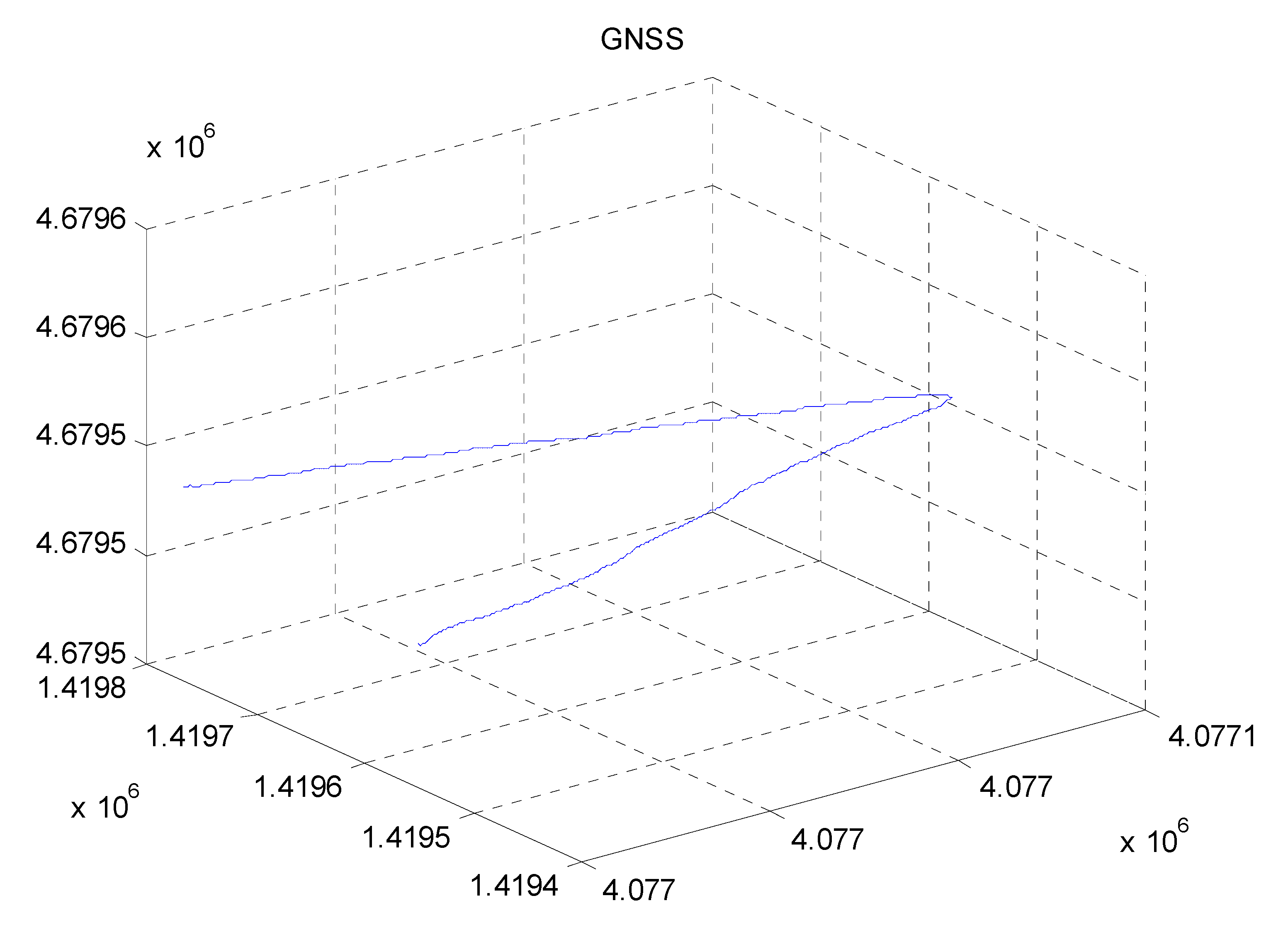
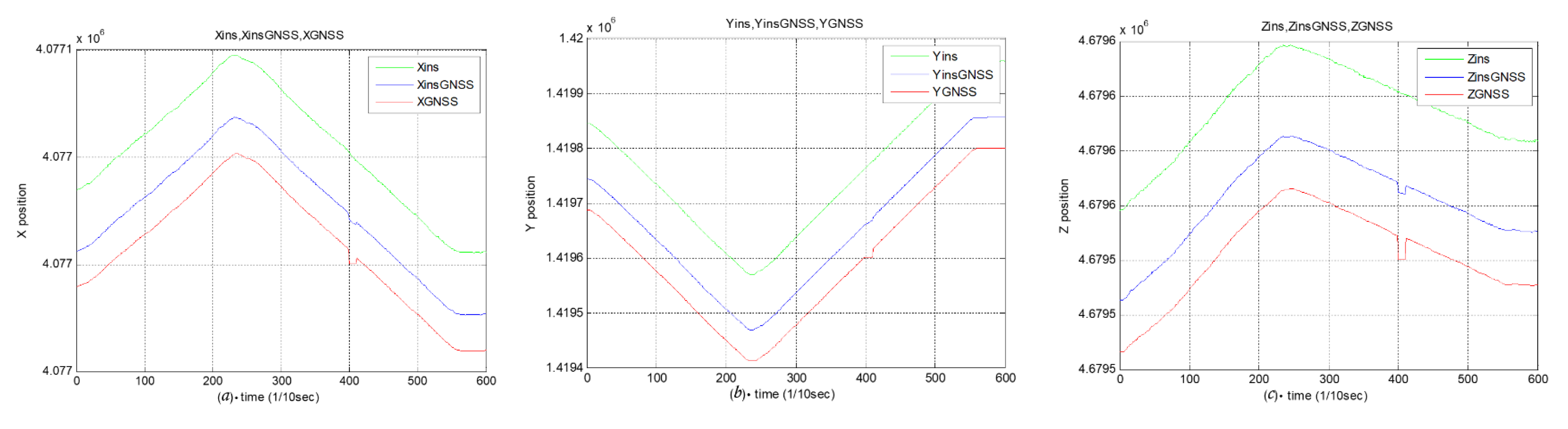
The INS and GNSS data used for the calculations were extracted from aircraft autopilot logs. The logs were produced when a video recording campaign was run at the Mátyásföld model airfield near Budapest, for Reference [26]. The data were recorded with a 3DR Iris+ [27] drone running the ArduCopter [28] firmware.

The INS information is available every 0.1 s, while the GNSS receiver information is available every one second. Nevertheless, the INS and GNSS must be time-synchronized to estimate the errors from the two frameworks in a specific time interval. Figure 3 shows the comparison of the drone trajectory coordinates in (X, Y, and Z) when using the (GNSS data without predictor) and (GNSS data with KNN predictor). From this figure, the drone’s trajectory in the three coordinates can be seen, represented by 60 points. At each point, GNSS provides the target position (X, Y, and Z). These points are 1 s apart, and hence the whole duration of the trajectory is 60 s.

The KNN predictor algorithm was used to enable GNSS receiver output to predict between samples instant when using the GNSS signal is lost for a few seconds. Hence, after adding the KNN predictor to the GNSS receiver’s output, it will have 600 points of (target position (X, Y, and Z)); these points are 0.1 s apart for the same whole 60 s duration of the trajectory.

The following scenarios are taken for the evaluation performance of the proposed GNSS/INS system (all of these scenarios are taken after adding the KNN predictor for the integration of GNSS/INS):

Scenario (І): 

This scenario compares the positions in three coordinates (X, Y, Z) for INS, GNSS, and the integration of GNSS/INS without blocking the GNSS data (see Figure 4).

Scenario (II): 

This scenario is like Scenario (I) but with a blocking time of 1 s in the GNSS receiver (see Figure 5).

Scenario (III): 

This scenario is like Scenario (II), but with a blocking time of 4 s in the GNSS receiver (see Figure 6).

Scenario (ІV): 

This scenario is like Scenario (III), but with a blocking time of 8 s in the GNSS receiver (see Figure 7).

From the above scenarios, one can conclude that using GNSS/INS with KNN predictor can decrease the deviation in the three coordinates (X, Y, and Z) when there is blocking in time (lost signal) for a few seconds in the GNSS receiver.

The standard deviation of INS, GNSS without predictor, and GNSS/INS with KNN predictor can be seen in

Table 1. The standard deviation of INS, GNSS without predictor, and GNSS/INS with KNN predictor, when the GNSS receiver with and without blocking in a few seconds.

GNSS	Standard Deviation
	${\mathit{\sigma }}_{\mathit{I}\mathit{N}\mathit{S}}$			${\mathit{\sigma }}_{\mathit{GNSS}}$ without KNN Predictor			${\mathit{\sigma }}_{\mathit{GNSS}/\mathit{INS}}$ with KNN Predictor
	X-Axis	Y-Axis	Z-Axis	X-Axis	Y-Axis	Z-Axis	X-Axis	Y-Axis	Z-Axis
No blocking	27.8269	117.5755	15.7477	27.6191	117.2243	15.8113	27.7402	117.4276	15.7710
1 s blocking	27.8269	117.5755	15.7477	27.5380	117.1091	15.6933	27.7465	117.4192	15.7247
4 s blocking	27.8269	117.5755	15.7477	27.4144	116.8594	15.3463	27.6745	117.1738	15.6184
8 s blocking	27.8269	117.5755	15.7477	26.6793	115.8801	15.0102	27.4085	116.6536	15.5051

, when the GNSS receiver with and without blocking in a few seconds. In References [13,14,15], different algorithm predictors to predict the output values of GPS were used, while, in this paper, a new algorithm was used to predict GNSS output values. Figure 5, Figure 6 and Figure 7 and Table 1 show the main results of this new method. Additionally, a brief evaluation of this research is shown in

Table 2. Brief evaluation of prediction methods.

Reference	Prediction for GPS or GNSS	Method of Predictor	Accuracy
[13]	GPS	NLMS	low
[14]	GPS	RBFNN and WNNs	better
[15]	GNSS	Carrier phase prediction	high
Our method	GNSS	KNN	high

.

4. Conclusions

The integration of GNSS and INS systems can make up for the weaknesses inherent in each and combine their individual advantages. Because the time synchronization between INS and GNSS must be achieved to estimate the errors from the two systems simultaneously, this paper adds a new technique of using a predictor on GNSS output before integrating with the INS. As a result, a prediction between the GNSS receiver’s sampling instants is required. The INS information is available every 0.1 s, while the GNSS receiver information is available every one second. Different predictors can be used for GNSS receivers, selecting the best one depending on its prediction results.

KNN predictor algorithm uses the database to search for data that is similar to the current data; hence, this algorithm is implemented at the output of the GNSS receiver to satisfy the synchronization process between INS and GNSS and predict the output of the GNSS receiver when its signal is lost (data blocking) for a few seconds. The ultra-tight integration of GNSS and INS was used in this study due to its advantages, such as anti-jamming immunity and increased dynamic ranges. The GNSS data were clutched in different scenarios, both with and without blocking for a few seconds. From the obtained results, it can be concluded that the error values in the three axes (X, Y, and Z) are increasing as the GNSS-data-blocking period is increased. In simple terms, whenever the GNSS data-blocking time is extended, the error values increase. Furthermore, the errors obtained when using GNSS/INS with predictor are less than INS alone, and GNSS without predictor for the same blocking periods in the GNSS data (see Figure 5, Figure 6 and Figure 7).

From Table 1, one can conclude that using GNSS/INS with the KNN predictor will make a smooth change in the standard deviation in all three axes, even when there is a blocking time in the GNSS receiver.

References

1. Meng, Y.; Gao, S.; Zhong, Y.; Hu, G.; Subic, A. Covariance matching based adaptive unscented Kalman filter for direct filtering in INS/GNSS integration. Acta Astronaut. 2016, 120, 171–181. [Google Scholar] [CrossRef]
2. Hu, G.; Wang, W.; Zhong, Y.; Gao, B.; Gu, C. A new direct filtering approach to INS/GNSS integration. Aerosp. Sci. Technol. 2018, 77, 755–764. [Google Scholar] [CrossRef]
3. Groves, P.D. Principles of GNSS, Inertial, and Multisensor Integrated Navigation Systems, 2nd ed.; Artech House: Boston, MA, USA, 2013; ISBN 978-1-60807-005-3. [Google Scholar]
4. Wang, W.; Liu, Z.Y.; Xie, R. rong Quadratic extended Kalman filter approach for GPS/INS integration. Aerosp. Sci. Technol. 2006, 10, 709–713. [Google Scholar] [CrossRef]
5. Hu, G.; Gao, S.; Zhong, Y.; Gao, B.; Subic, A. Modified federated Kalman filter for INS/GNSS/CNS integration. Proc. Inst. Mech. Eng. Part G J. Aerosp. Eng. 2016, 230, 30–44. [Google Scholar] [CrossRef]
6. Quan, W.; Li, J.; Gong, X.; Fang, J. INS/CNS/GNSS Integrated Navigation Technology; Springer: Berlin/Heidelberg, Germany, 2015; ISBN 978-3-662-45158-8. [Google Scholar] [CrossRef]
7. Noureldin, A.; Karamat, T.B.; Eberts, M.D.; El-Shafie, A. Performance enhancement of MEMS-based INS/GPS integration for low-cost navigation applications. IEEE Trans. Veh. Technol. 2009, 58, 1077–1096. [Google Scholar] [CrossRef]
8. Nemra, A.; Aouf, N. Robust INS/GPS sensor fusion for UAV localization using SDRE nonlinear filtering. IEEE Sens. J. 2010, 10, 789–798. [Google Scholar] [CrossRef] [Green Version]
9. Fang, J.; Gong, X. Predictive iterated kalman filter for INS/GPS integration and its application to SAR motion compensation. IEEE Trans. Instrum. Meas. 2010, 59, 909–915. [Google Scholar] [CrossRef]
10. Abbott, A.S.; Lillo, W.E. Global Positioning Systems and Inertial Measuring Unit Ultratight Coupling Method. U.S. Patent 6516021B1, 4 February 2003. [Google Scholar]
11. Falco, G.; Pini, M.; Marucco, G. Loose and tight GNSS/INS integrations: Comparison of performance assessed in real Urban scenarios. Sensors 2017, 17, 255. [Google Scholar] [CrossRef] [PubMed]
12. Bernal, D.; Closas, P.; Fernández-Rubio, J.A. Particle filtering algorithm for ultra-tight GNSS/INS integration. In Proceedings of the 21st International Technical Meeting of the Satellite Division of the Institute of Navigation, ION GNSS 2008, Savannah, GA, USA, 16–19 September 2008; Volume 1, pp. 239–246. [Google Scholar]
13. Abdul-kaliq Abdul-aziez, S.; Yass, M.; Jassim Mohammed, H. NLMS Adaptive Filter Algorithm Method for GPS Data Prediction; IAJS: Baghdad, Iraq, 2016; Volume 6. [Google Scholar]
14. Mahel Mohammed, F.; Aziez, S.A.; Naji Abdul-Rihda, H. Comparison between Wavelet and Radial Basis Function Neural Networks for GPS Prediction; IAJS: Baghdad, Iraq, 2015. [Google Scholar]
15. Li, Z.; Zhang, T.; Qi, F.; Tang, H.; Niu, X. Carrier phase prediction method for GNSS precise positioning in challenging environment. Adv. Space Res. 2019, 63, 2164–2174. [Google Scholar] [CrossRef]
16. Kaghyan, S.; Sarukhanyan, H. Activity recognition using K-nearest neighbor algorithm on smartphone with Tri-axial accelerometer. Int. J. Inform. Models Anal. 2012, 1, 146–156. [Google Scholar]
17. Sinta, D.; Wijayanto, H.; Sartono, B. Ensemble K-Nearest neighbors method to predict rice price in Indonesia. Appl. Math. Sci. 2014, 8, 7993–8005. [Google Scholar] [CrossRef] [Green Version]
18. Imandoust, S.B.; Bolandraftar, M. Application of K-Nearest Neighbor (KNN) Approach for Predicting Economic Events: Theoretical Background. Int. J. Eng. Res. Appl. 2013, 3, 605–610. [Google Scholar]
19. Grewal, M.S.; Andrews, A.P. Kalman Filtering: Theory and Practice with MATLAB, 4th ed.; Wiley-IEEE Press: Hoboken, NJ, USA, 2014; ISBN 1118851218. [Google Scholar]
20. Ribeiro, M.I. Kalman and Extended Kalman Filters: Concept, Derivation and Properties. Inst. Syst. Robot. Lisb. Port. 2004, 42, 46. [Google Scholar]
21. Raja, M.; Sidhu, H.S.; Adhiyaman, N.; Teja, A.K. Integration of GPS/INS Navigation System with Application of Fuzzy Corrections. In Proceedings of the Conference on Advances in Communication and Control Systems 2013 (CAC2S 2013), Uttarakhand, India, 6–8 April 2013; Volume 2013, pp. 450–454. [Google Scholar]
22. Ismaeel, S.A. Design of Kalman Filter of Augmenting GPS to INS Systems. Master’s Thesis, Computer Engineering Department College of Engineering Al-Nahrain University, Baghdad, Iraq, 2003; pp. 59–66. [Google Scholar]
23. Babu, R.; Wang, J. Ultra-tight GPS/INS/PL integration: A system concept and performance analysis. GPS Solut. 2009, 13, 75–82. [Google Scholar] [CrossRef]
24. Bhatti, U.I. Improved Integrity Algorithms for Integrated GPS/INS Systems in the Presence of Slowly Growing Errors Declaration of Contribution. Ph.D. Thesis, University of London, London, UK, 2007. [Google Scholar]
25. Yan, Z.; Chen, X.; Tang, X. A novel linear model based on code approximation for GNSS/INS ultra-tight integration system. Sensor 2020, 20, 3192. [Google Scholar] [CrossRef] [PubMed]
26. Hiba, A.; Szabo, A.; Zsedrovits, T.; Bauer, P.; Zarandy, A. Navigation data extraction from monocular camera images during final approach. In Proceedings of the 2018 International Conference on Unmanned Aircraft Systems (ICUAS), Dallas, TX, USA, 12–15 June 2018; pp. 340–345. [Google Scholar] [CrossRef]
27. 3DR Iris+. Available online: https://www.adafruit.com/product/2199 (accessed on 27 May 2021).
28. Copter Home—Copter documentation. Available online: https://ardupilot.org/copter/ (accessed on 27 May 2021).
Figure 1. The 3D trajectory of the moving drone.
Electronics 10 01513 g001
Figure 2. Kalman filter for ultra-tightly coupled GNSS/INS Integration.
Electronics 10 01513 g002
Figure 3. Comparing the drone trajectory coordinates in (X, Y, and Z) when using the GNSS data without predictor and GNSS data with KNN predictor; a-1 shows the drone trajectory in X-axis without using KNN predictor; a-2 shows the drone trajectory in X-axis by using the KNN predictor; b-1 shows the drone trajectory in Y-axis without using KNN predictor; b-2 shows the drone trajectory in Y-axis by using the KNN predictor; c-1 shows the drone trajectory in Z-axis without using KNN predictor; c-2 shows the drone trajectory in Z-axis by using the KNN predictor.
Electronics 10 01513 g003aElectronics 10 01513 g003b
Figure 4. Comparing between the positions in three coordinates (X, Y, and Z), for INS, GNSS, and integration of GNSS/INS without blocking in the GNSS data; a shows the INS, GNSS, and integration of INS/GNSS routes in X-axis without GNSS blocking; b shows the INS, GNSS, and integration of INS/GNSS routes in Y-axis without GNSS blocking; c shows the INS, GNSS, and integration of INS/GNSS routes in Z-axis without GNSS blocking.
Electronics 10 01513 g004aElectronics 10 01513 g004b
Figure 5. Comparing between the positions in three coordinates (X, Y, and Z) for INS, GNSS, and integration of GNSS/INS when blockings of (1 s) are accord in the GNSS data; a shows the INS, GNSS, and integration of INS/GNSS routes in X-axis with one second of GNSS blocking; b shows the INS, GNSS, and integration of INS/GNSS routes in Y-axis with one second of GNSS blocking; c shows the INS, GNSS, and integration of INS/GNSS routes in Z-axis with one second of GNSS blocking.
Electronics 10 01513 g005
Figure 6. Comparing between the positions in three coordinates (X, Y, and Z) for INS, GNSS, and integration of GNSS/INS through blockings of (4 s) are accord in the GNSS data; a shows the INS, GNSS, and integration of INS/GNSS routes in X-axis with 4 s of GNSS data blocking; b shows the INS, GNSS, and integration of INS/GNSS routes in Y-axis with 4 s of GNSS data blocking; c shows the INS, GNSS, and integration of INS/GNSS routes in Z-axis with 4 s of GNSS data blocking.
Electronics 10 01513 g006
Figure 7. Comparing between the positions in three coordinates (X, Y, and Z) for INS, GNSS, and integration of GNSS/INS when blockings of (8 s) are accord in the GNSS data; a shows the INS, GNSS, and integration of INS/GNSS routes in X-axis with 8 s of GNSS data blocking; b shows the INS, GNSS, and integration of INS/GNSS routes in Y-axis with 8 s of GNSS data blocking; c shows the INS, GNSS, and integration of INS/GNSS routes in Z-axis with 8 s of GNSS data blocking.
Electronics 10 01513 g007