Dirt Loss Estimator for Photovoltaic Modules Using Model Predictive Control

Abstract

The central problem tackled in this article is the susceptibility of the solar modules to dirt that culminates in losses in energy generation or even physical damage. In this context, a solution is presented to enable the estimates of dirt losses in photovoltaic generation units. The proposed solution is based on the mathematical modeling of the solar cells and predictive modeling concepts. A device was designed and developed to acquire data from the photovoltaic unit; process them based on a predictive model, and send loss estimates in the generation unit to a web server to help in decision-making support. The results demonstrated the real applicability of the system to estimate losses due to dirt or electrical mismatches in photovoltaic plants.

1. Introduction

Photovoltaic conversion is the direct energy transformation from solar radiation into electrical energy through the photovoltaic effect. The electrical energy obtained can then be injected into the electrical grid by some power electronics converter, giving rise to the mini and micro photovoltaic generation systems. Since the enactment of the resolution of the National Electric Energy Agency (ANEEL), number 482/2012, which regulated the mini and microgeneration distributed systems in Brazil, the usage of photovoltaic solar energy has expanded, achieving thousands of new installations each year [1,2].

It is well-known that photovoltaic solar energy presents financial and ecological benefits associated with the strident reduction in costs for implementing generation systems. The photovoltaic technology has emerged as a trend in the electricity market, once it is a viable solution for the electricity supply by companies and customer. This fact is corroborated by international agencies, which predict that photovoltaic energy increases from 2% of the world energy matrix in 2018 to 25% in 2050 [3].

Despite the many benefits as a source for distributed generation, photovoltaic (PV) modules are sensitive to the accumulation of dust and residues on their surface, causing efficiency reduction common to all generation units. Dirt losses can vary from 2% to 25%, maintaining an average of 5%. The deposit of dirt on the modules’ surface has been a research subject in several aspects: qualitative, quantitative, and economic [4,5,6,7,8,9,10,11].

One study focuses on determining the appropriate time interval for cleaning modules, proposing a preventive solution; that is, clean the modules at pre-established intervals [8]. It turns out that the seasons of the year imply different climatic conditions, as rains, winds, and air humidity, which may require monthly or biannual cleaning, especially if it is considered the location and conditions of the generation unit installation. For instance, a module installed on a building tends to accumulate less dirt than another installed on the ground; in the same sense, summer rainfalls tend to keep the modules cleaner in this period. The neighborhood also impacts the efficiency of the generation units. The presence of a construction site close to the region of the generation unit may generate a soiling accumulation quickly. In this scenario, a suitable cleaning interval is not feasible and tends to incur unnecessary cleaning or the module’s efficiency losses due to late cleaning.

Another aspect, observed in [9], is the determination of dirt losses related to the country regions, as well as the technology of the photovoltaic module. According to the authors, modules of cadmium telluride (CdTe) and polycrystalline silicon (p-Si) have different levels of losses for the same level of dirt. In this analysis, the amorphous silicon and CdTe modules lost performance more suddenly due to the deposition of dirt than those of crystalline silicon technology due to the difference between their spectral response ranges.

The work presented in [8,9] suggests a quantitative approach to dirt losses through a relationship between the output power of the generation unit and the solar irradiance simultaneously interval. The proposal estimates of how much energy should be generated are obtained for a given availability of solar radiation. However, they do not update the parameters of the cell model so leading to estimation errors.

The authors in [10] suggest a model based on the relationship between the transmittance at a certain angle of incidence, which varies according to the dirt and the transmittance in conditions without dirt. The proposed model is an extension of the model adopted by the American Society of Heating, Refrigeration and Air Conditioning but requires using empirical adjustment parameters that assume vague dirt conditions at levels, such as low, medium, and high.

The model predictive control (MPC) has shown real feasibility and applicability in several prediction systems [12,13]. To the best of our knowledge, the usage of MPC to estimate losses in photovoltaic systems is not found in the literature, considering the incident irradiance, the irradiance absorbed, and the online estimation of the series resistance of the PV module, with analysis through time. Considering the need for increasing efficiency in photovoltaic energy production, this work presents the estimation of losses by a new model, based on MPC, which is robust and flexible to be applied in systems with nonlinearities as observed in photovoltaic systems.

2. Materials and Methods

2.1. Losses Estimation

The generated energy depends directly on the intensity of the radiation, the temperature, anomalies, such as shading and dirt. Dirt reduces the efficiency of the generation system and compromises the module’s lifetime due to abnormal cell heating. Therefore, the estimation of dirt is an aid tool in the decision-making process to perform module cleanup.

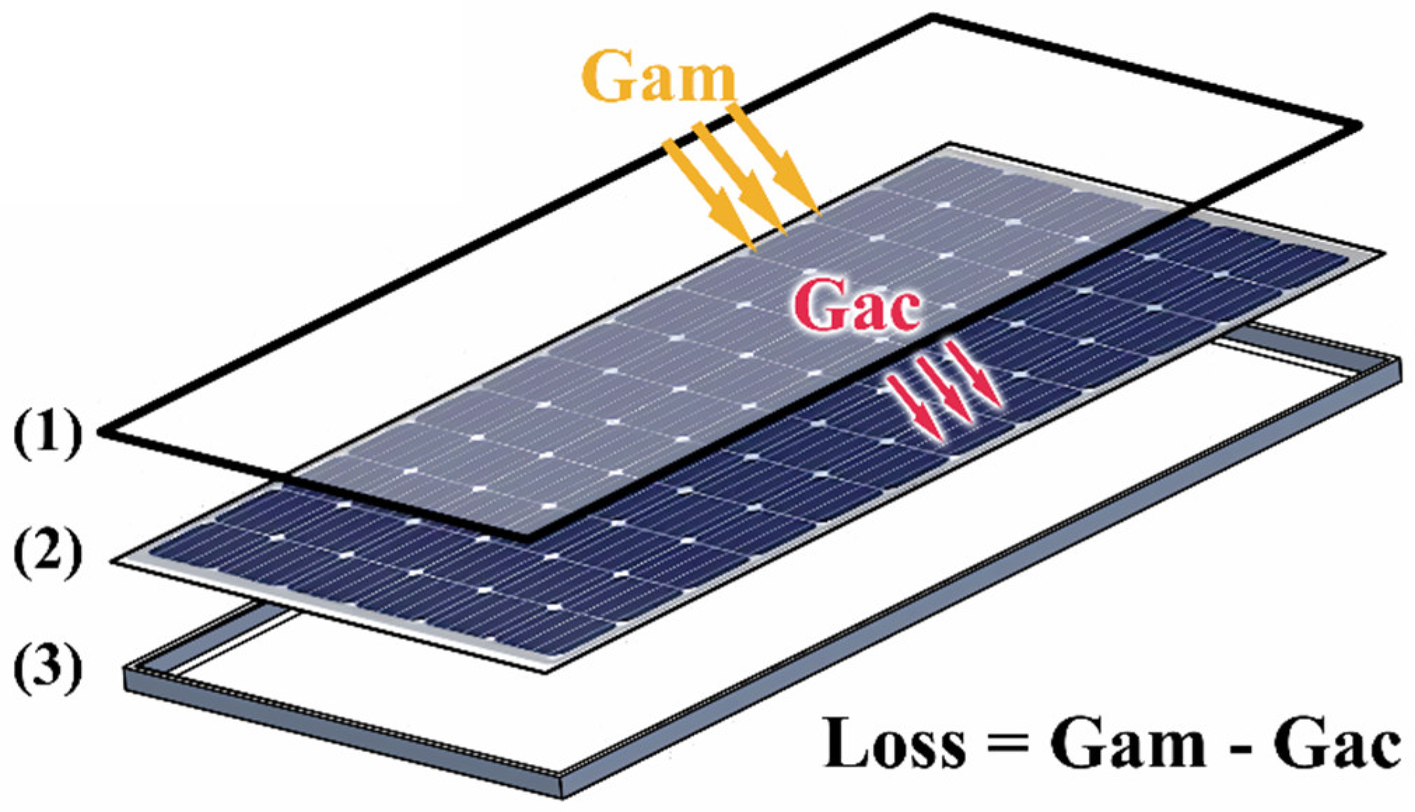
The photovoltaic cells receive solar irradiance (G_am) that is converted into electrical energy, producing a current (I_cel) for a given voltage (V_Cel). By applying I_Cel and V_Cel to an estimation system based on MPC and the mathematical model of the PV cell, one may obtain the irradiance that originated this current and voltage, which will be called calculated irradiance (G_ac). The difference between G_am and G_ac represents the unused irradiance on the surface of the module, as shown in Figure 1.

Once some photovoltaic cell parameters are difficult to be measured dynamically [14,15,16], this work estimates energy losses by adopting the MPC modeling.

Regarding the module’s physical structure, there are other materials between the front glass and the cells, such as an EVA layer. Since this work deals with the estimation of losses based on the difference between measured and calculated irradiance, the determination of dirt does not depend on the particles or the physical composition of the module.

2.2. Mathematical PV Modeling

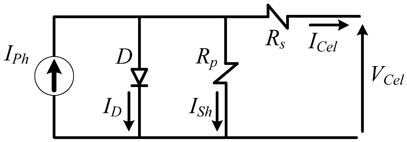
Figure 2 shows the approximate fundamental cell model with four parameters. The series resistor R_s and the parallel resistor R_p represent the non-idealities [14].

The output current is presented in (1):

$$I_{Cel}=I_{Ph}-I_D-I_{Sh},$$

(1)

where $I_{Ph}$ is the photocurrent, $I_D$ the diode reverse saturation current and $I_{Sh}$ the current in the parallel resistance. $I_{Ph}$, which depends on solar irradiance and temperature, is featured in (2); $I_D$ and $I_{Sh}$ are presented in (3) and (4), respectively:

$$I_{Ph}=\frac{G_a{I}_{sc}}{G{a}_{Ref}}+K_0\left(T_c-T_{ref}\right),$$

(2)

$$I_D=\frac{I_{sc}}{e^{\frac{q{V}_{oc}}{nk{T}_{Ref}}}-1} {\left(\frac{T_c}{T_{Ref}}\right)}^{\frac{3}{n}}{e}^{\frac{-q{E}_g}{nk} \left(\frac{1}{T_{Ref}}-\frac{1}{T_C}\right)} \left[e^{\frac{q}{nk{T}_c}\left(V_{Cel}+R_s{I}_{Cel}\right)}-1\right],$$

(3)

$$I_{Sh}=\frac{\left(V_{Cel}+R_S{I}_{Cel}\right)}{R_p}.$$

(4)

Substituting (2)–(4) in (1), we find the output current of the solar cell according to (5).

Table 1. Main variables of (5).

Element	Value
Elementary charge	q = 1.6 × 10−19 C
Boltzmann constant	k = 1.38 × 10−23 J/K
Ideality factor	n = 1.2
Prohibited band energy	Eg = 1.12 eV
Reference temperature	Tref = 298 K
Temperature	Tc (K)
Irradiance	Ga (W/m2)
Irradiance reference	Garef = 1000 W/m2
Current variation coefficient	K0 (A/K)
Short-circuit current	ISC (A)
Open-circuit voltage	Voc (V)
Diode saturation current at Tref	ISRef (A)

summarizes the main variables of (5):

$$I_{Cel}\frac{G_a{I}_{sc}}{G{a}_{Ref}}+{\mathrm{K}}_0\left(T_c-T_{ref}\right)-I_{SRef}{\left(\frac{T_c}{T_{Ref}}\right)}^{\frac{3}{n}}{e}^{\frac{-q{E}_g}{nk} \left(\frac{1}{T_{Ref}}-\frac{1}{T_C}\right)} \left[e^{\frac{q}{nk{T}_c}\left(V_{Cel}+R_s{I}_{Cel}\right)}-1\right]-\frac{\left(V_{Cel}+R_s{I}_{Cel}\right)}{R_p},$$

(5)

where $I_{SRef}$ is the saturation diode current at $T_{Ref}$.

$$I_{SRef}=\frac{I_{sc}}{e^{\frac{q{V}_{oc}}{nk{T}_{Ref}}}-1}.$$

(6)

2.3. Irradiance Estimation Modeling

The estimation system is based on the photovoltaic cell model presented in (5). The module receives direct irradiation and delivers electrical energy. Therefore, reorganizing (5) using the irradiance (Gac), the proposed model is obtained. The proposed model operates differently from the conventional model, so that outputs the irradiance in terms of the output voltage and current, as well as the temperature and internal resistances of the photovoltaic cell, as described in (7):

$$G_{ac}=\frac{G{a}_{ref}}{I_{sc}}\{I_{Cel}-{\mathrm{K}}_0\left(T_c-T_{ref}\right)+I_{SRef}{\left(\frac{T_c}{T_{Ref}}\right)}^{\frac{3}{n}}{e}^{\frac{-q{E}_g}{nk} \left(\frac{1}{T_{Ref}}-\frac{1}{T_C}\right)} \left[e^{\frac{q}{nk{T}_c}\left(V_{Cel}+R_s{I}_{Cel}\right)}-1\right]+\frac{\left(V_{Cel}+R_s{I}_{Cel}\right)}{R_p}\}$$

(7)

Using the solar irradiance calculated according to (7), as well as the irradiance measured using a radiometer and, considering a module under normal operating conditions, one may calculate the losses percentage in the photovoltaic module (8):

$$Losses (\%)=\frac{G_{am}-G_{ac}}{G_{am}}100(\%).$$

(8)

2.4. Determination of Series and Parallel Resistances

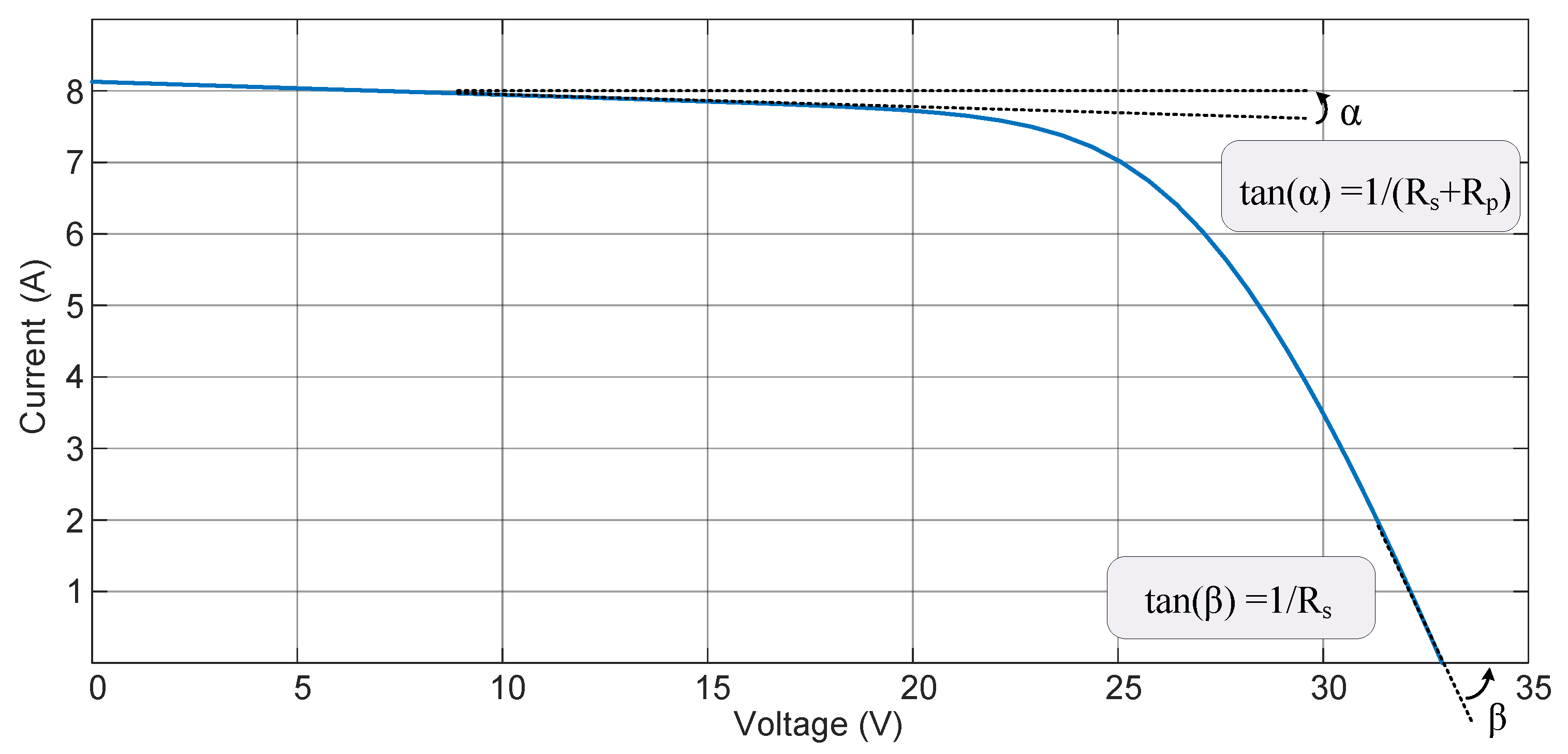
The series and parallel resistances affect the cell’s normal functioning in a different manner, but both flatten the characteristic I–V curve. In Figure 3, as the R_p value is reduced, the I–V curve becomes a straight line with a slope of 1/(R_p + R_s) in the region known as the current source. When the R_s value is increased, the curve is a straight line with an inclination of 1/R_s in the voltage source region. Therefore, for high values of R_s and low values of R_p, the I–V curve will have a shape of a rectangle. One way to calculate the instantaneous value of the series resistance is obtained by differentiating (1) in relation to the voltage, when V_Cel = V_OC, and isolating R_s, obtaining (9).

$$R_S=-\frac{d{V}_{Cel}}{d{I}_{Voc}}-\frac{1}{\frac{\frac{G_a{I}_{sc}}{G{a}_{Ref}}q}{nk{T}_{ref}} e^{\frac{q{V}_{oc}}{nk{T}_{ref}}}}.$$

(9)

I_Voc is the output current considered when V_Cel = V_OC, that is, at the limit of the open-circuit voltage. In the first part of Equation (9), the β slope of the I–V curve appears, as shown in Figure 3. The second part inserts the effects of solar irradiance and the output voltage. Solving (9) is non-trivial. As a solution for the dynamic R_s value, this work proposes its estimation through the MPC.

The parallel resistance R_p comes from constructive characteristics of the cell due to the insertion of impurities, which culminate in providing an internal path of low impedance to the current, which appears parallel to the current source I_Ph in Figure 2. The parallel resistance depends linearly on the temperature, and it is inversely proportional to the irradiance. R_p is calculated in (10). R_Pref was obtained from a curve plotter in the STC conditions, and the methodology was pointed out in [14]. R_Pref was set as a fixed value, as it has little impact on the estimation [2]. The STC condition was validated with an irradiance sensor:

$$R_P=\frac{G{a}_{Ref}}{Ga}R{p}_{ref}.$$

(10)

2.5. Predictive Modeling

The MPC algorithm predicts the values of a signal or variable, identifies patterns or Please ensure your intended meaning was retained [2,13]. Predictive control relies on mathematical representation in the state space of the plant to design the configuration of the controller. In the configuration, the future outputs of a given prediction horizon are estimated at each timestamp (t).

State and output prediction is based on two parameters to design the Predictive controller: control horizon (N_c) and prediction horizon (N_p). The control horizon is the number of parameters needed to reach the future control path. Given the state vector x, the future state vector can be predicted with N_p samples. The prediction horizon defines the size of the cost function optimization window. Through the prediction horizon, it is determined how many future time intervals are intended to predict the outputs to estimate the necessary performance of the manipulated variable.

Following the guidelines presented in [12], the predictive model is based on the modeling of plants through the state space according to (11):

$$\begin{array}{c}{\mathrm{x}}_{\mathrm{m}}\left(\mathrm{t}\right)=A_m{\mathrm{x}}_{\mathrm{m}}\left(\mathrm{t}\right)+B_m\Delta \mathrm{u}\left(\mathrm{t}\right)\\ \mathrm{y}\left(\mathrm{t}\right)=C_m{\mathrm{x}}_{\mathrm{m}}\left(\mathrm{t}\right)\end{array}$$

(11)

Equation (12) represents the discrete form.

$$\begin{array}{c}\mathrm{x}\left(\mathrm{k}+1\right)=A\mathrm{x}\left(\mathrm{k}\right)+B\Delta \mathrm{u}\left(\mathrm{k}\right)\\ \mathrm{y}\left(\mathrm{k}\right)=C\mathrm{x}\left(\mathrm{k}\right)\end{array}$$

(12)

The plant state–space matrices are used to find the augmented matrices [13], which are the basis of the predictive control design. The augmented matrices A, B and C are generated according to (13)–(15), respectively:

$$A=\left[\begin{array}{cc}{A}_m& o_m^T\\ C_m{A}_m& 1\end{array}\right],$$

(13)

$$B=\left[\begin{array}{c}{B}_m\\ C_m{B}_m\end{array}\right]$$

(14)

$$C=\left[\begin{array}{cc}{o}_m& 1\end{array}\right],$$

(15)

where $o_m=\left[\begin{array}{cc}0& 0\end{array}\right]$.

Based on the augmented matrices, matrices F and ϕ are defined, in which the dimensions directly depend on the choice of Nc and Np. Matrices F and ϕ are presented in (16) and (17), respectively:

$$F=\left[\begin{array}{c}CA\\ C{A}^2\\ C{A}^3\\ ⋮\\ C{A}^{N_p}\end{array}\right]$$

(16)

$$\varnothing =\left[\begin{array}{ccccc}CA& 0& 0& \cdots & 0\\ CAB& CB& 0& \cdots & 0\\ C{A}^2& CAB& CB& \cdots & 0\\ ⋮& ⋮& ⋮& ⋮& ⋮\\ C{A}^{N_p-1}B& C{A}^{N_p-2}B& C{A}^{N_p-3}B& \cdots & C{A}^{N_p-N_c}B\end{array}\right]$$

(17)

The optimal solution that defines the action of the MPC controller is presented in (18) [13]:

$$\Delta U={\left({\varnothing }^T\varnothing +\overline{R}\right)}^{-1}{\varnothing }^T({\overline{R}}_s\mathrm{r}\left({\mathrm{k}}_{\mathrm{i}}\right)-F\mathrm{x}\left({\mathrm{k}}_{\mathrm{i}}\right)),$$

(18)

where ${\left({\varnothing }^T\varnothing +\overline{R}\right)}^{-1}$ is defined as the Hessian Matrix and ${\overline{R}}_s\mathrm{r}\left({\mathrm{k}}_{\mathrm{i}}\right)$ is related to the operation point of the system.

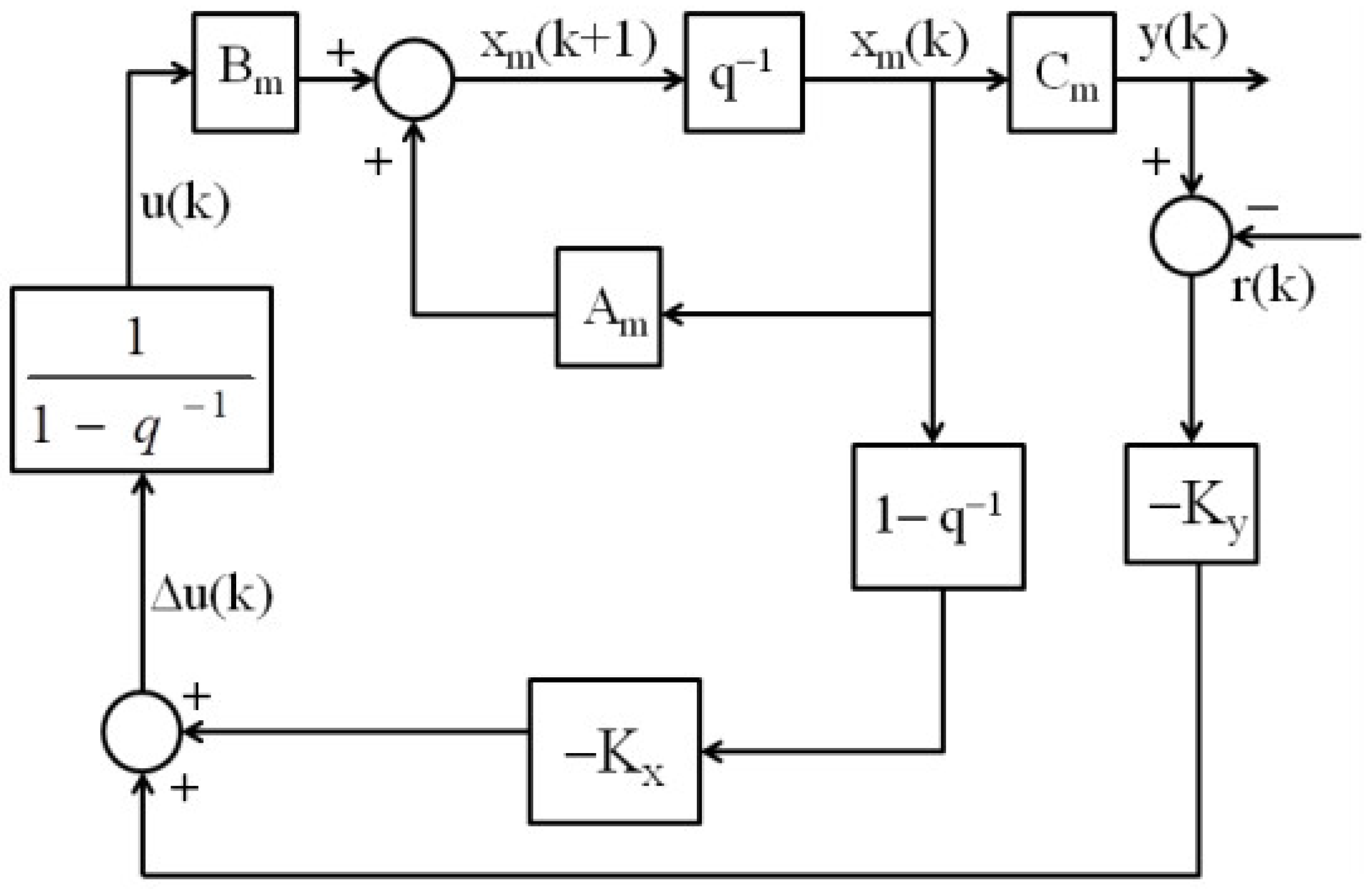
The gain of the MPC controller is presented in (19), considering N_c = 4 and, (20) presents the MPC controller output, with $K_{MPC}=\left[\begin{array}{cc}{\mathrm{K}}_{\mathrm{x}}& {\mathrm{K}}_{\mathrm{y}}\end{array}\right]$. Figure 4 depicts the final configuration of the control as a block diagram:

$$K_{MPC}=\stackrel{\mathrm{Nc}}{\overbrace{\left[1000\right]}}{\left({\varnothing }^T\varnothing +\overline{R}\right)}^{-1}\left({\varnothing }^{T}F\right),$$

(19)

$$Y\left(\mathrm{k}\right)=F\mathrm{x}\left({\mathrm{k}}_{\mathrm{i}}\right)+\varnothing \Delta U$$

(20)

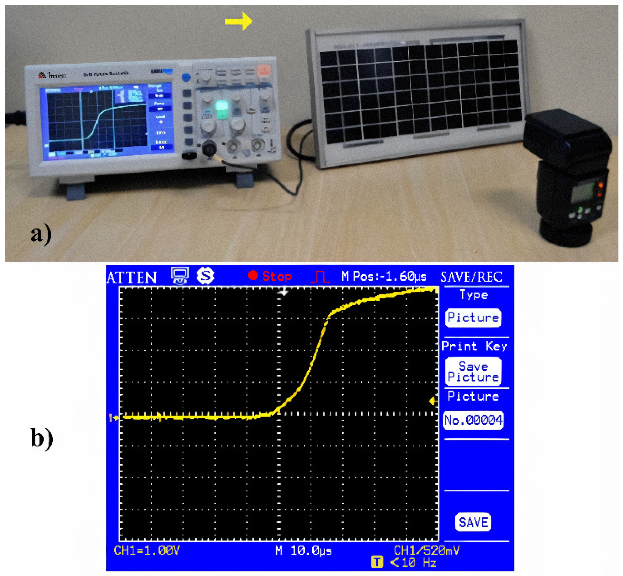
A reduced reference PV model (excited by a flashlight) has been used to obtain the state space representation of the PV system. The reference module has the specifications for the MPP point, 8.8 A and 5.1 V. The irradiance obtained by the light beam was of the order of 400 W/m², a current of approximately 3.5 A was drained. Figure 5 presents the PV system (5a) and the step response obtained with an oscilloscope.

As a first-order system, the transfer function is presented in its standard form by (21). The term K represents the plant gain and τ the system time constant, according to (22) and (23), where ∆E is the variation of the input and ∆S is the variation of the output.

Observing the response to the step, Figure 5, it is possible to verify Te = 20 μs; ∆E = 1 and ∆S = 3. Thus, the transfer function is given by (24):

$$G\left(s\right)=\frac{K}{\tau s+1}$$

(21)

$$K=\frac{\Delta S}{\Delta E}$$

(22)

$$\tau =\frac{Te}{4}$$

(23)

$$G\left(s\right)=\frac{3}{5\times {10}^{-6}s+1}$$

(24)

Adopting Ts = 0.4 µs, (25) and (26) were obtained, which represent the discrete state–space model of the photovoltaic module:

$$x\left(k+1\right)=Ax\left(k\right)+Bu\left(k\right)$$

(25)

$$y\left(k\right)=Cx\left(k\right)$$

(26)

Based on the prediction of the state variable, the predicted outputs behave according to (27):

$$\begin{array}{c}y\left(k_i+N_p|k_i\right)=C{A}^{N_p}x\left(k_i\right)+C{A}^{N_{p-1}}B\Delta u\left(k_i\right)+C{A}^{N_{p-2}}B\Delta u\left(k_i+1\right)+\cdots +\\ C{A}^{N_p-N_c}B\Delta u\left(k_i+N_c-1\right),\end{array}$$

(27)

where A = 0.9048, B = 3.807 × 10⁻⁷ and C = 7.5 × 10⁵.

The predicted outputs are used to estimate the best range for Rs. N_p = 5 and N_c = 4 were adopted, and these values were defined from the best performance of the response from computer simulations.

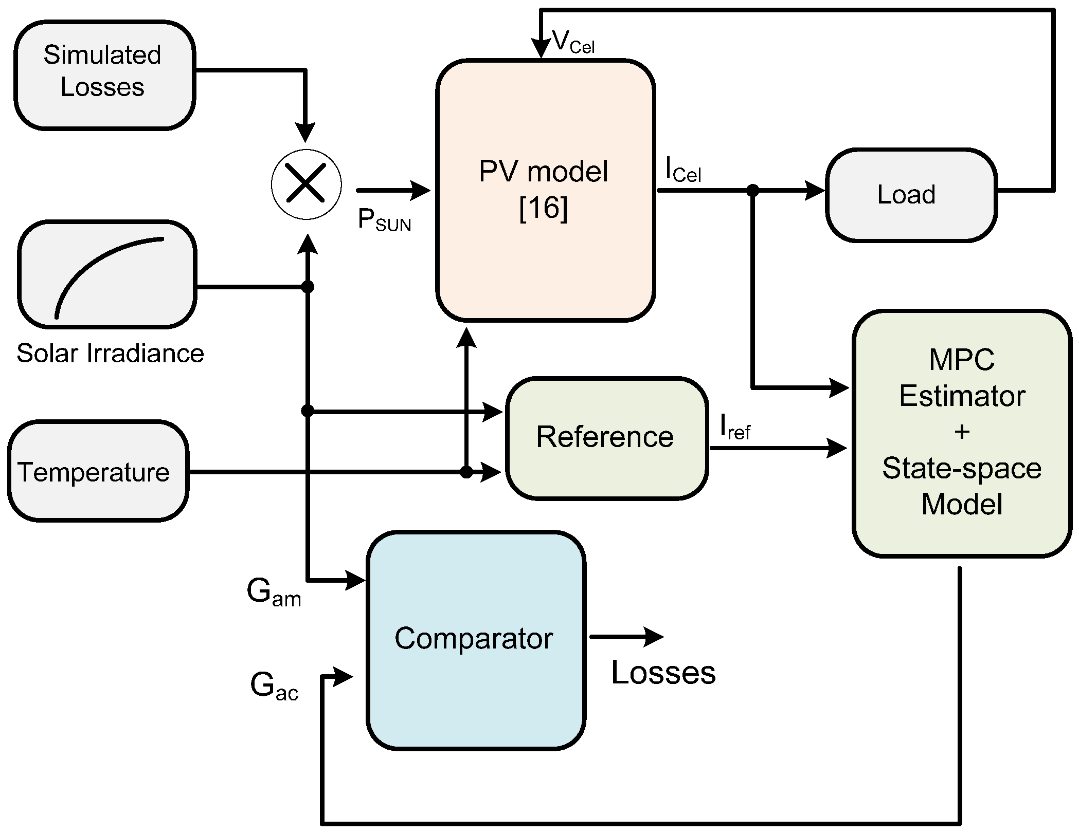
Figure 6 shows a block diagram of the MPC estimator with the insertion of the predictive control model. The Reference block provides the reference for the MPC module, supplying the module current under ideal conditions of temperature and irradiance. The MPC controller, together with the state–space model, estimates the energy losses of the photovoltaic module.

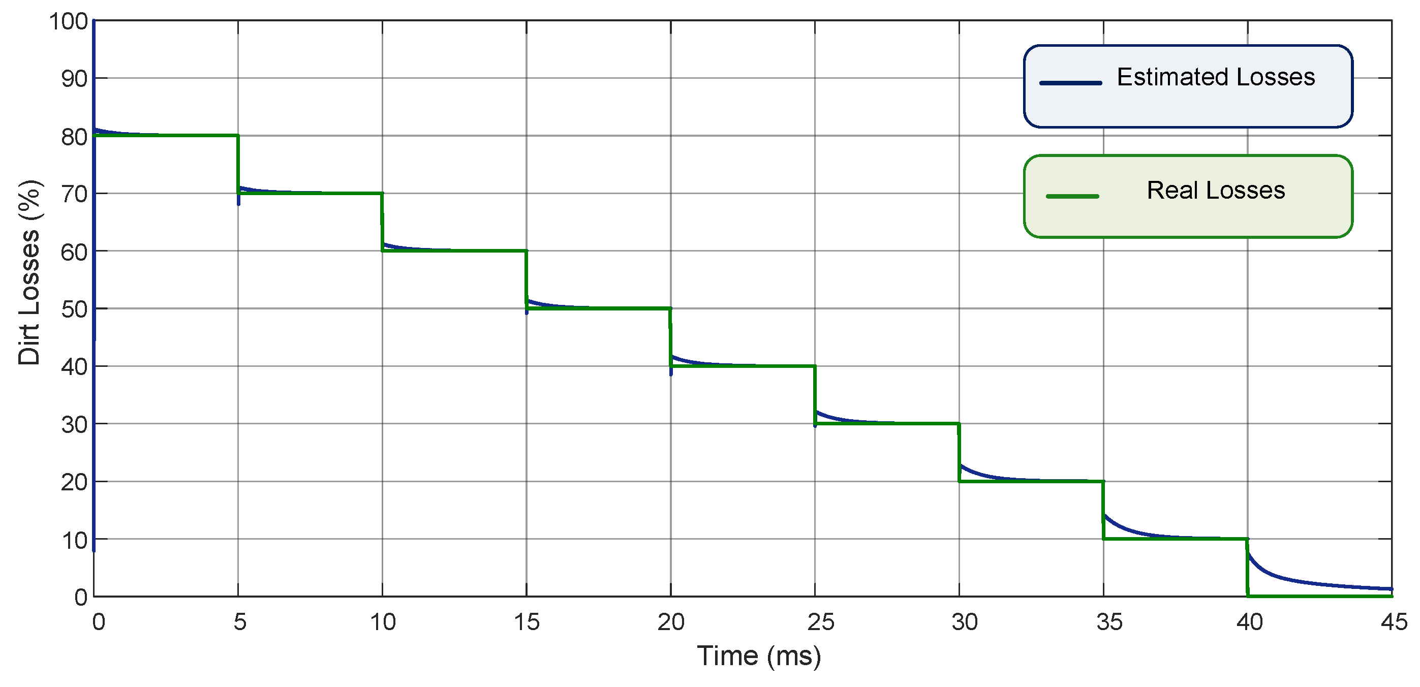
Figure 7 presents the results of a comparison between real dirt losses, and a simulation performed using the MPC-based estimator (losses ranging from 80% down to 0%). The proposed model correctly estimates the R_s values to predict the actual PV losses.

Table 2. Influence of irradiation on the R_s parameter.

Irradiance (W/m2)	Rs (mΩ)
200–300	120.50
300–400	92.30
400–500	60.85
500–600	30.80
600–700	18.10
700–800	12.80
800–900	9.30
900–1000	6.50
>1000	4.00

presents the R_s estimated values.

The Rs values represent the first-order portion in the differential equation presented in (9), considering the operation at the maximum power point (MPP) for various irradiance levels.

3. Results and Discussions

The energy losses MPC estimator is based on the mathematical model of the solar cell for calculating G_ac, as well as on the predictive model for estimating an approximation for Rs. In the block diagram presented in Figure 6, the difference between G_ac and G_am shows how much energy was not absorbed on the front surface of the PV module.

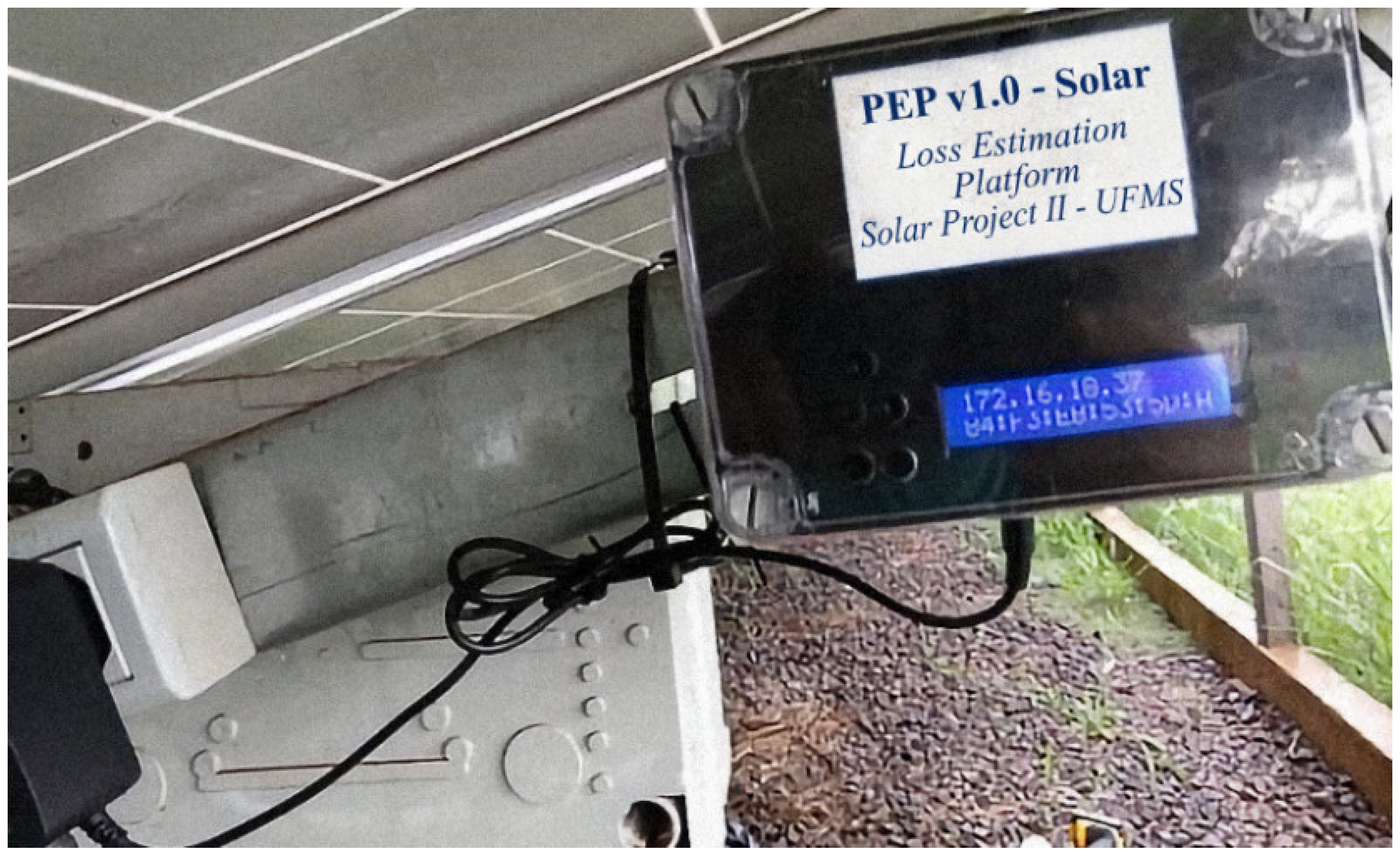
We have designed and prototyped an embedded device that implements the MPC estimator. The device was fitted to the available space in conventional string boxes, and it was installed next to the sectioning elements and DC protection of the generation unit. Figure 8 shows the prototype at the Federal University of Mato Grosso do–Sul photovoltaic solar plant (UFV-UFMS), being connected directly at the output of the arrangement. The device was built to withstand a maximum voltage of up to 900 V and a current of up to 30 A. The prototype has a Microchip DSPic 30F4013 processor as a logical unit and possesses Wi-Fi, RS-232, a USB communication system, a PT-1000 temperature sensor, and a radiometer reading of up to 1300 W/m². The voltage acquired by the device is divided by the number of series modules to properly feed the estimation model.

The UFV-UFMS is comprised of 38 PV modules (model CS6K-275P), each one of 275 Wp, organized into two strings of 19 modules, each connected in series, being both connected in parallel to a string-box, forming an array with 10.45 kWp maximum power. Each module has a short-circuit current of 9.45 A, open-circuit voltage of 38 V, the current and voltage at the MPP point are 8.88 A and 31 V, respectively. Under STC conditions (25 °C and 1000 W/m²), the array has an open-circuit voltage (V_oc) of 722 V and a short-circuit current of 18.9 A. The measured parameters of the photovoltaic arrangement are adapted (dividing the current by the number of strings and dividing the voltage by the number of modules and cells of each module) to match the model input data. The energy losses estimate, on average, the soiling on the whole set of PV modules. The PV power plant has an 8.2 kW Fronius inverter, model Primo 8.2-1. This inverter has two MPPT inputs, Internet connectivity, and an operational data supply system, such as energy generated by the modules, voltage of the array, the current supplied by the modules, among others.

The solar irradiance data were acquired from a solarimetric station on-site, which is equipped with a radiometer of reference.

Even the generation unit having an installed power of 10.45 kWp, the inverter is capable of injecting only 8.2 kW into the power grid. As the solar irradiance achieves approximately 750 W/m², the inverter moves its point of operation outside the MPP region, making the voltage of the modules increase to the maximum point voltage (VMPP). The effectively injected power remains fixed at 8.2 kW, resulting in a reduction in energy injection of up to 20% to the maximum available power, which usually happens between 10:00 a.m. and 2:00 p.m., a time interval that presents the maximum instantaneous peaks of irradiance. This difference between the power of the modules and the inverter allows testing the precision of the system in estimating R_s even in the presence of electrical incompatibility between the generation system and the inverter.

At the experimental evaluations, a sunny day reference was adopted so that the climatic variations do not interfere with the results. The data were inserted into the MPC estimation system, which returned the incident solar irradiance values and the solar irradiance effectively absorbed by the modules.

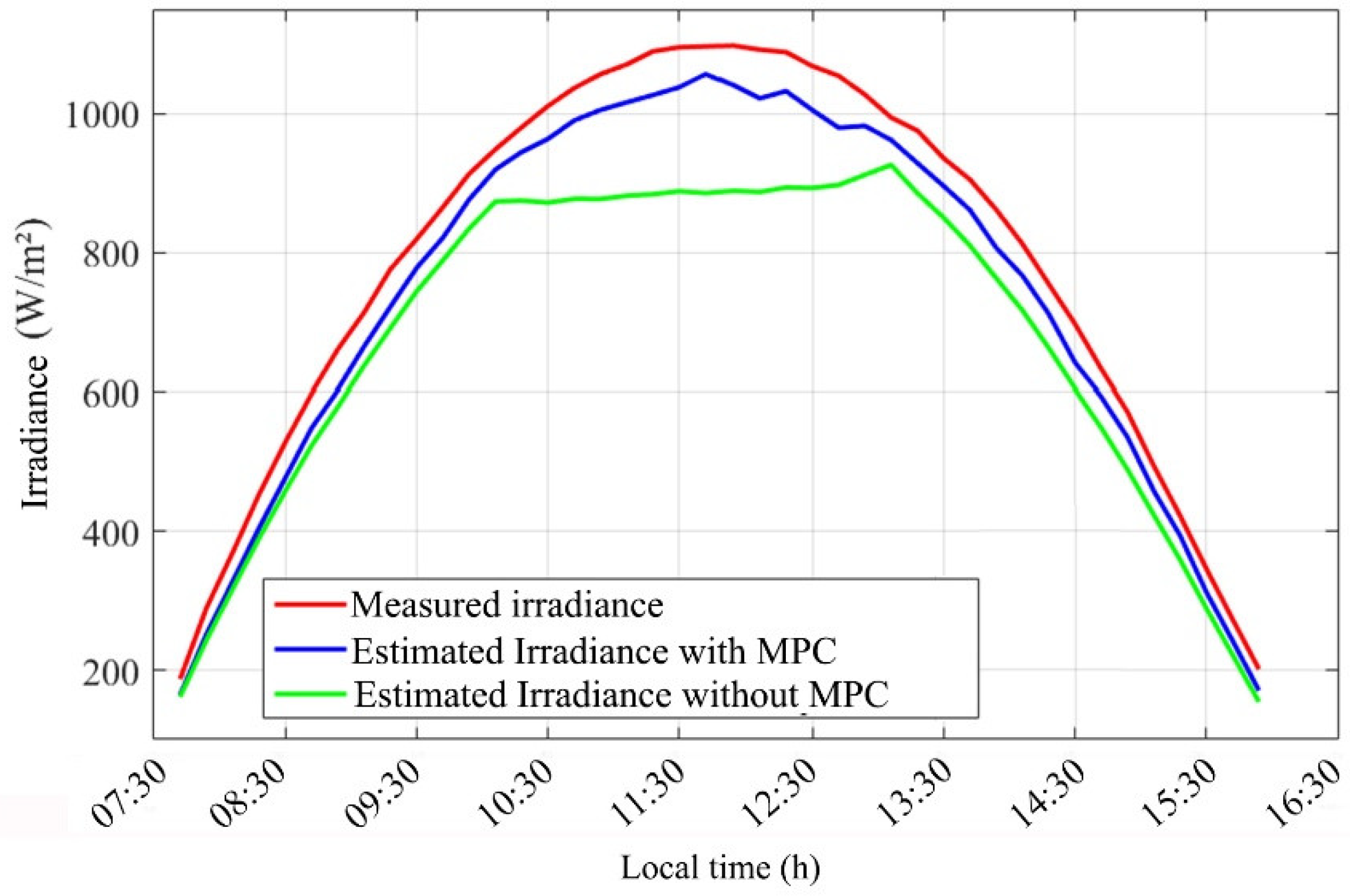
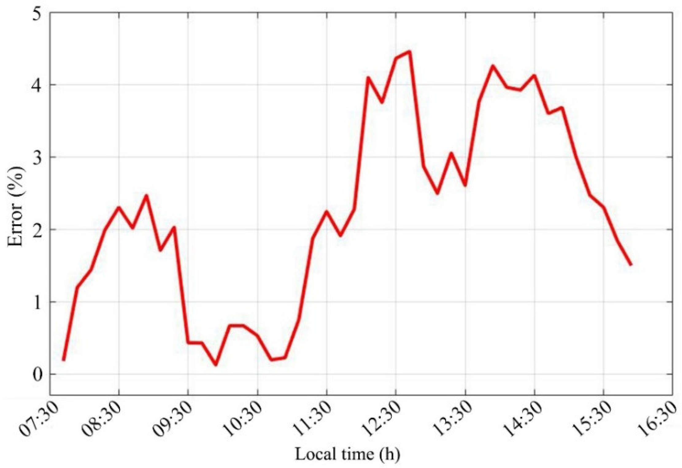
Figure 9 shows the irradiance values obtained from the radiometer (red line), the irradiance estimated by the prototype MPC (blue line) and the irradiance calculated mathematically, without correction. Figure 10 shows the relative error between the measured and estimated irradiance. Figure 9, Figure 10 and Figure 11 present the measurements according to the local time, with the first measurement taking place shortly after 7:30 a.m. and the last measurement around 4:00 p.m.

Once the irradiance used by the modules (G_ac) is defined in (6), the estimation system calculates the available electrical power, that is, the power that the electrical system should have demanded from the photovoltaic modules. The goal is to identify the losses due to dirt and the losses resulting from incompatibilities that may exist from the electrical system of the generation unit.

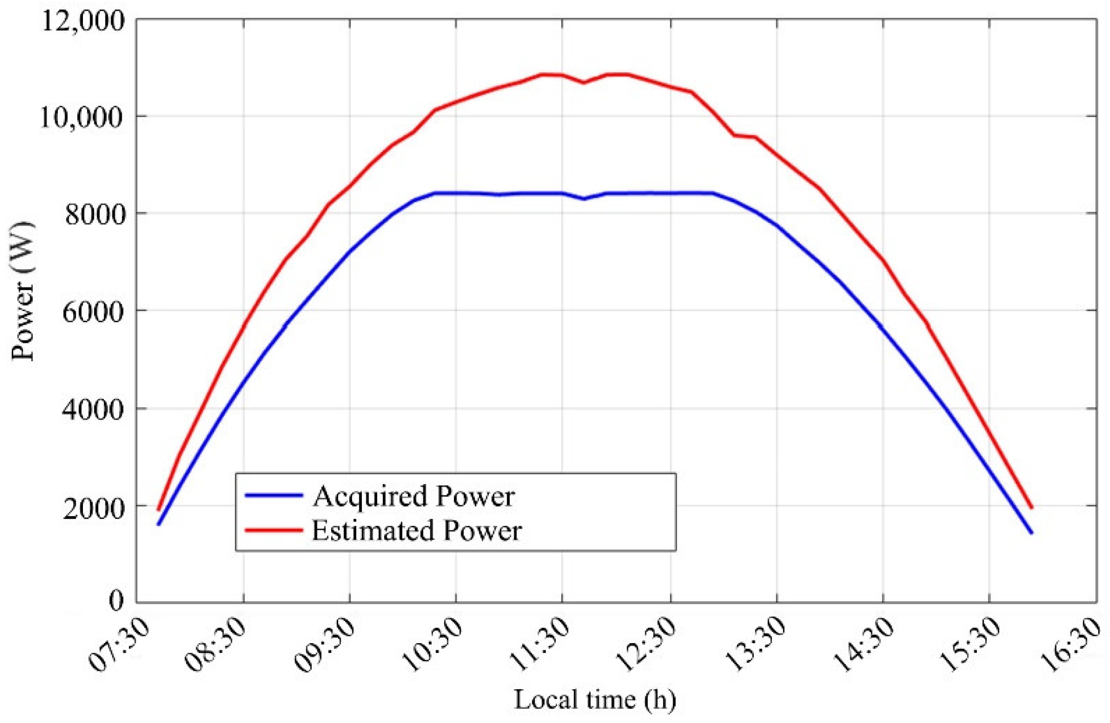
The graph in Figure 11 presents the power reported by the inverter (blue line) and the power calculated by the MPC estimator.

Under normal operating conditions, the power from the inverter should have the same behavior as the estimated power. Once there are differences between both powers, the conclusion is that there may be electrical losses in the system (in this case, losses due to incompatibility between PV system power and maximum inverter power). It is also noteworthy that the estimated peak power is compatible with the solar zenith irradiance on the day of the test (1075 W/m²), reaching 11 kW.

After analyzing the losses results from the experiment, the average daily losses due to dirt were about 4.95%, and the average daily losses due to incompatibility were 15.68%, resulting in a total loss of 20.63%.

It is also worth mentioning the performance of the MPC correcting the values of the series resistance of the solar cells. As seen in Figure 9, the green line represents the calculated irradiance without correction of R_s, where the effects of the inverter saturation appear characterized by the curve flattening. The blue line represents the estimated irradiance with the corrected values of R_s by MPC. One may observe that the line is quite akin to the line of the solar irradiance measured by the radiometer, demonstrating the effectiveness of the MPC estimator.

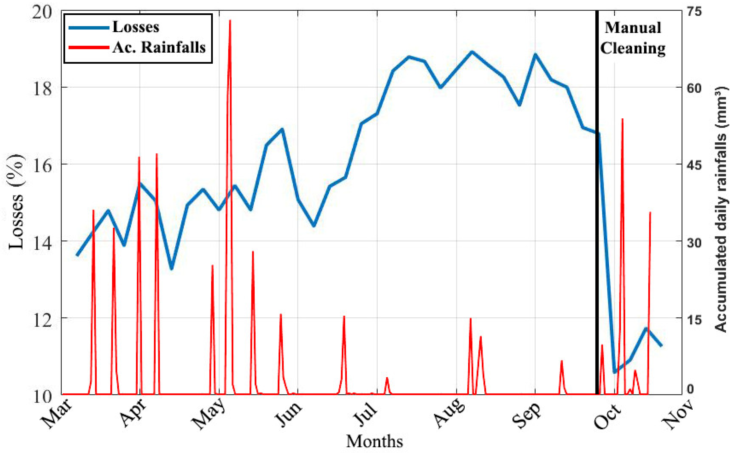
The performance of the predictive model removed the effects of the disturbance out of the electrical system configuration, presenting only the irradiance that effectively affected the photovoltaic cells of the modules. Comparing the estimated and measured irradiances, the dirt losses were 4.95%, free from the problem arisen by the MPPT tracking and the electrical anomalies of the generation system due to incompatibility between the system and the inverter. Figure 12 presents the daily dirt losses and the daily rainfalls from March to October 2019. Losses are around 15% between March and June, most likely due to the location of the system and the low rainfall in the period.

There is a remarkable increase in dirt losses from July to September (around 18%), as the rains were very low during this period. In July, there was only 4 mm of rain, on 26 August mm and on 7 September mm, in the PV plant location. A manual cleaning procedure on the modules was carried out on 27 September, which caused the losses to be reduced sharply on the following day. From additional experiments using a particle sensor along the period of experiments, there were fine particles (particles with diameters between 1 µm and 10 µm) suspended in air, and they may be one impact factor to the dirt on the modules.

4. Conclusions

This work proposed an MPC system to dirt losses estimates and identifying electrical anomalies in photovoltaic power plants. The MPC system receives energy production data from the inverter and irradiation data from a solarimetric station. The losses estimation is based on the difference between the measured irradiance and the estimated irradiance

We have evaluated the MPC estimator for a period of 8 months (March to October/2019). The system estimated losses are 15% between March and June. From July to September, the losses increased to 18% as the rains were very low during this period. Those results reveal that the dirt was determinant to the energy losses in the PV power plant.

The MPC estimator device prototype operates as a power monitoring system, presenting to the administrator the estimation of losses due to dirt and electrical losses. The device has a Wi-Fi communication system that sends real-time information to a supervisory software enabling the administrator to know any anomalies and make decisions regarding the cleaning and maintenance of the modules. Additionally, an administrator can monitor the energy effectively generated by the system and compare it to the energy generation expected by the system. This prototype aims to meet a demand in the photovoltaic solar energy market that lacks similar monitoring solutions, meeting demands from small microgeneration units to large units.

As a future work, the MPC system and its properties can also be applied to control the power converter to optimize energy harvesting as an MPPT algorithm improvement and/or for increasing current controllers stability and robustness of the converter.

References

- ANEEL. Standard 482. pp. 1–13. Available online: http://www2.aneel.gov.br/cedoc/ren2012482.pdf (accessed on 10 March 2020).
- Pinho, J.T.; Galdino, M.A. Engineering Manual for Photovoltaic Systems, 3rd ed.; CEPEL-CRECESB: Rio de Janeiro, Brazil, 2014; 530p. [Google Scholar]
- IRENA—International Renewable Energy Agency. Future of Solar Photovoltaic: Deployment, Investment, Technology, Grid Integration and Socio-Economic Aspects; IRENA: Abu Dhabi, United Arab Emirates, 2019; pp. 1–73. [Google Scholar]
- Durgadevi, A.; Arulselvi, S.; Natarajan, S. Photovoltaic modeling and its characteristics. In Proceedings of the 2011 International Conference on Emerging Trends in Electrical and Computer Technology, Nagercoli, India, 23–24 March 2011; pp. 1–12. [Google Scholar]
- Sayyah, A.; Horenstein, M.N.; Mazumder, M.K. Energy yield loss caused by dust deposition on photovoltaic panels. Sol. Energy 2014, 107, 576–604. [Google Scholar] [CrossRef]
- Karmouch, R.; Hor, H.E.L. Solar Cells Performance Reduction under the Effect of Dust in Jazan Region. J. Fundam. Renew. Energy Appl. 2017, 7, 228. [Google Scholar] [CrossRef]
- Costa, S.C.; Diniz, A.S.A.; Kazmerski, L.L. Dust and soiling issues and impacts relating to solar energy systems: Literature review update for 2012–2015. Renew. Sustain. Energy Rev. 2016, 63, 33–61. [Google Scholar] [CrossRef] [Green Version]
- Sulaiman, S.A.; Singh, A.K.; Mokhtar, M.M.M.; Bou-Rabee, M.A. Influence of Dirt Accumulation on Performance of PV Panels. Energy Procedia 2014, 50, 50–56. [Google Scholar] [CrossRef] [Green Version]
- Saiz, C.S.; Martínez, J.P.; Chivelet, N.M. Influence of Pollen on Solar Photovoltaic Energy: Literature Review and Experimental Testing with Pollen. Appl. Sci. 2020, 10, 4733. [Google Scholar] [CrossRef]
- Martin, N.; Ruíz, J.M. A new model for PV modules angular losses under field conditions. Int. J. Sol. Energy 2002, 22, 19–31. [Google Scholar] [CrossRef]
- Javed, W.; Guo, B.; Figgis, B. Modeling of photovoltaic soiling loss as a function of environmental variables. Sol. Energy 2017, 157, 397–407. [Google Scholar] [CrossRef]
- Wang, L. Model Predictive Control System Design and Implemantation Using Matlab; Springer: Berlin/Heidelberg, Germany, 2009; Volume 1. [Google Scholar]
- Ricker, N.L. Model-predictive control: State of the art. In Proceedings of the Fourth International Conference on Chemical Process Control, Padre Island, TX, USA, 17–22 February 1991; pp. 3–6. [Google Scholar]
- Casaro, M.M.; Martins, D.C. Photovoltaic Array Model Aimed to Analyses in Power Electronics Through Simulation. Eletrôn. Potencia 2008, 13, 141–146. [Google Scholar] [CrossRef]
- Elgohary, R.; Abu ElEla, A.A.; Elkholy, A. Electrical Characteristics Modeling for Photovoltaic Modules Based on Single and Two Diode Models. In Proceedings of the 2018 Twentieth International Middle East Power Systems Conference (MEPCON), Cairo, Egypt, 18–20 December 2018; pp. 685–688. [Google Scholar] [CrossRef]
- Hejri, M.; Mokhtari, H.; Azizian, M.R.; Ghandhari, M.; Soder, L. On the Parameter Extraction of a Five-Parameter Double-Diode Model of Photovoltaic Cells and Modules. IEEE J. Photovolt. 2014, 4, 915–923. [Google Scholar] [CrossRef]
Figure 1.
Irradiance losses in the module surface. (1) Frontal glass; (2) photovoltaic cells; (3) frame.
Figure 2.
Four parameters cell model.
Figure 3.
Effect of the variation of Rs and Rp variation to the I–V curve.
Figure 4.
MPC control block diagram.
Figure 5.
Step response. (a) Experimental setup; (b) oscilloscope waveform response (scales: current 1 A/div; time 10 μs/div).
Figure 6.
MPC losses estimator.
Figure 7.
Comparison of losses using the system with MPC estimation. Estimated losses (in blue); real losses (in green).
Figure 8.
Losses estimator device installed into the PV power plant.
Figure 9.
Incident and estimated solar irradiance, without and with MPC.
Figure 10.
Error between the incident and estimated solar irradiance.
Figure 11.
Comparison between acquired and estimated powers.
Figure 12.
Dirt losses and accumulated daily rainfalls in the UFV-UFMS power plant from March to November 2019.