Fast, Robust, and Low-Cost Microwave Imaging of Multiple Non-Metallic Pipes

Abstract

The use of non-metallic pipes and composite components that are low-cost, durable, light-weight, and resilient to corrosion is growing rapidly in various industrial sectors such as oil and gas industries in the form of non-metallic composite pipes. While these components are still prone to damages, traditional non-destructive testing (NDT) techniques such as eddy current technique and magnetic flux leakage technique cannot be utilized for inspection of these components. Microwave imaging can fill this gap as a favorable technique to perform inspection of non-metallic pipes. Holographic microwave imaging techniques are fast and robust and have been successfully employed in applications such as airport security screening and underground imaging. Here, we extend the use of holographic microwave imaging to inspection of multiple concentric pipes. To increase the speed of data acquisition, we utilize antenna arrays along the azimuthal direction in a cylindrical setup. A parametric study and demonstration of the performance of the proposed imaging system will be provided.

1. Introduction

Currently, non-metallic pipes and composite components such as fiber-reinforced plastic (FRP), glass-reinforced epoxy resin (GRE), high-density polyethylene (HDPE), reinforced rubber expansion joints (REJs), carbon fiber-reinforced plastic (CFRP), and polyvinyl chloride (PVC) are taking over metallic pipes and components due to advantages such as durability, low cost, light weight, resistance to corrosion, etc. Thus, the growing use of these components requires the development of proper non-destructive testing (NDT) techniques for inspection of such materials.

Traditional NDT techniques like ultrasonic testing, eddy current, radiography, and magnetic flux leakage cannot be used to fulfill the evaluation of certain materials such as non-metallic pipes due to various reasons. For instance, ultrasonic testing [1,2] is not suitable to be used for FRP/GRE [3] pipes due to their complex structure of composite materials. Additionally, ultrasonic testing is not suitable for inspection of HDPE thermal fusion joints due to the nature of defects and failure morphology [4,5].

Microwave testing can be used as an NDT technique for inspection of material integrity and condition monitoring. For a more detailed review of microwave NDT methods and applications, please refer to [6,7,8,9]. With the increasing demand for NDT of non-metallic pipes, microwave imaging has been proposed to inspect defects, cracks, and discontinuities in such components [10,11,12,13,14,15,16,17,18]. Recently, holographic microwave imaging has been employed for these applications. Holographic microwave imaging is known to be a fast, robust, and low-cost technique that has been applied in various industrial sectors such as security screening of passengers at airports [19]. In particular, holographic imaging techniques based on synthetic aperture radar (SAR) concepts have been widely studied for non-metallic pipe inspections [19]. Initially, wide-band SAR imaging technique was applied for producing three-dimensional (3D) images of vertical cracks/flaws in HDPE pipes [15]. However, these SAR-based techniques use far-field assumptions, which impose imaging errors for NDT of the pipes. Thus, these techniques were later modified and applied for near-field imaging of non-metallic pipes [20]. This has been accomplished by employing the information related to a specific imaging system a priori through the measurement of point-spread functions (PSFs) [21]. To elaborate further on this issue, in the original holographic imaging techniques [19,22], far-field assumptions, point-wise antennas, and exact background properties were employed to derive the image reconstruction algorithms. However, in the recently proposed near-field holographic imaging techniques [21], it has been shown that the product of the incident field and the Green’s function can be obtained by measuring the PSFs of the imaging system. Thus, due to directly measuring the PSF information using the utilized antennas, the use of near-field holographic imaging reduces different types of errors such as modeling errors, errors due to uncertainties in the material properties, and errors due to the size of antennas. In [20], by employing an array of antennas outside or inside double pipes, the narrowest band data (6–8 GHz) were collected via cylindrical apertures and then 2-D images of the defects on the pipes were reconstructed using near-field holographic imaging. The use of narrowband data allows for reducing the errors due to the material’s dispersive properties and lowering the cost and complexity of the imaging system [20,23,24]. Thus, to have a low-cost system for holographic microwave imaging, a data acquisition system was built employing off-the-shelf components [24]. Additionally, to expedite the data acquisition process, electronically scanned antennas can replace the mechanical scanning. A practical method is using antenna arrays along one axis and completing the data acquisition by mechanically scanning the array along the orthogonal direction [19,22,25]. In [23], the azimuthal direction ($\varphi$) was electronically scanned via the use of antenna arrays while the longitudinal direction (z) was mechanically scanned using motors. There, three processing methods were compared in terms of performance for limited and non-uniform sampling along the azimuthal direction. Results in [23] showed that near-field holographic imaging using interpolation to produce uniform samples along the azimuthal direction followed by uniform Fourier transform works better than using non-uniform samples and non-uniform Fourier transform for the proposed setup. Another approach to tackle the problem of non-uniform sampling could be the use of an optimal sampling method proposed in [26], which necessitated re-designing the angular distribution of the antennas.

Here, we propose the use of holographic imaging technique with arrays of antennas for inspection of multiple non-metallic pipes. The arrays are along the azimuthal direction ($\varphi$) and they scan the pipes along the longitudinal direction (z). Concentric non-metallic pipes are commonly used in different industrial sectors for various purposes such as protection of production tubes in oil and gas extraction [27] and fluid transfer (to separate different fluids) [28]. The proposed system allows for fast data acquisition, which facilitates the development of a real-time imaging system to inspect long, concentric pipes. Similar to [23], to solve the relevant systems of equations in near-field holographic microwave imaging, we employ interpolation, uniform Fourier transform, and Standardized low-resolution brain electromagnetic tomography (sLORETA). Instead of using a vector network analyzer (VNA), a low-cost and compact imaging system is adapted from [23]. The main contribution of this work is related to the imaging of defects in multiple, non-metallic, concentric pipes and the capabilities and limitations of the relevant microwave imaging system. Due to the multiple scattering of the waves between the two pipes, this is a more challenging imaging problem compared to the one in [23] (imaging of objects in a homogenous background medium). By using antenna arrays, the data acquisition is significantly expedited for longitudinally long structures such as pipelines, which, in turn, leads to faster inspection of such structures. For this purpose, we first study the effect of important parameters such as defect size, number of frequencies, standoff distance of the antennas, and property of the fluids carried by the pipes. Then, we demonstrate the performance of the proposed system through experimental results.

2. Theory

First, we present the holographic near-field microwave imaging for inspection of multiple pipes when using the data acquired by an array of antennas distributed along the azimuthal axis. The imaging algorithm is adapted from [23].

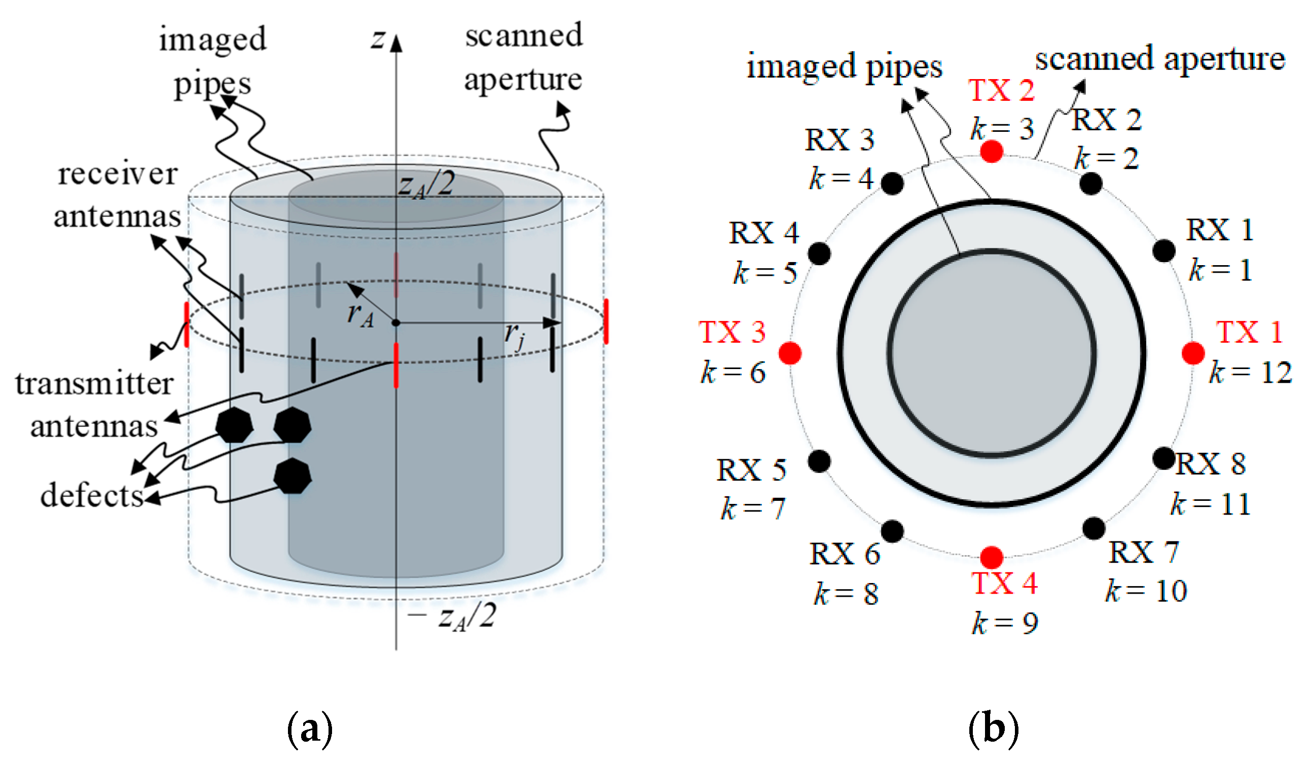
Figure 1 illustrates the imaging setup with the transmitter and receiver antenna arrays for the inspection of double concentric pipes. In this microwave imaging system, N_T transmitter antennas are distributed uniformly along the azimuthal direction with angular separation of $\Delta {\varphi }_T$. Additionally, ${N^{\prime }}_R$ receiver antennas separated by $\Delta {\varphi }_R$ are placed between two consecutive transmitter antennas. Thus, we have $N_R={N^{\prime }}_R\times N_T$ receiver antennas and overall $N_A=N_R+N_T$ antennas uniformly distributed over the azimuthal direction. The scanned cylindrical aperture has a radius of r_A and height of $z_A$. While scanning along the azimuthal direction is implemented electronically using the utilized antenna arrays, scanning along the longitudinal direction (at multiple heights $z_l$, $l=1,\dots ,N_z$) is implemented by mechanically moving the antenna array and collecting data at frequencies ${\omega }_n$ within the band of ${\omega }_1$ to ${\omega }_{N_{\omega }}.$ The number of imaged pipes is denoted by $N_r$ and the pipes have radii of $r_j$, $j=1,\dots ,N_r$.

Commonly, in near-field microwave holographic imaging techniques, the imaging system is assumed to be linear and space invariant (LSI). Thus, as a first step, point-spread functions (PSFs) of the imaging system are collected for each imaged pipe. This is implemented by placing a small defect, called calibration defect (CD), on each pipe j and measuring the scattered responses $E_{j,a_m}^{SC,CD}({\varphi }_{k^{\prime }},z_l,{\omega }_n)$ for each illuminating transmitter a_m and each measurement frequency ${\omega }_n$ (where $n=1,\dots ,N_{\omega }$) and received by all receiver antennas at angles of ${\varphi }_{k^{\prime }}$ (where $k^{\prime }=1,\dots ,N_R$). In practice, CDs are the smallest measurable defects on each imaged pipe, representing an impulse function input to the LSI imaging system.

For the test scenario, the scattered response $E_{a_m}^{SC}({\varphi }_{k^{\prime }},z_l,{\omega }_n)$ for all defects on all the pipes is excited by each transmitter a_m and recorded by all receiver antennas at all frequencies ${\omega }_n$. Since the collected responses $E_{j,a_m}^{SC,CD}({\varphi }_{k^{\prime }},z_l,{\omega }_n)$ and $E_{a_m}^{SC}({\varphi }_{k^{\prime }},z_l,{\omega }_n)$ ($k^{\prime }=1,\dots ,N_R$) are non-uniform along the azimuthal direction, first, interpolation is employed to obtain responses $E_{j,a_m}^{SC,CD}({\varphi }_k,z_l,{\omega }_n)$ and $E_{a_m}^{SC}({\varphi }_k,z_l,{\omega }_n)$ ($k=1,\dots ,N_A$) that are uniformly distributed along that direction.

When using superposition principle, the interpolated scattered field $E_{a_m}^{SC}({\varphi }_k,z_l,{\omega }_n)$ can be approximated by the sum of the terms $E_{j,a_m}^{SC}({\varphi }_k,z_l,{\omega }_n)$, which are the scattered responses from the defects over each pipe j. Due to the LSI assumption, $E_{j,a_m}^{SC}({\varphi }_k,z_l,{\omega }_n)$ can be, in turn, written as the convolution of the PSF collected for pipe j, $E_{j,a_m}^{SC,CD}({\varphi }_k,z_l,{\omega }_n)$, with the shape function of the defects for the corresponding pipe $f_j({\varphi }_k,z_l)$. According to the abovementioned approximations, $E_{a_m}^{SC}({\varphi }_k,z_l,{\omega }_n)$ is written as:

$$E_{a_m}^{SC}({\varphi }_k,z_l,{\omega }_n)={\displaystyle \sum _{j=1}^{Nr}{E}_{j,a_m}^{SC}({\varphi }_k,z_l,{\omega }_n)}={\displaystyle \sum _{j=1}^{Nr}{E}_{j,a_m}^{SC,CD}({\varphi }_k,z_l,{\omega }_n)}{\ast }_{\varphi }{\ast }_z{f}_j({\varphi }_k,z_l)$$

(1)

where ${\ast }_{\varphi }$ and ${\ast }_z$ denote the convolutions along the azimuthal ($\varphi$) and longitudinal (z) directions. In [21], it was shown that the shape function $f_j({\varphi }_k,z_l)$ is related to the contrast in dielectric properties with respect to the background medium, assuming that such contrast is independent of the frequency over a narrow band. Writing Equation (1) at all measurement frequencies ${\omega }_n$, $n=1,\dots ,N_{\omega }$, we obtain the following system of equations:

$$\{\begin{array}{c}{E}_{a_m}^{SC}({\varphi }_k,z_l,{\omega }_1)={\displaystyle \sum _{j=1}^{N_r}{E}_{j,a_m}^{SC,CD}D({\varphi }_k,z_l,{\omega }_1){\ast }_{\varphi }{\ast }_z{f}_j({\varphi }_k,z_l)}\\ ⋮\\ E_{a_m}^{SC}({\varphi }_k,z_l,{\omega }_{N_{\omega }})={\displaystyle \sum _{j=1}^{N_r}{E}_{j,a_m}^{SC,CD}({\varphi }_k,z_l,{\omega }_{N_{\omega }}){\ast }_{\varphi }{\ast }_z{f}_j({\varphi }_k,z_l)}\end{array}$$

(2)

By applying discrete-time Fourier transform (DTFT) along z and discrete Fourier transform (DFT) along $\varphi$ to both sides of the equations in Equation (2), the following system of equations are obtained at each spatial frequency pair $\mathit{\kappa }=(k_{\varphi },k_z)$ (where $k_{\varphi }$ and $k_z$ are Fourier variables corresponding to $\varphi$ and z variables, respectively):

$$\{\begin{array}{c}{\stackrel{\widetilde{˜}}{\mathbf{E}}}_{a_m}^{SC}(\mathit{\kappa },{\omega }_1)={\displaystyle \sum _{j=1}^{N_r}{\stackrel{\widetilde{˜}}{\mathbf{E}}}_{j,a_m}^{SC,CD}(\mathit{\kappa },{\omega }_1){\stackrel{\widetilde{˜}}{\mathrm{f}}}_j(\mathit{\kappa })}\\ ⋮\\ {\stackrel{\widetilde{˜}}{\mathbf{E}}}_{a_m}^{SC}(\mathit{\kappa },{\omega }_{N_{\omega }})={\displaystyle \sum _{j=1}^{N_r}{\stackrel{\widetilde{˜}}{\mathbf{E}}}_{j,a_m}^{SC,CD}(\mathit{\kappa },{\omega }_{N_{\omega }}){\stackrel{\widetilde{˜}}{\mathrm{f}}}_j(\mathit{\kappa })}\end{array}$$

(3)

where ${\stackrel{\widetilde{˜}}{\mathbf{E}}}_{a_m}^{SC}(\mathit{\kappa },{\omega }_n)$, ${\stackrel{\widetilde{˜}}{\mathbf{E}}}_{j,a_m}^{SC,CD}(\mathit{\kappa },{\omega }_n)$, and ${\stackrel{\widetilde{˜}}{\mathrm{f}}}_j(\mathit{\kappa })$ are functions after taking DFT along $\varphi$ and DTFT along z axis of $E_{a_m}^{SC}({\varphi }_k,z_l,{\omega }_n)$, $E_{j,a_m}^{SC,CD}({\varphi }_k,z_l,{\omega }_n)$, and $f_j({\varphi }_k,z_l)$, respectively. The DTFT along $\varphi$ reduces to DFT due to the periodicity of the functions along that direction.

By writing Equation (3) for all N_T transmitters, a system of equations with shared unknown parameters ${\stackrel{\widetilde{˜}}{\mathrm{f}}}_j(\mathit{\kappa })$ is obtained at each spatial frequency pair $\mathit{\kappa }=(k_{\varphi },k_z)$ as:

$${\tilde{\widetilde{\underset{\_}{\mathbf{E}}}}}^{SC}=\tilde{\tilde{\underset{\_}{\underset{\_}{\mathbf{D}}}}}\tilde{\widetilde{\underset{\_}{\mathbf{F}}}}$$

(4)

where

$${\tilde{\widetilde{\underset{\_}{\mathbf{E}}}}}^{SC}=\left[\begin{array}{c}{\tilde{\widetilde{\underset{\_}{\mathbf{E}}}}}_1^{SC}\\ ⋮\\ {\tilde{\widetilde{\underset{\_}{\mathbf{E}}}}}_{N_T}^{SC}\end{array}\right], \underset{\_}{\tilde{\widetilde{\underset{\_}{\mathbf{D}}}}}=\left[\begin{array}{c}{\tilde{\widetilde{\underset{\_}{\mathbf{D}}}}}_1\\ ⋮\\ {\tilde{\widetilde{\underset{\_}{\mathbf{D}}}}}_{N_T}\end{array}\right], \tilde{\widetilde{\underset{\_}{\mathbf{F}}}}=\left[\begin{array}{c}{\widetilde{\tilde{\mathrm{f}}}}_1(\mathit{\kappa })\\ ⋮\\ {\widetilde{\tilde{\mathrm{f}}}}_{N_r}(\mathit{\kappa })\end{array}\right]$$

(5)

and

$${\tilde{\widetilde{\underset{\_}{\mathbf{E}}}}}_{a_m}^{SC}=\left[\begin{array}{c}{\widetilde{\tilde{\mathbf{E}}}}_{a_m}^{SC}(\mathit{\kappa },{\omega }_1)\\ ⋮\\ {\widetilde{\tilde{\mathbf{E}}}}_{a_m}^{SC}(\mathit{\kappa },{\omega }_{N_{\omega }})\end{array}\right]$$

(6)

$${\underset{\_}{\widetilde{\tilde{\mathbf{D}}}}}_{a_m}=\left[\begin{array}{ccc}{\widetilde{\tilde{\mathbf{E}}}}_{1,a_m}^{SC,CD}(\mathit{\kappa },{\omega }_1)& \cdots & {\widetilde{\tilde{\mathbf{E}}}}_{N_r,a_m}^{SC,CD}(\mathit{\kappa },{\omega }_1)\\ ⋮& \ddots & ⋮\\ {\widetilde{\tilde{\mathbf{E}}}}_{1,a_m}^{SC,CD}(\mathit{\kappa },{\omega }_{N_{\omega }})& \cdots & {\widetilde{\tilde{\mathbf{E}}}}_{N_r,a_m}^{SC,CD}(\mathit{\kappa },{\omega }_{N_{\omega }})\end{array}\right]$$

(7)

Such system of equations is solved using the sLORETA approach (for details please refer to [23]) at each $\mathit{\kappa }=(k_{\varphi },k_z)$ pair to obtain the values for ${\widetilde{\tilde{\mathrm{f}}}}_j(\mathit{\kappa })$, $j=1,\dots ,N_r$. Then, inverse DTFT along z and inverse DFT along $\varphi$ are applied to reconstruct images $f_j({\varphi }_k,z_l)$ over all the surfaces with radii $r=r_j$, $j=1,\dots ,N_r$. At the end, the normalized modulus of $f_j({\varphi }_k,z_l)$, $|f_j({\varphi }_k,z_l)|/M$ (called normalized image), where $M$ is the maximum of $|f_j({\varphi }_k,z_l)|$ for all $r_j$, is plotted to obtain a two-dimensional (2D) image of each pipe.

3. Simulation Results

In this section, we validate the performance of the proposed imaging technique via FEKO simulations for inspection of double concentric pipes.

3.1. Parametric Study

Here, we present the study of the effect of important parameters on the proposed imaging technique. To expedite the study, we assume that the pipes and their defects are infinite along the longitudinal (z) direction. Thus, we evaluate the performance using one-dimensional (1D) images for each pipe. The operating frequency of the proposed setup is from 1.5 GHz to 1.9 GHz (centering at 1.7 GHz). Selection of this frequency range allows for a compromise between resolution and penetration depth for lossy liquids carried inside the pipes. The liquid between the pipes has a relative permittivity ε_r of 22 and conductivity of 1.25 S/m. These properties are chosen to represent mixtures of water and other liquids such as oil. In addition, it is worth noting that a liquid mixture with higher water content is more dissipative, which hinders penetration of microwave power for inspection.

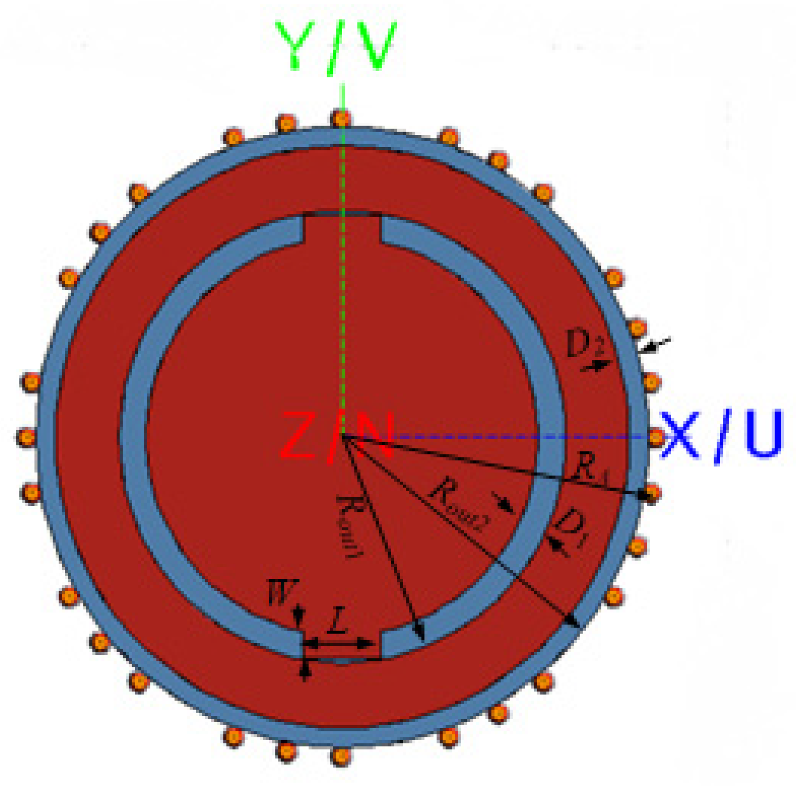
Figure 2 shows the illustration of the reference setup, in which there are two concentric pipes with radii of R_out1 = 57.5 mm and R_out2 = 79 mm. The pipes have thicknesses of D_out1 = 7 mm and D_out2 = 5 mm. There are two defects on the inner pipe centered at $\varphi =$90° and −90°. The defects are with azimuthal arc length of L = 20 mm and radial width of W = 6.8 mm. The pipes have a relative permittivity ε_r of 2.25 and loss tangent of 0.0004 (these properties are close to the properties of PVC material at microwave regime).

An array of 36 half-wavelength dipole antennas with angular separation $\Delta {\varphi }_a$ = 10° was placed at the radius R_a of 81 mm. From these, 27 antennas act as receiver antennas and the rest are transmitter antennas. The sampling frequency step is 0.1 GHz. To have a realistic study, we add white Gaussian noise with signal-to-noise ratio (SNR) of 20 dB to the simulated responses.

To have a quantitative assessment of the reconstructed images, we use structural similarity (SSIM) index [29]. This index is composed of three terms: the luminance term, the contrast term, and the structural term. Here, SSIM is computed for each 1D image by using the true pipe’s image as the reference. The true image has a value of 1 at the pixels overlapping the defect and 0 elsewhere. Higher SSIM values represent higher image reconstruction quality.

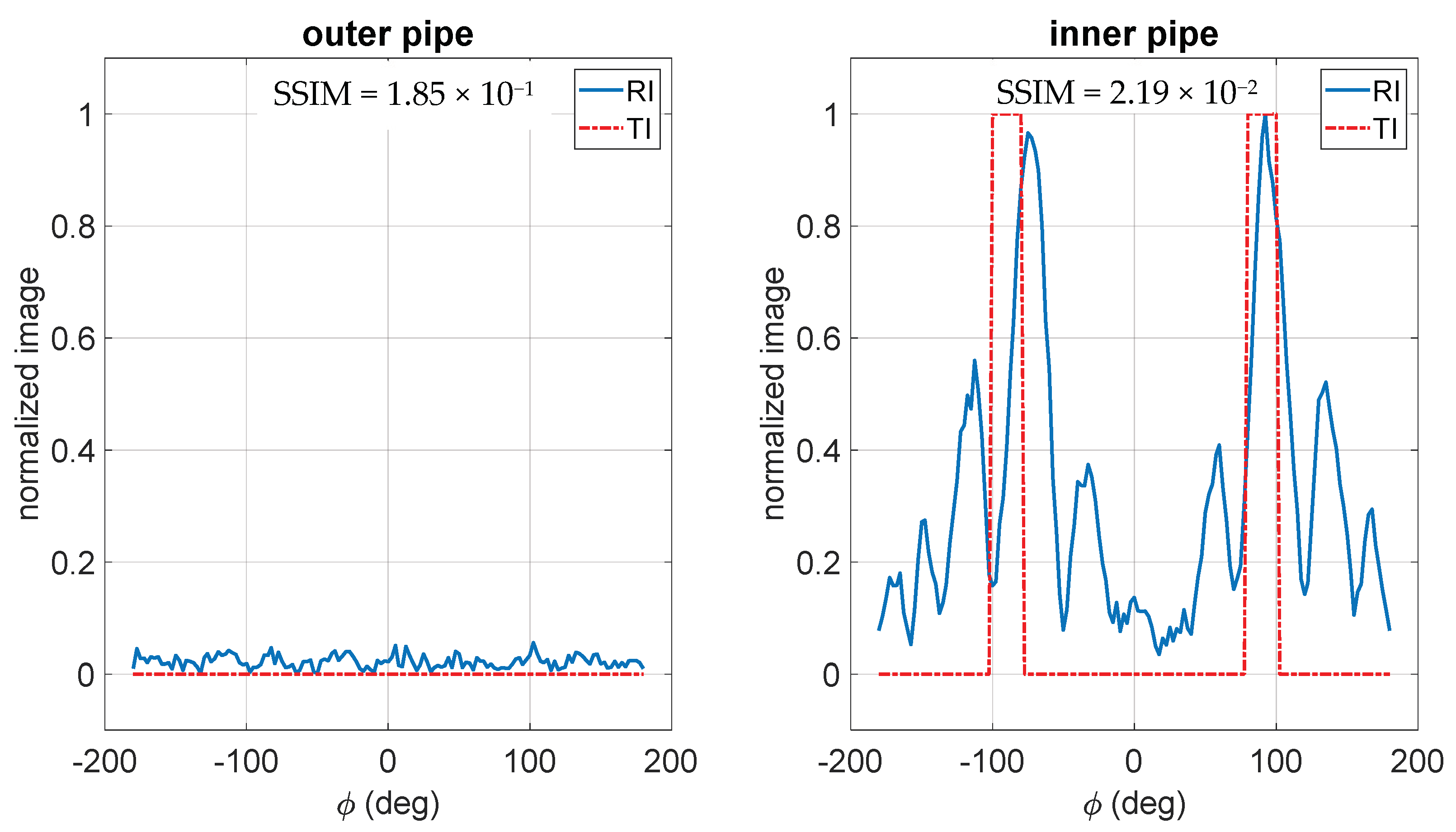
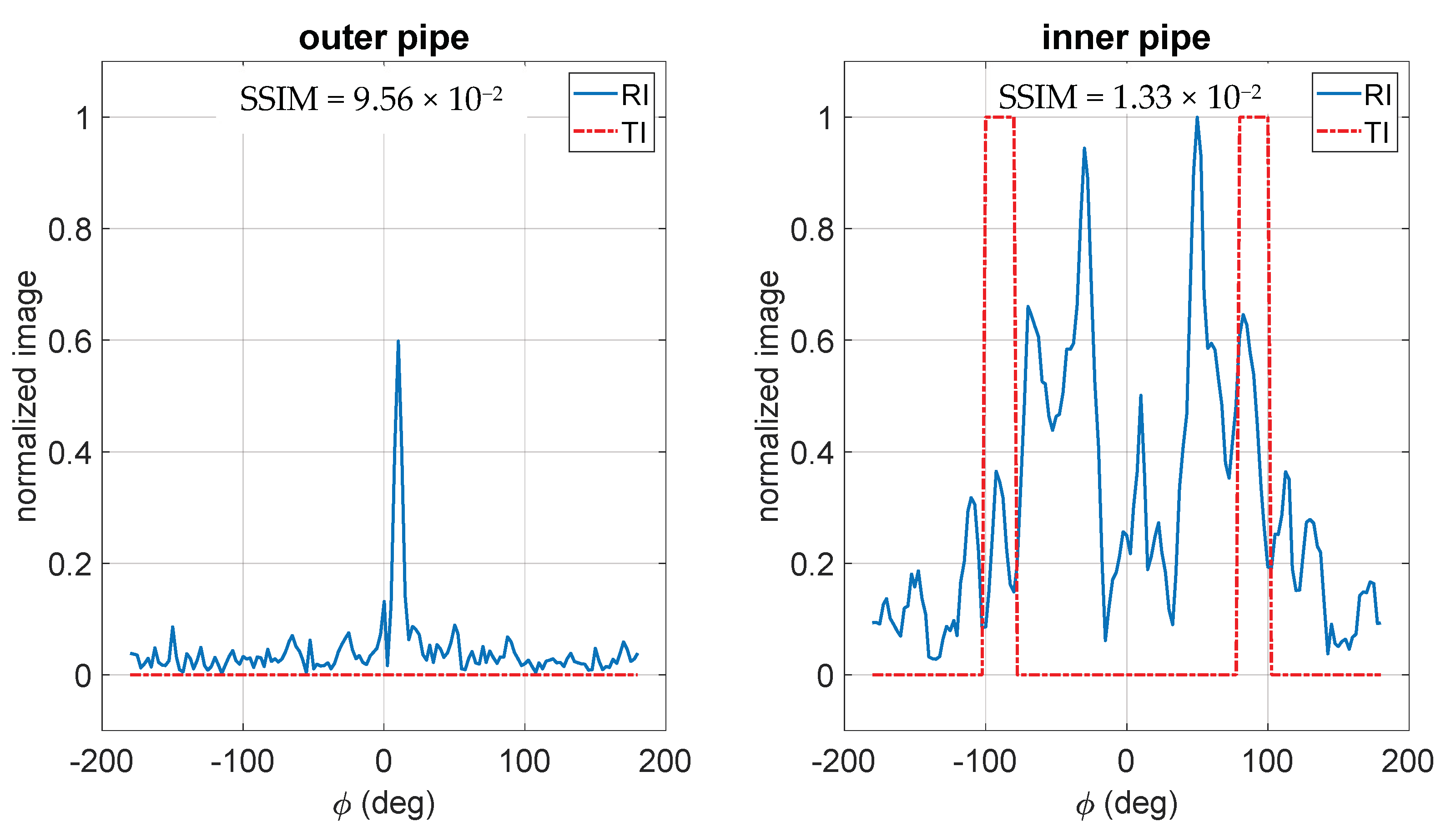
Figure 3 shows the reconstructed images of the reference case. The two defects can be clearly distinguished along with some background artifacts.

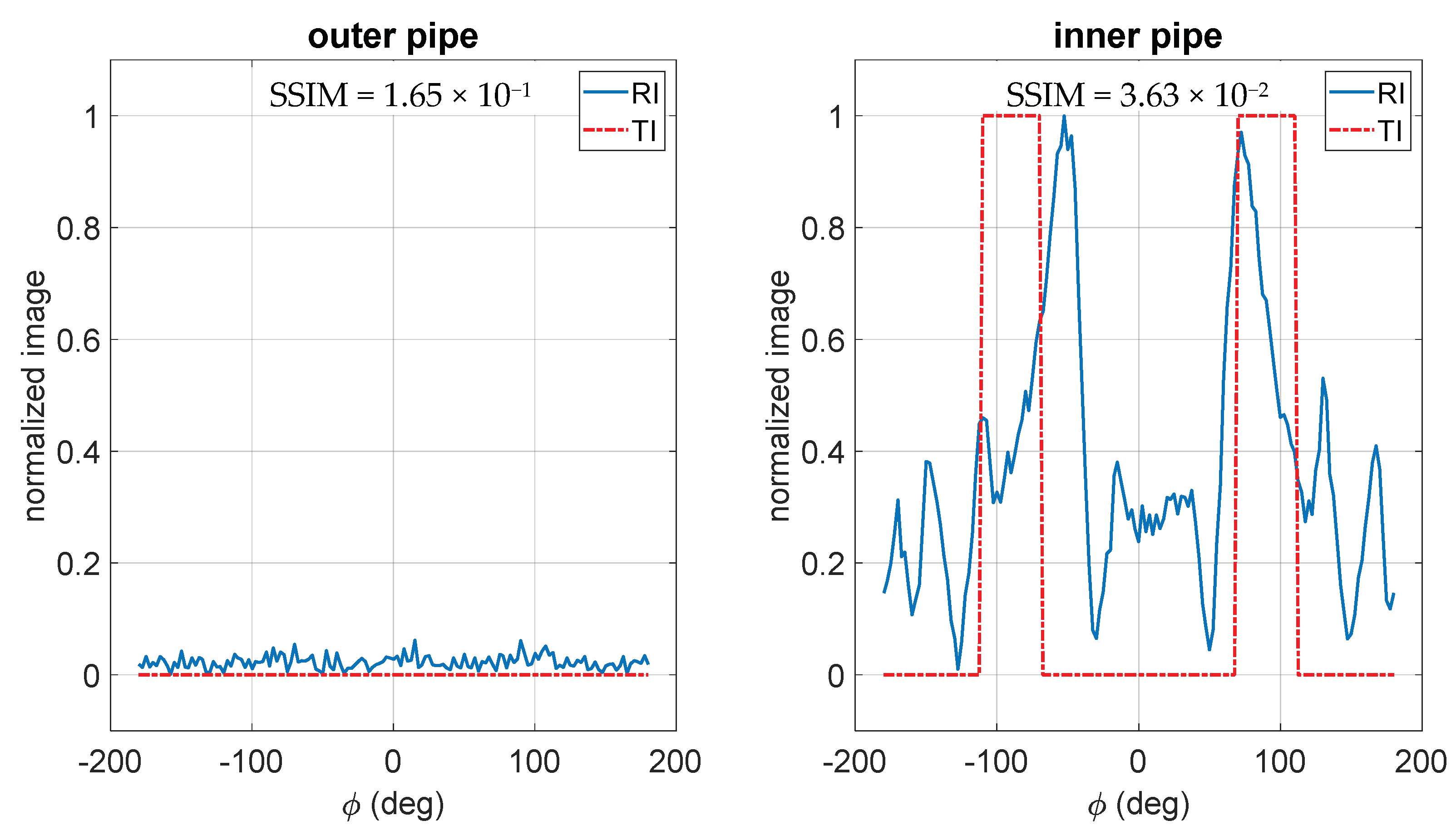
To study the effect of larger defect size, we increased the azimuthal spread of the defect to two times of the original one (L = 40 mm). The reconstructed images are shown in Figure 4. It was observed that with the increase of the defect size, the value of SSIM increased (the quality of reconstructed images improved).

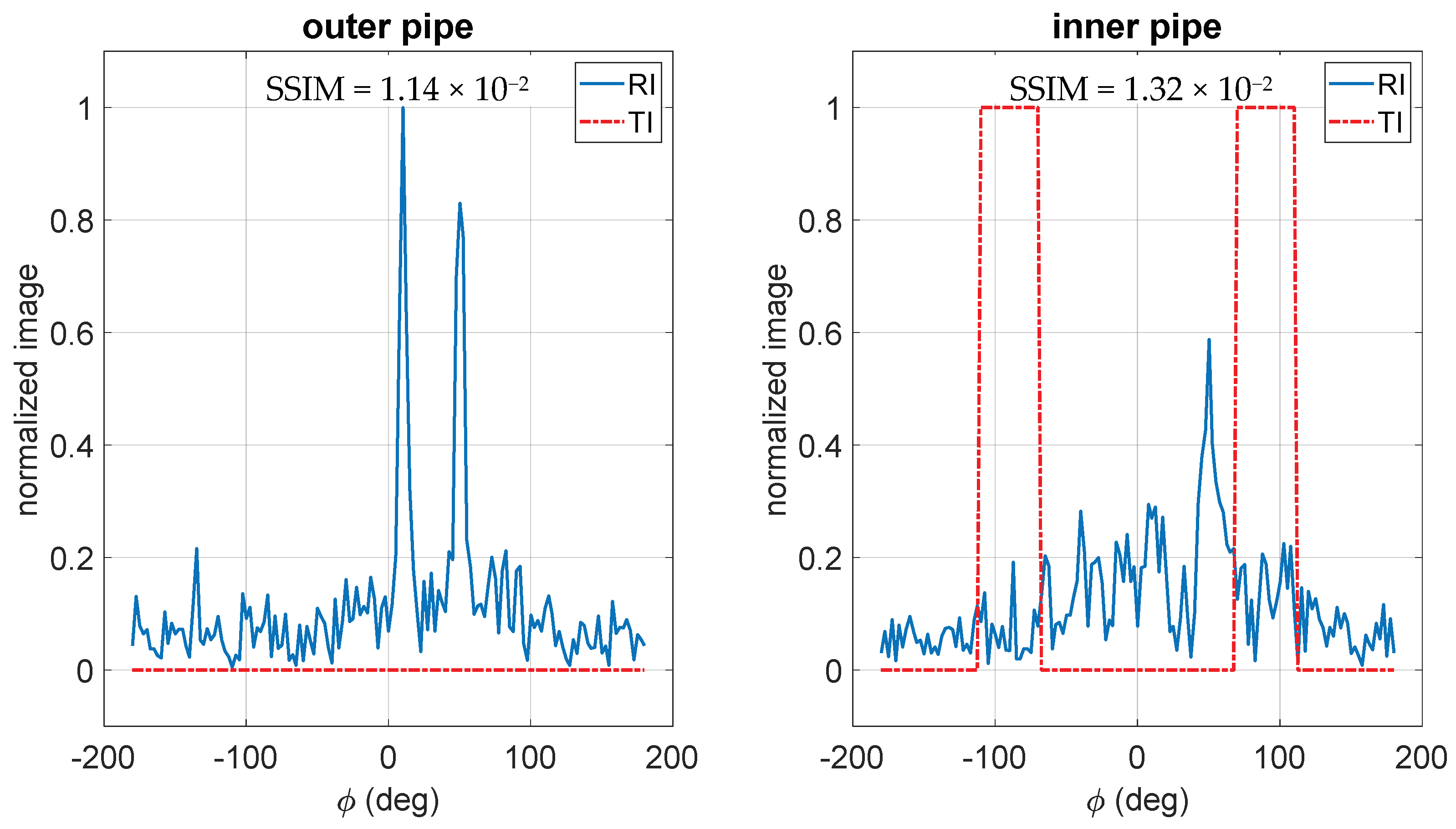
Then, we study the effect of operating frequency. Figure 5 shows the reconstructed images using single frequency data at 1.7 GHz. The use of a single frequency reduces the cost and complexity of the data acquisition system. The background artifacts are higher compared to the reference case due to the insufficient frequency data. This is evident when comparing the SSIM values for the inner pipe’s image in Figure 3 and Figure 5.

To study the effect of standoff distance, we add a standoff distance of 2 mm between the antenna array and the outer pipe (R_a = 83 mm) for the reference setup while we keep using the simulated PSFs for the case when R_a = 81 mm. Figure 6 shows the reconstructed images. The image quality degrades drastically and the two defects cannot be resolved well. The SSIM value is much lower for the inner pipe’s image compared to the reference case in Figure 3.

Next, we study the effect of uncertainty in knowing the exact property of the fluids carried by the pipes. We change the relative permittivity of the inner pipe’s liquid and the outer pipe’s liquid (liquid in between the two pipes) in the reference setup while still using the PSFs collected for the original properties.

Figure 7 shows the reconstructed images of the pipes when the inner pipe’s liquid relative permittivity is 18 while the outer pipe’s liquid permittivity is 22. We use the PSFs collected for the case that the permittivity for both liquids is assumed to be 22. Compared to the reconstructed images of the reference setup in Figure 3, the background artifacts are higher, which leads to a lower SSIM value for the inner pipe’s image. It is observed that when the fluid property is not correct, the image quality degrades.

Figure 8 shows the reconstructed images of the pipes when the relative permittivity of the outer pipe’s liquid is 18 while the permittivity of inner pipe’s liquid is 22. We use the PSFs collected for the case that the permittivity for both liquids is assumed to be 22. It is observed that the defects could not be distinguished at all in this case. By comparing these results with those at Figure 7, we conclude that the imaging results are much more sensitive to uncertainties in knowing the properties of the liquid carried by the outer pipe compared to that of the inner pipe.

3.2. 2D Image Reconstruction for Each Pipe: Simulation Study

In this section, we present the results for imaging of defects on double concentric pipes used in the previous section. All the parameters of the setup for the antenna arrays and the pipes are similar to those shown in Figure 2 except that the length of the pipes is 285 mm along the z axis. Additionally, the data collection is performed over a cylindrical aperture with the length of 260 mm along the z axis. The antenna array scanned the aperture over 19 steps along the z axis. Figure 9 shows the imaging results for the two defects on the inner pipe. The defects can be distinguished well. Similarly, Figure 10 shows the imaging result for the two defects on the outer pipe. The defects can be distinguished well in this case, as well. Comparing the SSIM values, Figure 10 has better image quality compared to Figure 9, as expected due to stronger responses for the defects.

4. Experimental Results

In this section, we present the results when using a low-cost microwave data acquisition system for imaging of double concentric PVC pipes. The operating frequency is from 1.5 GHz to 1.9 GHz (centering at 1.7 GHz).

4.1. Data Acquisition System

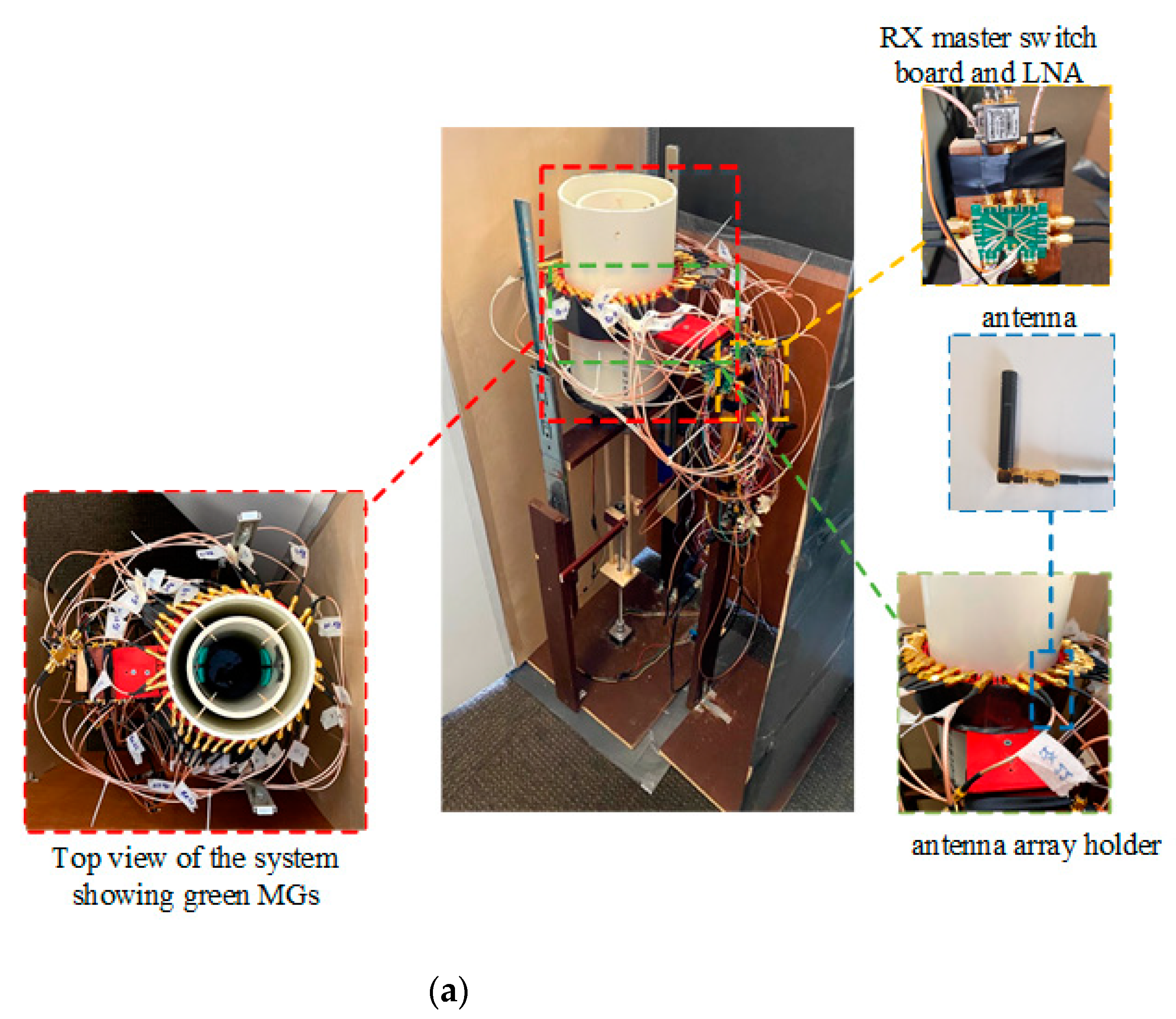
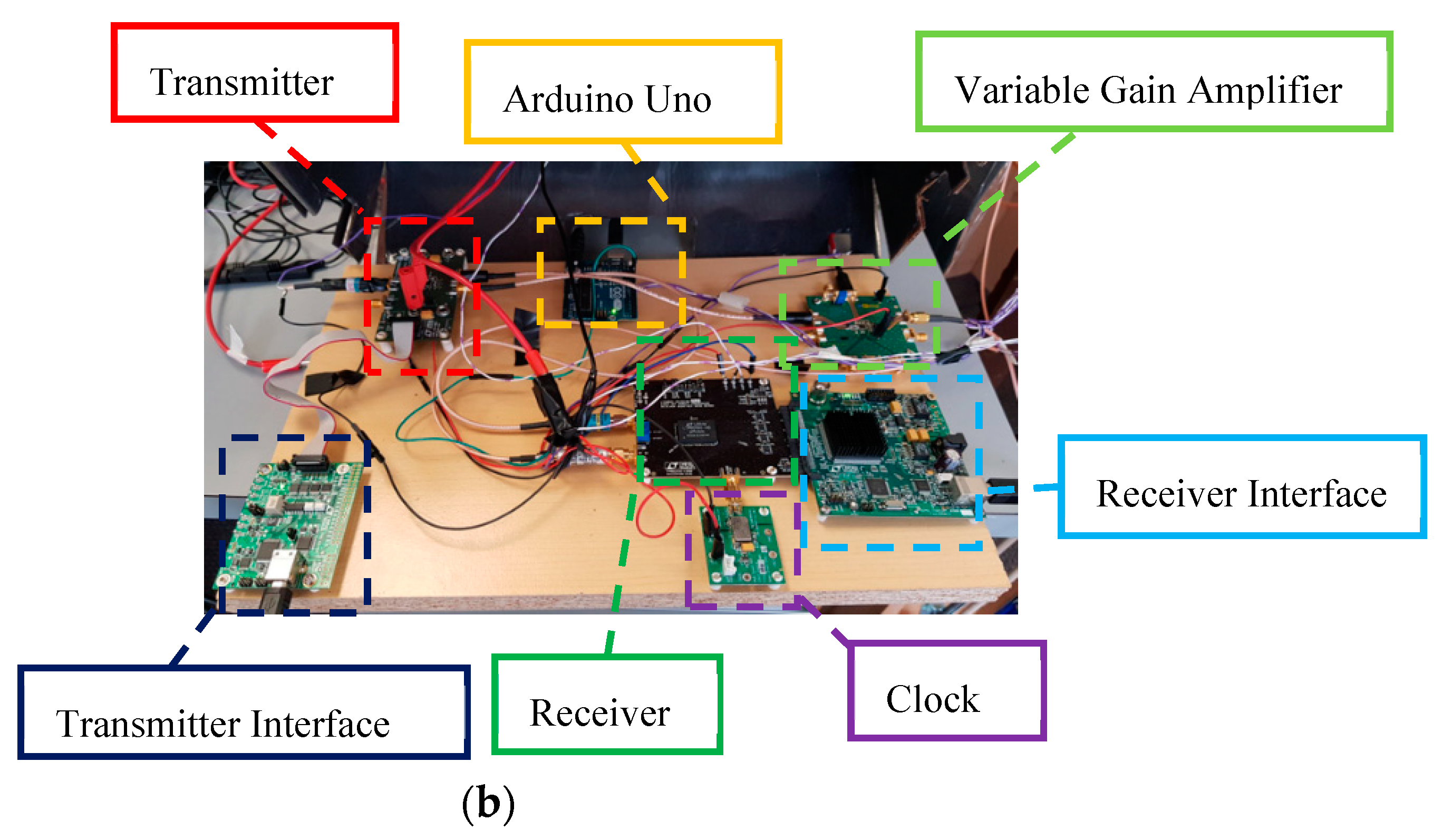
The imaging system consists of microwave boards for transmission and reception of signals, transmitter and receiver antenna arrays, two switching networks for the arrays, a control and processing unit, and a scanning setup, which is adapted from [23]. Figure 11 shows the main components of the experimental setup.

Here, two PVC pipes contain a liquid mixture of 60% water and 40% glycerin with relative permittivity of 62 and conductivity of 2.15 S/m at the operating frequency band [30]. The outer pipe has an inner diameter of 152 mm (6 in), a thickness of 5 mm, and a height of 300 mm. The inner pipe has an inner diameter of 101.6 mm (4 in), a thickness of 7 mm, and a height of 282 mm. For implementation simplicity, we try to image regions of material gains (MGs) instead of material loss (defects) in our experiments. The used MGs are circular-shaped PVC materials with a diameter of 50 mm. During the scan, the system moves the two pipes with liquid mixture along the longitudinal direction (z).

The number and spatial distribution of the antennas are similar to the ones in the simulations, e.g., see Figure 2. The transmitter antennas are separated by $\Delta {\varphi }_T$ = 40°. The adjacent receiver antennas are separated by $\Delta {\varphi }_R$ = 10° (no receiver antennas at the transmitter antennas’ positions). A custom, 3D-printed holder, which consists of 36 circular slots to place the antennas, is made to keep the antennas in close contact with the outer pipe. Additionally, to lower the direct coupling between the adjacent antennas, microwave absorbing sheets are inserted in the 36 slots with widths of 1 mm in between antennas. On the outer surface of the antenna holder, we attach a microwave absorbing sheet to further reduce the interferences. For a fast, proof-of-concept prototype, commercial antennas are used. They are mini GSM/Cellular Quad-Band antennas from Adafruit Company.

The frequency synthesizer is DC1705C-B from Analog Devices, operating from 0.513 GHz to 4.91 GHz, and the direct conversion receiver is DC1513B-AB from Analog Devices, operating from 0.7 GHz to 2.7 GHz. Further details regarding these modules can be found in [24]. In addition, two separate switching networks are built for selecting the transmitter and receiver antennas using EV1HMC321ALP4E modules from Analog Devices. The switching networks are controlled by MATLAB via Arduino Uno boards.

4.2. Experimental 2D Imaging Results for Each Pipe

In this section, we conduct experiments for validating the performance of the proposed imaging system. The operating frequency is from 1.5 GHz to 1.9 GHz with steps of 0.1 GHz (centering at 1.7 GHz). The experiments are implemented on two concentric PVC pipes with MGs either attached on the inner surface of the outer pipe or inner pipe.

We consider two experiments: (1) Two MGs are placed on the inner surface of the outer pipe and (2) two MGs are placed on the inner surface of the inner pipe. For both experiments, data acquisition is implemented electronically along the azimuthal direction and mechanically along the longitudinal direction. Sampling along z axis with 39 steps is performed over a length of 4λ, where λ is the wavelength at 1.7 GHz for the mixture.

For each receiver antenna, the complex-valued, scattered response (R) is composed by using the outputs of in-phase (I) and quadrature (Q) channels for the receiver unit as: R = I + jQ. Here, R depends on the angular position ${\varphi }_{k^{\prime }}$, longitudinal position $z_l$, and frequency ${\omega }_n$. By default, at each data acquisition step, 1024 samples are provided by the receiver unit for each channel. Then, we average the 1024 samples for each channel to acquire I and Q values.

Measurements of PSFs are obtained by using one circular PVC MG with diameter of 50 mm and thickness of 5 mm. The MG is placed inside the outer pipe for the measurement of PSFs corresponding to the outer pipe. Then, the MG is placed inside the inner pipe to obtain PSFs corresponding to the inner pipe. Each time, the MG is placed at the origin ($\varphi =0^{\circ }$ and $z=0$) for the corresponding pipe.

A two-step calibration process is implemented to reduce the small differences between the receiver antennas, edge effects, and effect of background medium (pipes, liquids, stationary structures in the setup, etc.), and to obtain the response only due to the MGs. In the first step, we divide $R_{a_m}({\varphi }_{k^{\prime }},z_l,{\omega }_n)$ by $\left|R_{a_m}({\varphi }_{k^{\prime }},z_0,{\omega }_n)\right|$ to obtain $R_{a_m}^1({\varphi }_{k^{\prime }},z_l,{\omega }_n)$ as:

$$R_{a_m}^1({\varphi }_{k^{\prime }},z_l,{\omega }_n)=\frac{R_{a_m}^{}({\varphi }_{k^{\prime }},z_l,{\omega }_n)}{|R_{a_m}^{}({\varphi }_{k^{\prime }},z_0,{\omega }_n)|}$$

(8)

where $z_0$ is the longitudinal position sufficiently far from edges and MGs. In the second step, to reduce the effects of the background medium and to find the response due to the MGs, we subtract the responses without the presence of the MGs $R_{a_m}^{1,b}({\varphi }_{k^{\prime }},z_l,{\omega }_n)$ from those with the presence of the MGs to obtain $R_{a_m}^2({\varphi }_{k^{\prime }},z_l,{\omega }_n)$ as:

$$R_{a_m}^2({\varphi }_{k^{\prime }},z_l,{\omega }_n)=R_{a_m}^1({\varphi }_{k^{\prime }},z_l,{\omega }_n)-R_{a_m}^{1,b}({\varphi }_{k^{\prime }},z_l,{\omega }_n)$$

(9)

The responses $R_{a_m}^{1,b}({\varphi }_{k^{\prime }},z_l,{\omega }_n)$ are approximated by the acquired responses at positions sufficiently far from the MGs.

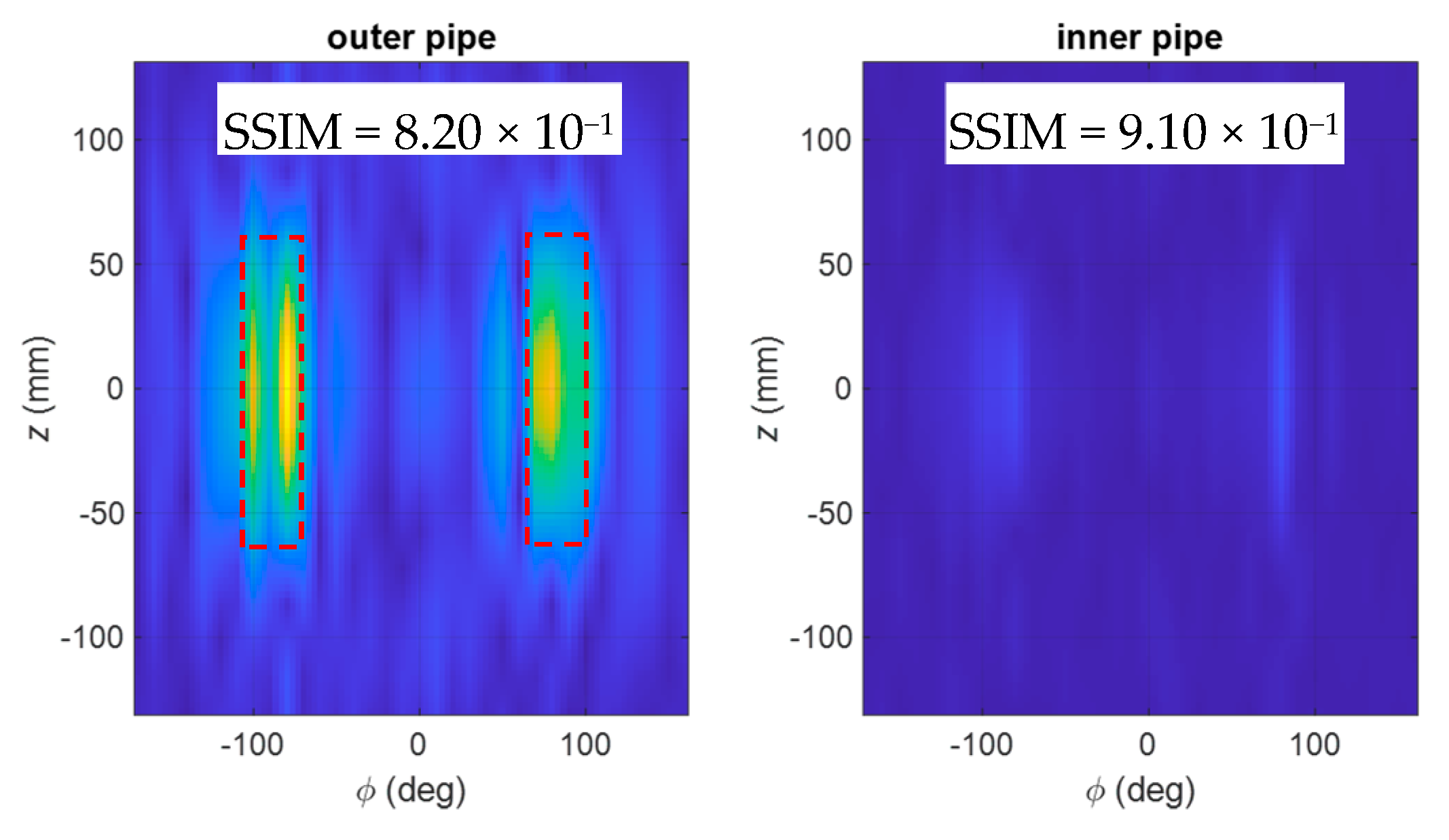
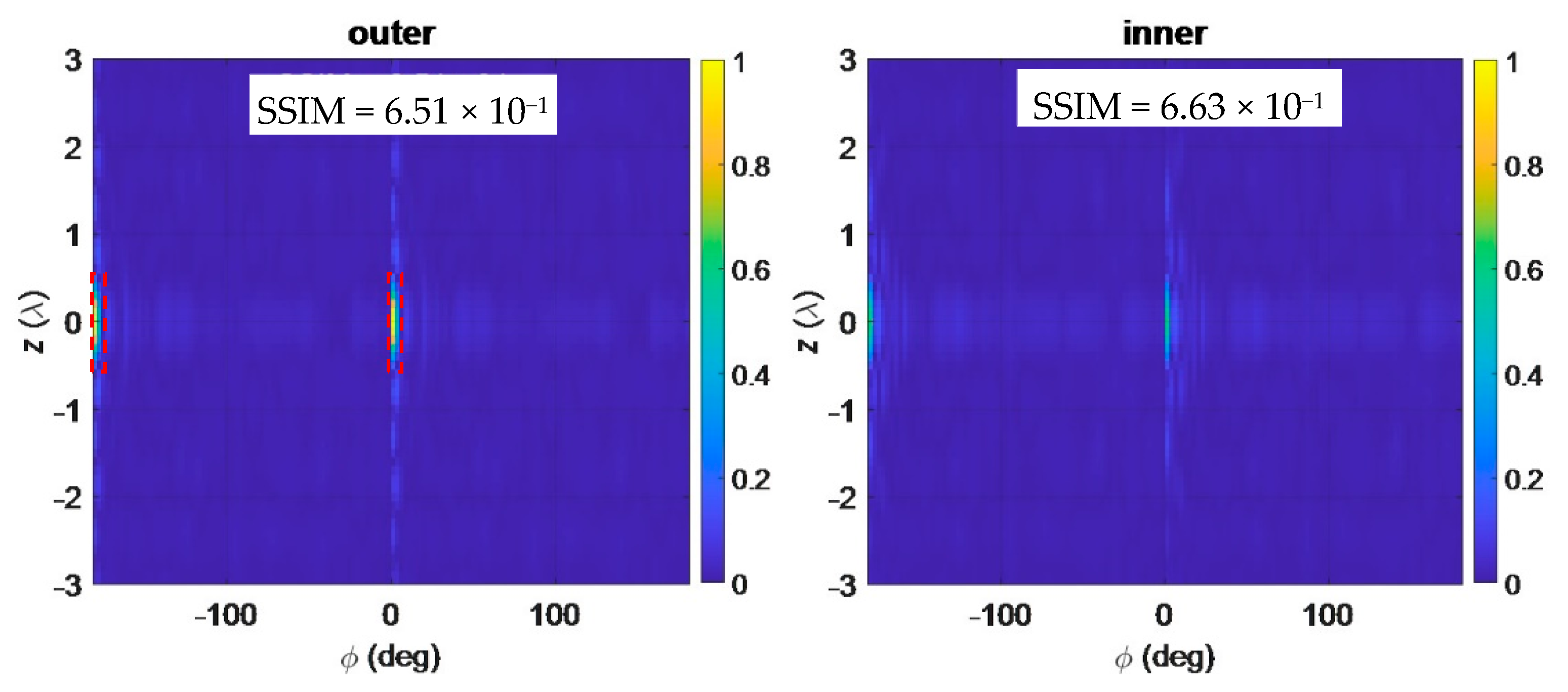
With the responses obtained for PSFs and MGs, implementation of the two-step calibration, applying interpolation, uniform DFT along $\varphi$, DTFT along z, and sLORETA for solving the relevant systems of equations, we reconstruct two sets of 2D images for the two experiments. Figure 12 shows the reconstructed images when the two MGs are placed on the outer pipe with an angular separation of approximately 180$°$. It can be observed that the MGs are detected on the outer pipe with some slight shadows on the image for the inner pipe. The SSIMs for the inner and outer pipe images are close, demonstrating good image quality.

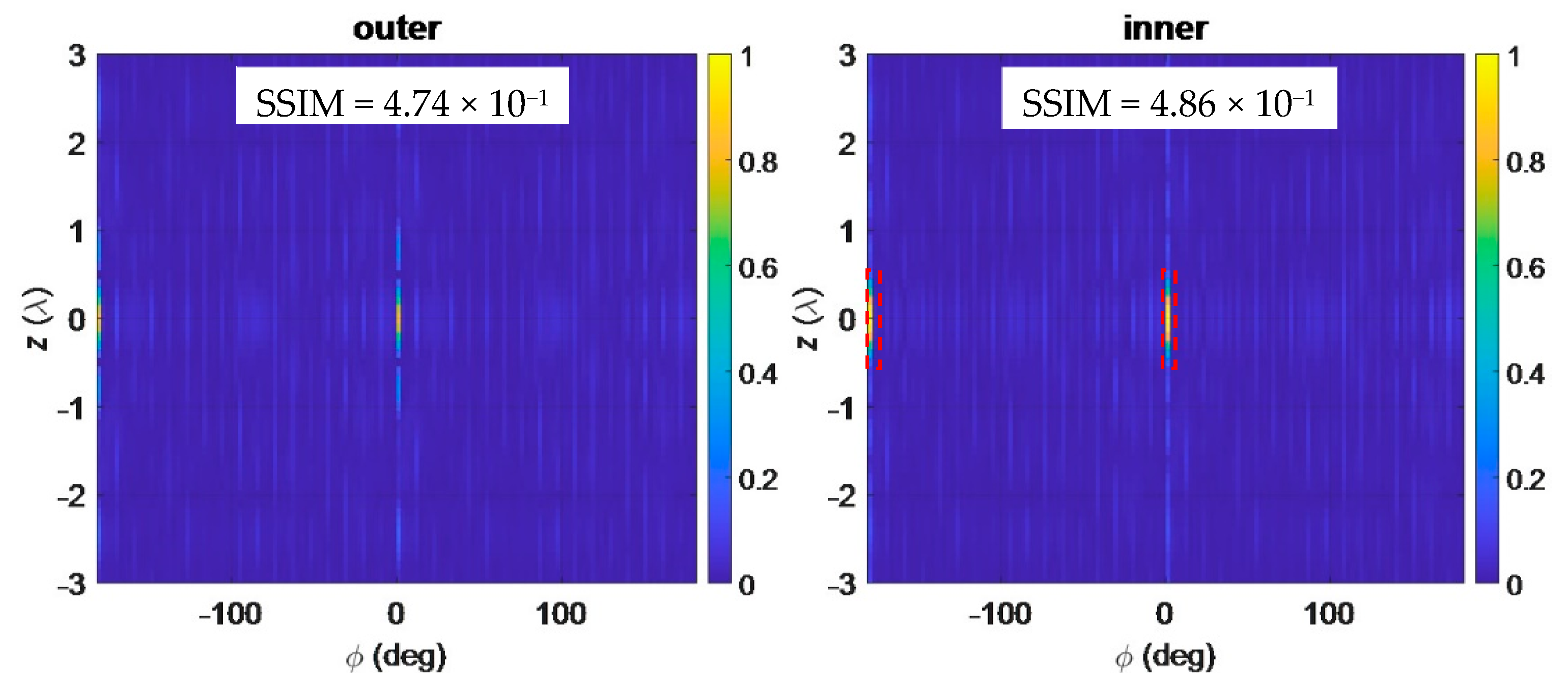
Figure 13 shows the reconstructed images when the two MGs are placed on the inner pipe with an angular separation of approximately 180$°$. From the reconstructed images, it can be observed that the MGs are detected correctly on the inner pipe with some shadows on the outer pipe. The shadows are stronger than those in Figure 12 due to the fact that the responses for the MGs placed on the inner pipe are weaker (the liquid carried by the pipes was very lossy). In Figure 13, the SSIM values for the inner and outer pipe images are close and satisfactory, but, compared to those in Figure 12, the values are lower, as expected.

5. Discussions and Conclusions

In this paper, for the first time, the use of holographic near-field microwave imaging technique with arrays of transmitter and receiver antennas was proposed for the inspection of multiple non-metallic pipes. We utilized a low-cost data acquisition system with arrays of antennas along the azimuthal direction and scanning them along the longitudinal direction. To solve the relevant systems of equations in near-field holographic imaging, we also implemented interpolation, uniform DFT along $\varphi$ and DTFT along z, and sLORETA approach.

Our approach was based on using the Born approximation, which assumes a linear imaging system [21]. This allowed for fast and robust qualitative imaging, which has been already successful in various applications such as airport security scanners [19]. It is worth noting that inspecting longitudinally long structures such as pipelines is not practical using quantitative (non-linear) imaging techniques. This is due to the fact that these optimization-based techniques have long processing times due to iterative solution of an expensive forward model [31].

From our parametric study, it was observed that the images’ quality was better for larger defect sizes. Besides, when reducing the number of frequency data to only one frequency or changing the standoff distance of the antennas by 2 mm, the quality of the reconstructed images degraded compared to the reference case. When changing the property for the inner pipe’s liquid and outer pipe’s liquid by 18% of their true value, the image quality also degraded. Furthermore, for the outer pipe’s liquid property change, the degradation was much more drastic, to the extent that we could not detect the defects anymore.

We also used simulation data to construct 2D images for each pipe for two scenarios: two defects on the inner pipe and two defects on the outer pipe. It was observed that, for both scenarios, the defects were clearly distinguished. When defects were on the outer pipe, the image quality was slightly better, as expected.

In our experimental study, we imaged MGs on two PVC pipes carrying a liquid mixture of water (60%) and glycerin (40%), which is significantly lossy. We tested two scenarios: MGs on the outer pipe and MGs on the inner pipe. From our results, we observed that, in the two studied cases, the MGs were detected. However, it was concluded that the reconstructed images were better when the MGs were on the outer pipe, due to stronger measured responses.

Additionally, the imaging outcome for the non-metallic pipes carrying liquid are affected by temperature. As temperature changes, the dielectric properties for the liquid also changes. For instance, the change of dielectric properties for water with respect to temperature in the microwave regime was reported in [32]. There, for water with a 30 °C temperature change, the dielectric constant changes by approximately 14% at 1 GHz. This amount of change is similar to the uncertainties in the dielectric properties of the liquids studied in our simulation result, where we had a property change of 18%. Obviously, with a higher temperature change, there will be larger image quality deterioration.

In addition, there is a limitation when detecting smaller defects due to the dynamic range of the proposed system. For a common VNA, the dynamic range at frequencies at 1 GHz to 2 GHz is around 100 dB, but for the receiver used in our study, the dynamic range is 63.5 dB. In our preliminary experimental study, we observed that the MGs used in this study were the smallest size that can be imaged reliably. In other words, the dynamic range of the receiver system used in this work limits the sensitivity of detecting smaller MGs/defects.

The proposed system can be used for fast, low-cost, and robust imaging of long, concentric, non-metallic pipes. In this study, PVC pipes were used because they are the most accessible for our proof-of-concept study. However, the proposed imaging system and the results from the parametric study can be extended for different types of non-metallic pipes since most of them have similar dielectric properties (dielectric constant in the range of 2 to 6 with very small loss in the microwave regime). In practice, we envision using such a fast imaging system for inspection of underwater pipeline structures or for above-the-ground pipeline structures. It is important to note that the imaging system for the latter application will be sensitive to the objects and environment around the pipes and proper shielding has to be applied to make the system insensitive to such interferences.

References

- Blitz, J.; Simpson, G. Ultrasonic Methods of Nondestructive Testing; Chapman & Hall: London, UK, 1996. [Google Scholar]
- Alobaidi, W.M.; Alkuam, E.A.; Al-Rizzo, H.M.; Sandgren, E. Applications of ultrasonic techniques in oil and gas pipeline industries: A review. Am. J. Oper. Res. 2015, 5, 4. [Google Scholar] [CrossRef] [Green Version]
- Tong, L.; Mouritz, A.P.; Bannister, M.K. 3D Fiber Reinforced Polymer Composites, 1st ed.; Elsevier Science Ltd.: Oxford, UK, 2002; ISBN 0080439381. [Google Scholar]
- Murphy, K.; Lowe, D. Evaluation of a novel microwave based NDT inspection method for polyethylene joints. In Proceedings of the ASME 2011 Pressure Vessels and Piping Conference, Baltimore, MD, USA, 17–21 July 2011; pp. 321–327. [Google Scholar]
- Zhu, X.W.; Pan, J.P.; Tan, L.J. Microwave scan inspection of HDPE piping thermal fusion welds for lack of fusion defect. Appl. Mech. Mater. 2013, 333–335, 1523–1528. [Google Scholar] [CrossRef]
- Zoughi, R. Microwave Non-Destructive Testing and Evaluation; Kluwer: Dordrecht, The Netherlands, 2000. [Google Scholar]
- Kharkovsky, S.; Zoughi, R. Microwave and millimeter wave nondestructive testing and evaluation–Overview and recent advances. IEEE Instrum. Meas. Mag. 2007, 10, 26–38. [Google Scholar] [CrossRef]
- Case, J.; Shant, K. Microwave NDT: An inspection method. Mater. Eval. 2017, 75, 338–346. [Google Scholar]
- Hinken, J.H. Microwave Testing (μT): An Overview. e-J. Nondestruct. Test. (NDT). Available online: https://www.ndt.net/article/ndtnet/2017/1_Hinken.pdf (accessed on 16 June 2021).
- Stakenborghs, R.J. Microwave inspection method and its application to FRP. In Proceedings of the Materials Technology Institute AmeriTAC Conference, St. Petersburg, FL, USA, 25–28 February 2013; pp. 1–41. [Google Scholar]
- Stakenborghs, R. Microwave based NDE inspection of HDPE pipe welds. In Proceedings of the 17th International Conference on Nuclear Engineering, Brussels, Belgium, 12–16 July 2009; pp. 185–193. [Google Scholar]
- Schmidt, K.; Aljundi, T.; Subaii, G.A.; Little, J. Microwave interference scanning inspection of nonmetallic pipes. In Proceedings of the 5th Middle East Nondestructive Testing Conference & Exhibition, Manama, Bahrain, 9–11 November 2009; pp. 1–15. [Google Scholar]
- Tripathi, D.M.; Gunasekaran, S.; Murugan, S.S.; Enezi, N.A. NDT by microwave test method for non metallic component. In Proceedings of the Indian National Seminar & Exhibition on Non-Destructive Evaluation NDE, Thiruvananthapuram, Indian, December 2016; pp. 115–121. Available online: https://www.ndt.net/article/nde-india2016/papers/A147.pdf (accessed on 16 June 2021).
- Carrigan, T.D.; Forrest, B.E.; Andem, H.N.; Gui, K.; Johnson, L.; Hibbert, J.E.; Lennox, B.; Sloan, R. Nondestructive testing of nonmetallic pipelines using microwave reflectometry on an in-line inspection robot. IEEE Trans. Instrum. Meas. 2019, 68, 586–594. [Google Scholar] [CrossRef] [Green Version]
- Ghasr, M.T.; Ying, K.; Zoughi, R. 3D millimeter wave imaging of vertical cracks and its application for the inspection of HDPE pipes. AIP Conf. Proc. 2014, 1581, 1531–1536. [Google Scholar]
- Laviada, J.; Wu, B.; Ghasr, M.T.; Zoughi, R. Nondestructive evaluation of microwave-penetrable pipes by synthetic aperture imaging enhanced by full-wave field propagation model. IEEE Trans. Instrum. Meas. 2019, 68, 1112–1119. [Google Scholar] [CrossRef]
- Wu, B.; Gao, Y.; Laviada, J.; Ghasr, M.T.; Zoughi, R. Time-reversal SAR imaging for nondestructive testing of circular and cylindrical multi-layered dielectric structures. IEEE Trans. Instrum. Meas. 2020, 69, 2057–2066. [Google Scholar] [CrossRef] [Green Version]
- Buhari, M.D.; Tian, G.Y.; Tiwari, R. Microwave-based SAR technique for pipeline inspection using autofocus range-Doppler algorithm. IEEE Sens. J. 2019, 19, 1777–1787. [Google Scholar] [CrossRef] [Green Version]
- Sheen, D.M.; McMakin, D.L.; Hall, T.E. Three-dimensional millimeter-wave imaging for concealed weapon detection. IEEE Trans. Microw. Theory Tech. 2001, 49, 1581–1592. [Google Scholar] [CrossRef]
- Wu, H.; Ravan, M.; Sharma, R.; Patel, J.; Amineh, R.K. Microwave holographic imaging of nonmetallic concentric pipes. IEEE Trans. Instrum. Meas. 2020, 69, 7594–7605. [Google Scholar] [CrossRef]
- Amineh, R.K.; McCombe, J.; Khalatpour, A.; Nikolova, N.K. Microwave holography using point-spread functions measured with calibration objects. IEEE Trans. Instrum. Meas. 2015, 64, 403–417. [Google Scholar] [CrossRef]
- Sheen, D.M.; McMakin, D.; Hall, T.E. Near-field three-dimensional radar imaging techniques and applications. Appl. Opt. 2010, 49, E83–E93. [Google Scholar] [CrossRef]
- Wu, H.; Ravan, M.; Amineh, R.K. Holographic near-field microwave imaging with antenna arrays in a cylindrical setup. IEEE Trans. Microw. Theory Tech. 2021, 69, 418–430. [Google Scholar] [CrossRef]
- Wu, H.; Amineh, R.K. A low-cost and compact three-dimensional microwave holographic imaging system. Electronics 2019, 8, 1036. [Google Scholar] [CrossRef] [Green Version]
- Sheen, D.M.; McMakin, D.L.; Hall, T.E. Cylindrical millimeter-wave imaging technique for concealed weapon detection. Proc. SPIE Int. Soc. Opt. Eng. 1998, 3240, 242–250. [Google Scholar]
- Capozzoli, A.; Curcio, C.; Liseno, A. Singular value optimization in inverse electromagnetic scattering. IEEE Antennas Wirel. Propag. Lett. 2017, 16, 1094–1097. [Google Scholar] [CrossRef]
- Martin, L.E.; Fouda, A.E.; Amineh, R.K.; Capoglu, I.; Donderici, B.; Roy, S.S.; Hill, F. New high-definition frequency tool for tubing and multiple casing corrosion detection. In Proceedings of the Abu Dhabi International Petroleum Exhibition & Conference, Abu Dhabi, United Arab Emirates, 13–16 November 2017; pp. 1–14. [Google Scholar]
- Renardy, Y.; Joseph, D.D. Couette flow of two fluids between concentric pipes. J. Fluid Mech. 1985, 150, 381–384. [Google Scholar] [CrossRef] [Green Version]
- Wang, Z.; Bovik, A.C.; Sheikh, H.R.; Simoncelli, E.P. Image quality assessment: From error visibility to structural similarity. IEEE Trans. Image Process. 2004, 13, 600–612. [Google Scholar] [CrossRef] [Green Version]
- Meaney, P.M.; Fox, C.J.; Geimer, S.D.; Paulsen, K.D. Electrical characterization of glycerin: Water mixtures: Implications for use as a coupling medium in microwave tomography. IEEE Trans. Microw. Theory Tech. 2017, 65, 1471–1478. [Google Scholar] [CrossRef]
- Zaeytijd, J.D.; Franchois, A.; Eyraud, C.; Geffrin, J. Full-wave three-dimensional microwave imaging with a regularized Gauss–Newton method—Theory and experiment. IEEE Trans. Antennas Propag. 2007, 55, 3279–3292. [Google Scholar] [CrossRef]
- Vijay, R.; Jain, R.; Sharma, K.S. Dielectric properties of water at microwave frequencies. Int. J. Eng. Res. Tech. 2014, 3, 1–3. [Google Scholar]
Figure 1.
(a) Illustration of the imaging setup and (b) top view of the setup.
Figure 2.
Illustration of the simulation setup in FEKO.
Figure 3.
Reconstructed images of the reference case (RI: reconstructed image and TI: true image).
Figure 4.
Reconstructed images of the larger defects (RI: reconstructed image and TI: true image).
Figure 5.
Reconstructed images of the reference case using single frequency data (RI: reconstructed image and TI: true image).
Figure 6.
Reconstructed images with an added standoff distance of 2 mm (RI: reconstructed image and TI: true image).
Figure 7.
Reconstructed images when the property of the inner pipe’s liquid is not correct for PSFs (RI: reconstructed image and TI: true image).
Figure 8.
The reconstructed images when the property of the outer pipe’s liquid is not correct for PSFs (RI: reconstructed image and TI: true image).
Figure 9.
Reconstructed 2D images for two defects on the inner pipe. The red, dashed lines show the locations of the defects.
Figure 10.
Reconstructed 2D images for two defects on the outer pipe. The red, dashed lines show the locations of the defects.
Figure 11.
(a) Picture of the main components for the imaging system and (b) data acquisition circuitry.
Figure 12.
Reconstructed 2D images with MGs placed on the outer pipe. The red, dashed lines show the locations of the MGs.
Figure 13.
Reconstructed 2D images with MGs placed on the inner pipe. The red, dashed lines show the locations of the MGs.
Publisher’s Note: MDPI stays neutral with regard to jurisdictional claims in published maps and institutional affiliations. |
© 2021 by the authors. Licensee MDPI, Basel, Switzerland. This article is an open access article distributed under the terms and conditions of the Creative Commons Attribution (CC BY) license (https://creativecommons.org/licenses/by/4.0/).
Share and Cite
MDPI and ACS Style
Gao, Y.; Ravan, M.; K. Amineh, R. Fast, Robust, and Low-Cost Microwave Imaging of Multiple Non-Metallic Pipes. Electronics 2021, 10, 1762. https://0-doi-org.brum.beds.ac.uk/10.3390/electronics10151762
AMA Style
Gao Y, Ravan M, K. Amineh R. Fast, Robust, and Low-Cost Microwave Imaging of Multiple Non-Metallic Pipes. Electronics. 2021; 10(15):1762. https://0-doi-org.brum.beds.ac.uk/10.3390/electronics10151762
Chicago/Turabian StyleGao, Yuki, Maryam Ravan, and Reza K. Amineh. 2021. "Fast, Robust, and Low-Cost Microwave Imaging of Multiple Non-Metallic Pipes" Electronics 10, no. 15: 1762. https://0-doi-org.brum.beds.ac.uk/10.3390/electronics10151762
Note that from the first issue of 2016, this journal uses article numbers instead of page numbers. See further details here.