Performance Evaluation of Offline Speech Recognition on Edge Devices

Abstract

Deep learning–based speech recognition applications have made great strides in the past decade. Deep learning–based systems have evolved to achieve higher accuracy while using simpler end-to-end architectures, compared to their predecessor hybrid architectures. Most of these state-of-the-art systems run on backend servers with large amounts of memory and CPU/GPU resources. The major disadvantage of server-based speech recognition is the lack of privacy and security for user speech data. Additionally, because of network dependency, this server-based architecture cannot always be reliable, performant and available. Nevertheless, offline speech recognition on client devices overcomes these issues. However, resource constraints on smaller edge devices may pose challenges for achieving state-of-the-art speech recognition results. In this paper, we evaluate the performance and efficiency of transformer-based speech recognition systems on edge devices. We evaluate inference performance on two popular edge devices, Raspberry Pi and Nvidia Jetson Nano, running on CPU and GPU, respectively. We conclude that with PyTorch mobile optimization and quantization, the models can achieve real-time inference on the Raspberry Pi CPU with a small degradation to word error rate. On the Jetson Nano GPU, the inference latency is three to five times better, compared to Raspberry Pi. The word error rate on the edge is still higher, but it is not too far behind, compared to that on the server inference.

1. Introduction

Automatic speech recognition (ASR) is a process of converting speech signals to text. It has a large number of real-world use cases, such as dictation, accessibility, voice assistants, AR/VR applications, captioning of videos, podcasts, searching audio recordings, and automated answering services, to name a few. On-device ASR makes more sense for many use cases where an internet connection is not available or cannot be used. Private and always-available on-device speech recognition can unblock many such applications in healthcare, automotive, legal and military fields, such as taking patient diagnosis notes, in-car voice command to initiate phone calls, real-time speech writing, etc.

Deep learning–based speech recognition has made great strides in the past decade [1]. It is a subfield of machine learning which essentially mimics the neural network structure of the human brain for pattern matching and classification. It typically consists of an input layer, an output layer and one or more hidden layers. The learning algorithm adjusts the weights between different layers, using gradient descent and backpropagation until the required accuracy is met [1,2]. The major reason for its popularity is that it does not need feature engineering. It autonomously extracts the features based on the patterns in the training dataset. The dramatic progress of deep learning in the past decade can be attributed to three main factors [3]: (1) large amounts of transcribed data sets; (2) rapid increase in GPU processing power; and (3) improvements in machine learning algorithms and architectures. Computer vision, object detection, speech recognition and other similar fields have advanced rapidly because of the progress of deep learning.

The majority of speech recognition systems run in backend servers. Since audio data need to be sent to the server for transcription, the privacy and security of the speech cannot be guaranteed. Additionally, because of the reliance on a network connection, the server-based ASR solution cannot always be reliable, fast and available.

On the other hand, on-device-based speech recognition inherently provides privacy and security for the user speech data. It is always available and improves the reliability and latency of the speech recognition by precluding the need for network connectivity [4]. Other non-obvious benefits of edge inference are energy and battery conservation for on-the-go products by avoiding Bluetooth/Wi-Fi/LTE connection establishments for data transfers.

Inferencing on edge can be achieved either by running computations on CPU or on hardware accelerators, such as GPU, DSP or using dedicated neural processing engines. The benefits and demand for on-device ML is driving modern phones to have dedicated neural engine or tensor processing units. For example, Apple iOS 15 will support on-device speech recognition for iPhones with Apple neural engine [5]. The Google Pixel 6 phone comes equipped with a tensor processing unit to handle on-device ML, including speech recognition [6]. Though dedicated neural hardwares might become a general trend in the future, at least in the short term, a large majority of IoT, mobile or wearable devices will not have these dedicated hardwares for on-device ML. Hence, training the models on backend and then pre-optimizing for CPU or general purpose GPU-based edge inferencing is a practical near term solution for on-edge inference [4].

In this paper, we evaluate the performance of ASR on Raspberry Pi and Nvidia Jetson Nano. Since the CPU, GPU and memory specification of these two devices are similar to those of typical edge devices, such as smart speakers, smart displays, etc., the evaluation outcomes in this paper should be similar to the results on a typical edge device. Related to our work, large vocabulary continuous speech recognition was previously evaluated on an embedded device, using CMU SPHINX-II [7]. In [8], the authors evaluated the on-device speech recognition performance with DeepSpeech [9], Kaldi [10] and Wav2Letter [11] models. Moreover, most on-the-edge evaluation papers focus on computer vision tasks, using CNN [12,13]. To the best of our knowledge, there have been no evaluations done for any type of transformer-based speech recognition models on low power edge devices, using both CPU- and GPU-based inferencing. The major contributions of this paper are as follows:

• We present the steps for preparing and inferencing the pre-trained PyTorch models for on edge CPU- and GPU-based inferencing.
• We measure and analyze the accuracy, latency and computational efficiency of ASR inference with transformer-based models on Raspberry Pi and Jetson Nano.
• We also provide a comparative analysis of inference between CPU- and GPU-based processing on edge.

The rest of the paper is organized as follows: In the background section, we discuss ASR and transformers. In the experimental setup, we go through the steps for preparing the models and setting up both the devices for inferencing. We highlight some of the challenges we faced while setting up the devices. We go over the accuracy, performance and efficiency metrics in the results section. Finally, we conclude with the summary and outlook.

2. Background

ASR is the process of converting audio signals to text. In simple terms, the audio signal is divided into frames and passed through fast Fourier transform to generate feature vectors. This goes through an acoustic model to output the probability distribution of phonemes. Then, a decoder with a lexicon, vocabulary and language model is used to generate the word n-grams distributions. The hidden Markov model (HMM) [14] with a Gaussian mixture model (GMM) [15] was considered a mainstream ASR algorithm until a decade ago. Conventionally, the featurizer, acoustic modeling, pronunciation modeling, and decoding all were built separately and composed together to create an ASR system. Hybrid HMM–DNN approaches replaced GMM with deep neural networks with significant performance gains [16]. Further advances used CNN- [17,18] and RNN-based [19] models to replace some or all components in hybrid DNN [1,2] architecture. Over time, ASR model architectures have evolved to convert audio signals to text directly, called sequence-to-sequence models. These architectures have simplified the training and implementation of ASR models.The most successful end-to-end ASR are based on connectionist temporal classification (CTC) [20], recurrent neural network (RNN) transducer (RNN-T) [19], and attention-based encoder–decoder architecture [21].

Transformer is a sequence-to-sequence architecture originally proposed for machine translation [22]. When used for ASR, the input of transformer is audio frames instead of the text input, as in translation use case. Transformer uses multi head attention and positional embeddings. It learns sequential information through a self-attention mechanism instead of the recurrent connection used in RNN. Since their introduction, transformers are increasingly becoming the model of choice for NLP problems. The powerful natural language processing (NLP) models, such as GPT-3 [23], BERT [24], and AlphaFold 2 [25], which is the model that predicts the structures of proteins from their genetic sequences, are all based on transformer architecture. The major advantages of transformers over RNN/LSTM [26] is that they process the whole sequence at once, enabling parallel computation and hence, reducing the training time. They also do not suffer from long dependency issues; hence, they are more accurate. Since the transformer processes the whole sequence at once, they are not directly suitable for streaming-based applications, such as continuous dictation. In addition, their decoding complexity is quadratic over input sequence length because the attention is computed pairwise for each input. In this paper, we focus on the general viability and computational cost of transformer-based ASR on audio files. In future, we plan to explore streaming supported transformer architectures on edge.

2.1. Wav2Vec 2.0 Model

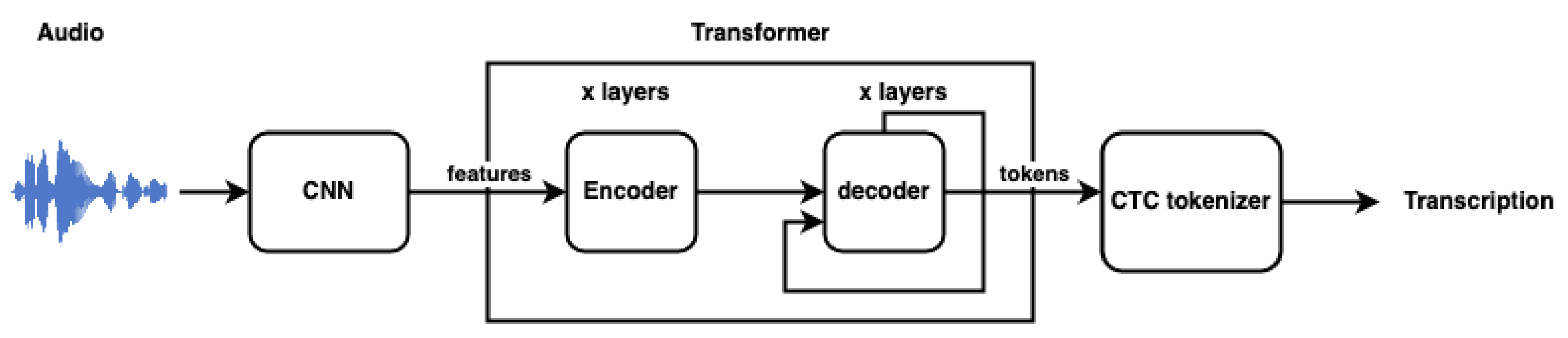
Wav2Vec 2.0 is a transformer-based speech recognition model trained using a self-supervised method with contrastive training [27]. The raw audio is encoded using a multilayer convolutional network, the output of which is fed to the transformer network to build latent speech representations. Some of the input representations are masked during training. The model is then fine tuned with a small set of labeled data, using the connectionist temporal classification (CTC) [20] loss function. The great advantage of Wav2Vec 2.0 is the ability to learn from unlabeled data, which is tremendously useful in training for speech recognition for languages with very limited labeled audio. For the remaining part of this paper, we refer to the Wav2Vec 2.0 model as Wav2Vec to reduce verbosity. In our evaluation, we use a pre-trained base Wav2Vec model, which was trained on 960 hr of unlabeled LibriSpeech audio. We evaluate a 100 hr and a 960 hr fine-tuned model.

Figure 1 shows the simplified flow of the ASR process with this model.

2.2. Speech2Text Model

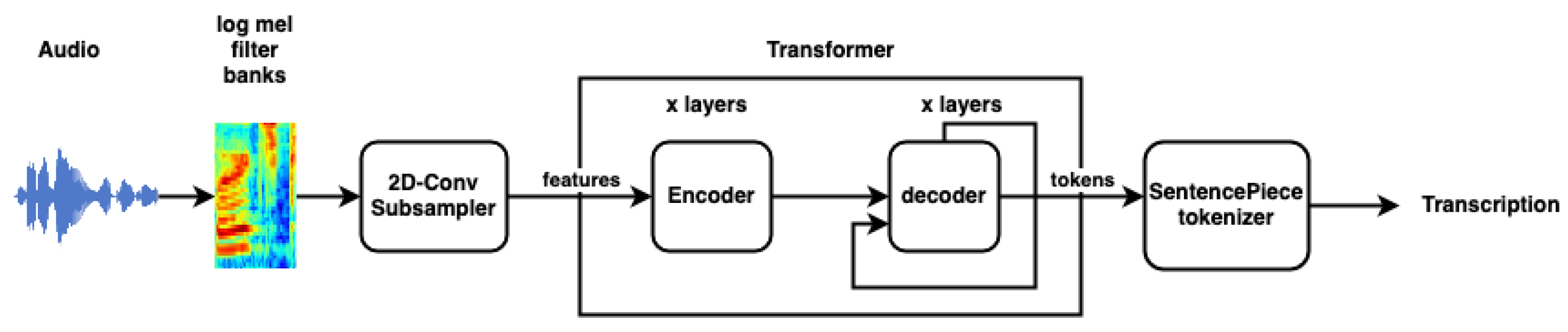
The Speech2Text model is a transformer-based speech recognition model trained using the supervised method [28]. The transformer architecture is based on [22]. In addition, it has an input subsampler. The purpose of the subsampler is to downsample the audio sequence to match the input dimensions of the transformer encoder. The model is trained with a LibriSpeech, 960 hr, labeled training data set. Unlike Wav2Vec, which takes raw audio samples as input, this model accepts 80-channel log Mel filter bank extracted features with a 25 ms window size and 10 ms shift. Additionally, utterance-level cepstral mean and variance normalization (CMVN) [29] is applied on the input frames before feeding to the subsampler. The decoder uses a 10,000 unigram vocabulary.

Figure 2 shows the simplified flow of the ASR process with this model.

3. Experimental Setup

3.1. Model Preparation

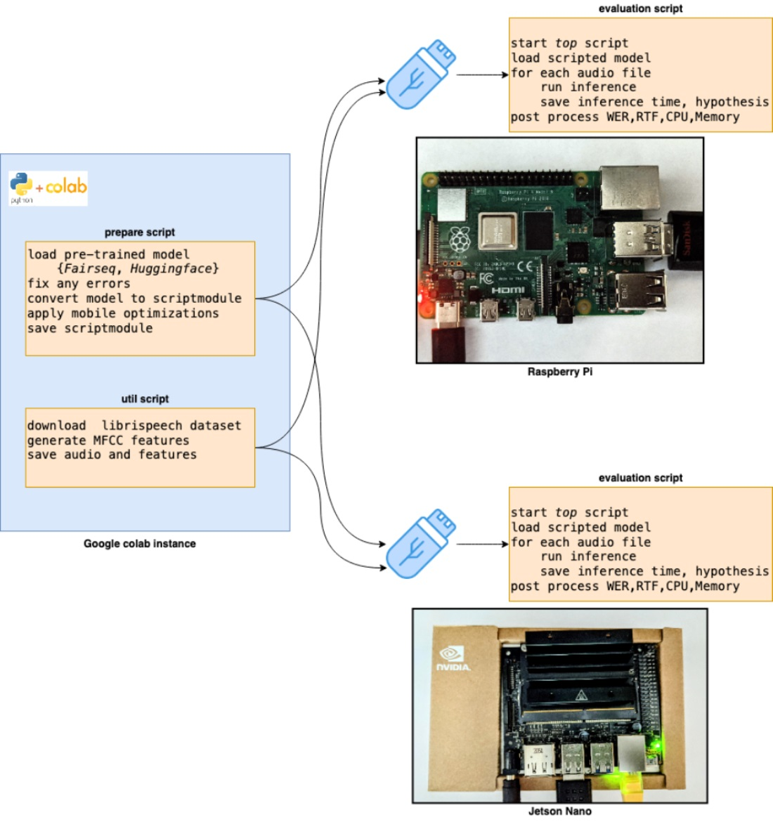
We use PyTorch models for evaluation. PyTorch is an open-source machine learning framework based on the Torch library. Figure 3 shows the steps for preparing the models for inferencing on edge devices.

We first go through a few of the PyTorch tools and APIs used in our evaluation.

3.1.1. TorchScript

TorchScript is the means by which PyTorch models can be optimized, serialized and saved in intermediate representation (IR) format. torch.jit (https://pytorch.org/docs/stable/jit.html (accessed on 30 October 2021)) APIs are used for converting, saving and loading PyTorch models as ScriptModules. TorchScript itself is a subset of the Python language. As a result, sometimes, a model written in Python needs to be simplified to convert it into a script module. The TorchScript module can be created either using tracing or scripting methods. Tracing works by executing the model with sample inputs and capturing all computations, whereas scripting performs static inspection to go through the model recursively. The advantage of scripting over tracing is that it correctly handles the loops and control statements in the module. A saved script module can then be loaded either in a Python or C++ environment for inferencing purposes. For our evaluation, we generated ScriptModules for both Speech2Text and Wav2Vec models after applying any valid optimizations for specific devices.

3.1.2. PyTorch Mobile Optimizations

PyTorch provides a set of APIs for optimizing the models for mobile platforms. It uses module fusing, operator fusing, and quantization among other things to optimize the models. We apply dynamic quantization for models used in this experiment. During this quantization, the scale factors are determined for activations dynamically based on the data range observed at runtime. By quantization, a neural network is converted to use a reduced precision integer representation for the weights and/or activations. This saves on model size and allows the use of higher throughput math operations on CPU or GPU.

3.1.3. Models

We evaluated the Speech2Text and Wav2Vec transformer-based models on Raspberry Pi and Nvidia Jetson Nano. Inference on Raspberry Pi happens on CPU, while on Jetson Nano, it happens on GPU, using CUDA APIs. Given the limited RAM, CPU, and storage on these devices, we make use of Google Colab for importing, optimizing and saving the model as a TorchScript module. The saved modules are copied to Raspberry Pi and Jetson Nano for inferencing. On Raspberry Pi, which uses CPU-based inference, we evaluate both quantized and unquantized models. On Jetson Nano, we only evaluate unquantized models since CUDA only supports floating point operations.

Speech2Text Model

The Speech2Text pre-trained model is imported from fairseq (https://github.com/pytorch/fairseq/tree/master/examples/speech_to_text (accessed on 30 October 2021)). Fairseq is a sequence modeling toolkit that allows researchers and developers to train custom models for speech and text tasks. We needed to make minor syntactical changes, such as Python type hints, to export the generator model as a TorchScript module. We have used s2t_transformer_s small architecture for this evaluation. The decoding uses a beam search decoder with a beam size of 5 and a SentencePiece tokenizer.

Wav2Vec Model

Wav2Vec pre-trained models are imported from huggingface (https://huggingface.co/transformers/model_doc/wav2vec2.html (accessed on 30 October 2021)) using the Wav2Vec2ForCTC interface. We have used Wav2Vec2CTCTokenizer to decode the output indexes into transcribed text.

3.2. Raspberry Pi Setup

Raspberry Pi 4 B is used in this evaluation. The device specs are provided in

Table 1. Raspberry Pi 4 B specs.

Name	Spec
Chip	BCM2711
CPU	Quad core Cortex-A72 (ARM v8) 64-bit SoC
Clock speed	1.5 GHz
RAM	4 GB SDRAM
Caches	32 KB data + 48 KB instruction L1 cache per core. 1 MB L2 cache
Storage	32 GB micro SD card
OS	64 bit Raspberry Pi OS
Python version	3.7
Power supply	5 V DC via USB-C connector

. The default Raspberry Pi OS is 32 bit, which is not compatible with PyTorch. Hence, we installed a 64 bit OS.

The main Python package required for inferencing is PyTorch. The default prebuilt wheel files of this package are mainly for Intel architecture, which depend on Intel-MKL (math kernel library) for math routines on CPU. The ARM-based architectures cannot use Intel MKL. They instead have to use QNNPACK/XNNPACK backend with other BLAS (basic linear algebra subprograms) libraries. QNNPACK (https://github.com/pytorch/QNNPACK (accessed on 30 October 2021)) (quantized neural networks package) is a mobile-optimized library for low-precision, high-performance neural network inference. Similarly, XNNPACK (https://github.com/google/XNNPACK (accessed on 30 October 2021)) is a mobile-optimized library for higher precision neural network inference. We built and installed the torch wheel file on Raspberry Pi from source with XNNPACK and QNNPACK cmake configs. We needed to set the device backend to QNNPACK during inference as torch.backends.quantized.engine=’qnnpack’. Note that with the latest PyTorch release 1.9.0, the wheel files are available for ARM 64-bit architectures. Hence, there is no need to build torch from source anymore.

The lessons learnt during setup are as follows:

• Speech2Text transformer models expect Mel-frequency cepstral coefficients [30] as input features. However, we could not use Torchaudio, PyKaldi, librosa or python_speech_features libraries for this because of dependency issues. Torchaudio has dependency on Intel MKL. Building PyKaldi on device was not feasible because of memory limitations. The librosa and python_speech_features packages produced different outputs for MFCC, which were unsuitable for PyTorch models. Therefore, the MFCC features for the LibriSpeech data set were pre-generated, using fairseq audio_utils (https://github.com/pytorch/fairseq/blob/master/fairseq/data/audio/audio_utils.py (accessed on 30 October 2021)) on the server, and saved as NumPy files. These NumPy files were used as model input after applying CWVN transforms.
• Running pip install with or without sudo while installing packages, can cause silent dependency issues. This is especially true when the same package is installed multiple times with and without using sudo.
• To experiment with huggingface transformer models, the datasets package is required, which in turn has dependency on PyArrow (an Apache arrow library). Arrow library needs to be built and installed from source to use PyArrow.

3.3. Nvidia Jetson Nano Setup

We configured Jetson Nano using the instructions on the Nvidia website. The Nano flash file comes with JetPack pre-installed, which includes all the CUDA libraries required for inferencing on GPU. The full specs of the device are provided in

Table 2. Jetson Nano specs.

Name	Spec
GPU	128-core Maxwell
CPU	Quad-core ARM A57
Clock speed	1.43 GHz
Memory	4 GB 64-bit LPDDR4
Caches	262,144 bytes L2 cache
Storage	32 GB micro SD card
OS	Ubuntu 18.04.5 LTS
Python version	3.6
CUDA	10.2
nvidia-jetpack	4.5.1-b17
Power supply	Barrel jack 5 V 4 A

.

For Nano, we needed to build torch from source with CUDA cmake option. Further, an upgrade was needed to Clang and LLVM compiler toolchain to use Clang for compiling PyTorch.

The lessons learnt during setup are as follows:

• Need to use 5 V, 4 A barrel jack power supply for Jetson Nano. The USB C power supply does not provide sufficient power for continuous speech-to-text inferencing on CUDA.
• cuDNN benchmarking needs to be switched on for Nano to pick up the speed while executing. It takes a very long time for Nanto to execute the initial few samples. That is because the cuDNN tries to find the best algorithm for the configured input. After that, the RTF improves significantly and it executes very quickly.
• Jetson Nano froze on long duration audios while inferencing with the Wav2Vec model. Through trial and error, we figured out that by limiting the input audio duration to 8 s and batching the inputs to be of size 64 K (4 s audio) or less, we can allow the inference to continue without hiccups.

3.4. Evaluation Methodology

This section explains the methodologies used for collecting and presenting the metrics in this paper. The LibriSpeech [31] test and dev datasets were used to evaluate ASR performance on both Raspberry Pi and Jetson Nano. The test and dev datasets together contain 21 hr of audio. To save time, for these experiments we randomly sampled 300 (∼10%) of the audio files in each of the four data sets for inference. The same set for each configuration was used so that the results would be comparable. Typically, ML practitioners only report the WER metric for server-based ASR. So, we did not have a server side reference for latency and efficiency metrics, such as memory, CPU or load times. Unlike backend servers, the edge devices are constrained in terms of memory, CPU, disk and energy. To achieve on-device ML, the inferencing needs to be efficient enough to fit within the device’s resource budgets. Hence, we measured these efficiency metrics along with the accuracy to assess the plausibility of meeting these budgets on typical edge devices.

3.4.1. Accuracy

Accuracy is measured using word error rate (WER), a standard metric for speech-to-text tasks. It is defined as in Equation (1):

$$WER=(S+I+D)/N$$

(1)

where S is the number of substitutions, D is the number of deletions, I is the number of insertions and N is the number of words in the reference.

WER for a dataset is computed as the total number of errors over the total number of reference words in the dataset. We compare the on-device WER on Raspberry Pi and Jetson Nano with the on-server-based WER as reported in Speech2Text [28] and Wav2Vec [27] papers. In both papers, the WER for all models was computed on LibriSpeech test and dev data sets with GPU in standalone mode. On server, the Speech2Text model used a beam size of 5 and vocabulary of 10,000 words for decoding, whereas the Wav2Vec model used a transformer-based language model for decoding. The pre-trained models used in this experiment have the same configuration as that of the server models.

3.4.2. Latency

The latency of ASR is measured using real time factor (RTF). It is defined in Equation (2). In simple terms, with a RTF of 0.5, two seconds of audio will be transcribed by the system in one second.

$$RTF=(readtime+inferencetime+decodingtime)/totaluttteranceduration$$

(2)

We compute the avg, mean, pctl 75 and pctl 90 RTF over all the audio samples in each data set. We also used PyTorch profiler to visualize the CPU usage of various operators and functions inside the models.

3.4.3. Efficiency

We measure the CPU load and memory footprint during the entire data set evaluation, using the Linux top command. The top command is executed in the background every two minutes in order to avoid side effects on the main inference script.

The model load time is measured by collecting the torch.jit.load API latency to load the scripted model. We separately measured the load time by running 10 iterations and took an average. We ensured that the load time measurements were from a clean state, i.e., from the system boot, to discount any caching in the Linux OS layer for subsequent model loads.

4. Results

In this section, we present the accuracy, performance and efficiency metrics for Speech2Text and Wav2Vec model inference.

4.1. WER

Table 3. WER on Raspberry Pi.

Test Dataset				Dev Dataset
Dataset	Model	Edge WER	Server WER	Dataset	Model	Edge WER	Server WER
test-clean	S2T_q	4.7%		dev-clean	S2T_q	4.3%
	S2T	4.4%	4.4%		S2T	3.9%	3.8%
	W2V100q	7.3%			W2V100q	7.9%
	W2V100	6.9%	2.6%		W2V100	7.8%	2.2%
	W2V960q	4.1%			W2V960q	4.3%
	W2V960	4.1%	2.1%		W2V960	3.6%	1.8%
test-other	S2T_q	11.7%		dev-other	S2T_q	11.1%
	S2T	11.0%	9.0%		S2T	10.6%	8.9%
	W2V100q	16.2%			W2V100q	15.1%
	W2V100	15.6%	6.3%		W2V100	14.9%	6.3%
	W2V960q	10.8%			W2V960q	10.2%
	W2V960	9.7%	4.8%		W2V960	9.8%	4.7%

and

Table 4. WER on Jetson Nano.

Test Dataset				Dev Dataset
Dataset	Model	Edge WER	Server WER	Dataset	Model	Edge WER	Server WER
test-clean	S2T	4.4%	4.4%	dev-clean	S2T	3.3%	3.8%
	W2V100	9.5%	2.6%		W2V100	10.2%	2.2%
	W2V960	6.4%	2.1%		W2V960	6.2%	1.8%
test-other	S2T	8.6%	9.0%	dev-other	S2T	9.8%	8.9%
	W2V100	20.5%	6.3%		W2V100	19.7%	6.3%
	W2V960	13.1%	4.8%		W2V960	13.0%	4.7%

show the WER on Raspberry Pi and Jetson Nano, respectively.

The WER is slightly higher for the quantized models, compared to the unquantized ones by an avg of ∼0.5%. This is a small trade off in accuracy for better RTF and efficient inference. The test-other and dev-other data sets have a higher WER, compared to the test-clean and dev-clean data sets. This is expected because other datasets are noisier, compared to clean ones.

The WER on device for unquantized models is generally higher than what is reported on the server. We need to investigate further to understand this discrepancy. One plausible reason could be due to a smaller sampled dataset used in our evaluation, compared to the server WER, which is calculated over the entire dataset.

WER for the Wav2Vec case is higher because of batching of the input samples at the 64 K (4 s audio) boundary. If a sample duration is longer than 4 s, we divide it into two batches. See Section 3.3 for the reasoning. So, words at the boundary of 4 s can be misinterpreted. We plan to investigate this batching problem in future. We report the WER figures here for the purpose of completeness.

4.2. RTF

In our experiments, RTF is dominated by model inference time > 99% compared to other two factors in (2).

Table 5. RTF of Raspberry Pi.

Model	Avg	Mean	P75	P90
Speech2Text	0.33	0.33	0.38	0.45
Speech2Text quantized	0.29	0.29	0.34	0.39
Wav2Vec 100 hr	1.43	1.42	1.45	1.5
Wav2Vec 100 hr quantized	1.00	0.97	1.03	1.11
Wav2Vec 960 hr	1.49	1.48	1.54	1.58
Wav2Vec 960 hr quantized	1.03	1.00	1.07	1.18

and

Table 6. RTF on Jetson Nano.

Model	Avg	Mean	P75	P90
Speech2Text	0.13	0.13	0.15	0.17
Wav2Vec 100 hr	0.22	0.22	0.25	0.28
Wav2Vec 960 hr	0.23	0.22	0.26	0.29

show the RTF for Raspberry Pi and Jetson Nano, respectively. RTF does not vary between different data sets for the same models. Hence, we show the RTF (avg, mean, pctl 75 and pctl 90) per model instead of one per data set.

RTF is improved by ∼10% for quantized models, compared to unquantized floating point models. This is because CPU has to load less memory and can run tensor computations more efficiently in int8 than in floating points. The inferencing of the Speech2Text model is three times faster than the Wav2Vec model. This can be explained by the fact that the Wav2Vec has three times more parameters than the Speech2Text model (refer to

Table 7. Model size.

Model Name	Size	Parameters
Speech2Text quantized	80 MB	30 Million
Speech2Text	125 MB
Wav2Vec quantized	207 MB	93 Million
Wav2Vec	377 MB

). There is no noticeable difference in RTF between 100 hr and 960 hr fine-tuned Wav2Vec models because the number of parameters do not change between 960 hr and 100 hr fine-tuned models.

RTF on Jetson Nano is three times better for the Speech2Text model and five times better for the Wav2Vec model, compared to Raspberry Pi. Nano is able to make use of a large number of CUDA cores for tensor computations. We do not evaluate quantized models on Nano because CUDA only supports floating point computations.

Wav2Vec RTF on Raspberry Pi is close to real time, whereas in every other case, the RTF is far below 1. This implies that on-device ASR can be used for real-time dictation, accessibility, voice based app navigation, translation and other such tasks without much latency.

4.3. Efficiency

For both CPU and memory measurements over time, we use the Linux top command. The command is executed in loop every 2 min in order to not affect the main processing.

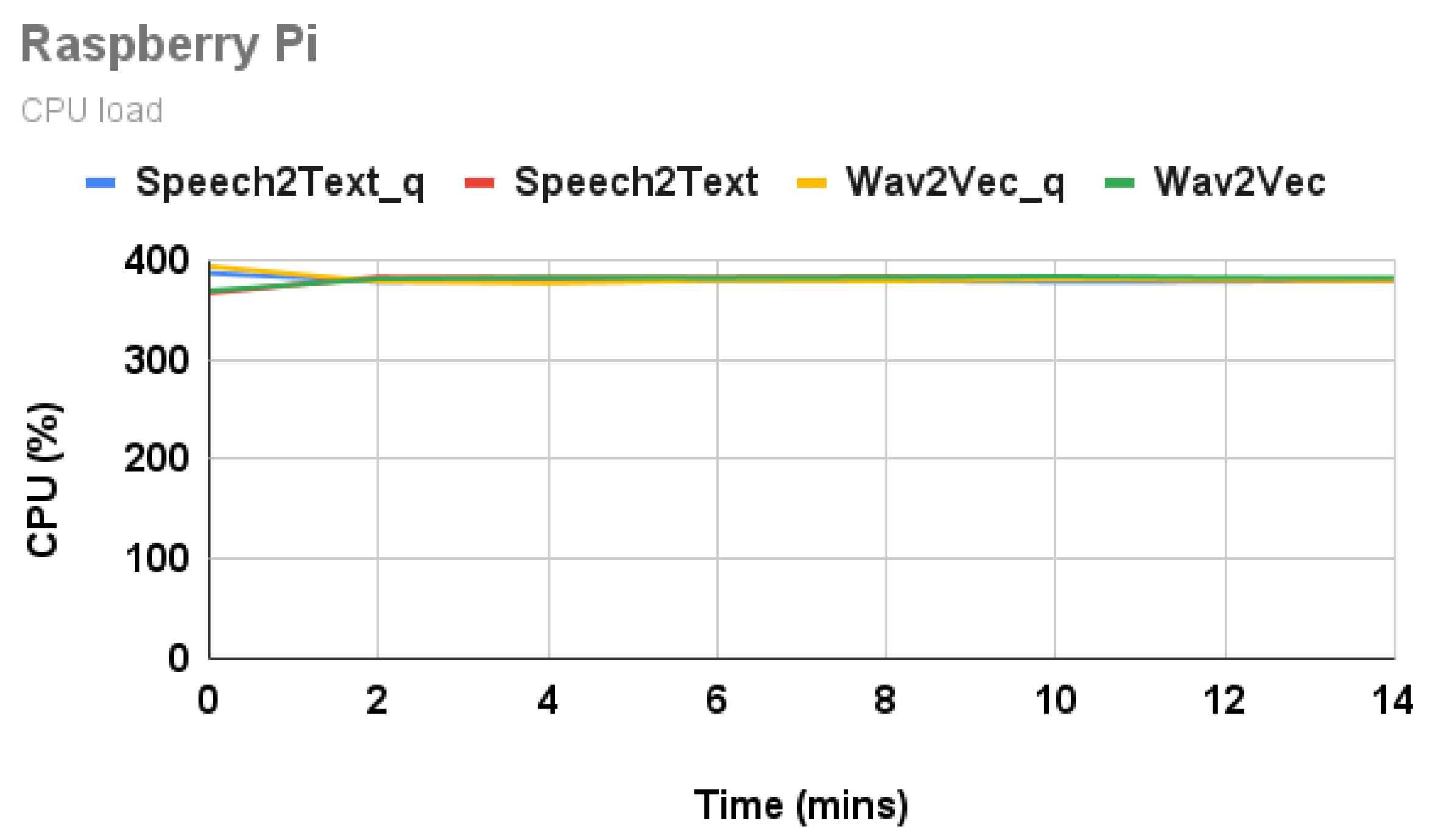
4.3.1. CPU Load

Figure 4 and Figure 5 show the CPU load of all model inferences on Raspberry Pi and Jetson Nano, respectively. The CPU load in Nano for both the Speech2Text and Wav2Vec models is ∼85% in steady state. It mostly uses one of the four cores during operation. Most of the CPU processing on Nano is for copying the input to memory for GPU processing and also copying back the output. On Raspberry Pi, the CPU load is ∼380%. Since all the tensor computations happen on CPU, all CPU cores are utilized fully during model inference. On Nano, the initial few minutes are spent loading and benchmarking the model. That is why the CPU is not busy during the initial few minutes.

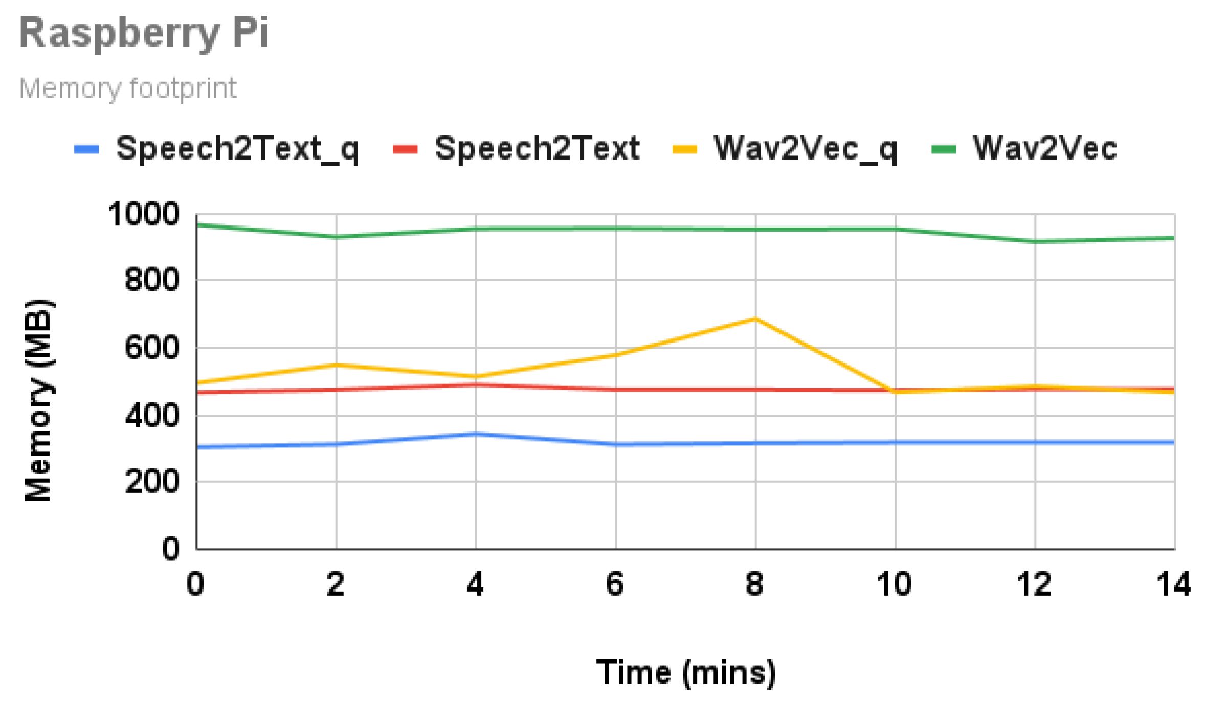
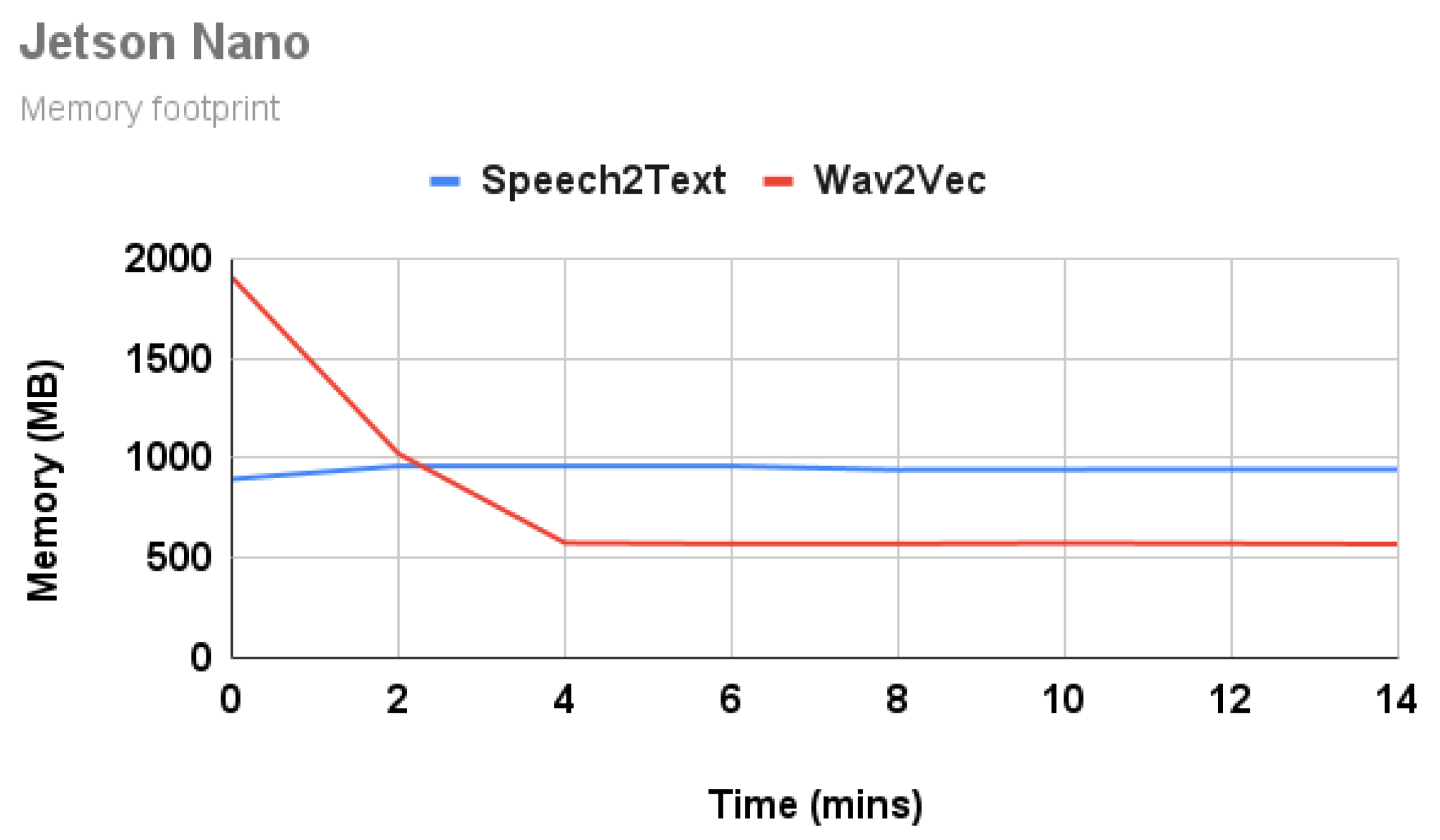
4.3.2. Memory Footprint

Figure 6 and Figure 7 show the memory of all model inferences on Raspberry Pi and Jetson Nano, respectively. The memory values presented here are RES (resident set size) values from top command. On Raspberry Pi, the quantized Wav2Vec model consumes ∼50% less memory (from 1 GB to 560 MB), compared to the unquantized model. Similarly, the Speech2Text model consumes ∼40% less memory (from 480 MB to 320 MB), compared to the unquantized model. On Nano, memory consumption for the Speech2Text model is ∼1 GB, and the Wav2Vec model is ∼500 MB. On Nano, the same memory is shared between GPU and CPU.

4.3.3. Model Load Time

Table 8. Model load times.

Raspberry Pi		Jetson Nano
Model	Avg (sec)	Model	Avg (sec)
Speech2Text	1.4	Speech2Text	24.2
Speech2Text quantized	1.07	Wav2Vec	33.5
Wav2Vec	1.9
Wav2Vec quantized	1.9

shows the model load times on Raspberry Pi and Jetson Nano. A load time of 1–2 s on Raspberry Pi seems reasonable for any practical application where the model is loaded once and the process inference requests multiple times. The load time on Nano is 15–20 times longer than on Raspberry Pi. Nano cuDNN has to allot some amount of cache for loading the model, which takes time.

4.4. PyTorch Profiler

PyTorch profiler (https://pytorch.org/tutorials/recipes/recipes/profiler_recipe.html (accessed on 30 October 2021)) can be used to study the time and memory consumption of the model’s operators. It is enabled through Context Manager in Python. The profiler is used to understand the distribution of CPU percentage over model operations. Some of the columns from the profiler are not shown in the table for simplicity.

4.4.1. Jetson Nano Profiles

Table 9. Jetson Nano profile for the Wav2Vec model.

Name	Self CPU %	Self CUDA	Self CUDA %	# of Calls
forward	0.70	5.373 ms	0.51	1
aten::conv1d	0.14	576.000 us	0.05	8
aten::convolution	0.10	228.000 us	0.02	8
aten::_convolution	0.11	459.000 us	0.04	8
aten::cudnn_convolution	0.32	527.416 ms	50.32	8
<foward op>	0.63	1.054 ms	0.10	61
aten::matmul	0.97	1.614 ms	0.15	98
aten::linear	10.48	1.279 ms	0.12	74
aten::mm	0.84	207.371 ms	19.78	74
aten::to	38.43	185.175 ms	17.67	3
aten::bmm	0.31	20.066 ms	1.91	24
aten::gelu	0.27	20.261 ms	1.93	20
aten::group_norm	0.03	4.000 us	0.00	1
aten::native_group_norm	0.03	19.968 ms	1.90	1
aten::add_	0.8	16.373 ms	1.56	75

and

Table 10. Jetson Nano profile for Speech2Text model.

Name	Self CPU %	Self CUDA	Self CUDA %	# of Calls
forward	6.21	307.304 ms	14.28	1
aten::linear	3.12	86.356 ms	4.01	672
aten::matmul	3.16	80.340 ms	3.73	672
aten::mm	4.72	265.171 ms	12.32	672
aten::layer_norm	1.01	20.434 ms	0.95	253
aten::transpose	5.46	106.751 ms	4.96	1398
aten::native_layer_norm	2.77	91.685 ms	4.26	253
aten::t	2.93	57.888 ms	2.69	710
aten::view	9.56	119.122 ms	5.53	2724
aten::empty	8.34	102.937 ms	4.78	2417
aten::bmm	2.26	83.940 ms	3.90	312
aten::as_strided	6.86	77.660 ms	3.61	2156
aten::add_	4.07	67.874 ms	3.15	675
aten::softmax	0.66	16.265 ms	0.76	156
aten::to	2.38	41.231 ms	1.92	433

show the profiles of Wav2Vec and Speech2Text models on Jetson Nano.

For Wav2Vec model, the majority of the CUDA time is spent in aten::cudnn_convolution for input convolutions followed by matrix multiplication (aten::mm). Additionally, the CPU and GPU spend a significant amount of time transferring data between each other, aten::to.

For the Speech2Text model, the majority of the CUDA time is spent in decoder forward followed by aten::mm for tensor multiplication operations.

4.4.2. Raspberry Pi profiles

Table 11. Raspberry Pi profile for Wav2Vec quantized on model.

Name	Self CPU %	Self CPU	CPU Total	# of Calls
forward	0.49	45.452 ms	9.334 s	1
quantized::linear_dynamic	30.77	2.872 s	3.167 s	74
aten::conv1d	0.00	347.000 us	2.875 s	8
aten::convolution	0.00	274.000 us	2.875 s	8
aten::_convolution	0.02	1.472 ms	2.875 s	8
aten::_convolution_nogroup	0.04	3.663 ms	2.862 s	23
aten::thnn_conv2d	0.30	28.075 ms	2.858 s	23
aten::thnn_conv2d_forward	5.46	509.250 ms	2.830 s	23
aten::addmm_	24.79	2.314 s	2.314 s	23
aten::matmul	0.02	2.316 ms	1.022 s	24
aten::bmm	10.66	994.810 ms	1.016 s	24
aten::gelu	10.33	964.418 ms	965.023 ms	20
aten::softmax	0.01	597.000 us	719.717 ms	12
aten::_softmax	7.69	718.238 ms	719.120 ms	12
aten::mul	2.78	259.586 ms	260.482 ms	12

,

Table 12. Raspberry Pi profile for Wav2Vec non-quantized model.

Name	Self CPU %	Self CPU	CPU Total	# of Calls
forward	0.41	58.280 ms	14.227 s	1
prepacked::linear_clamp_run	54.85	7.804 s	7.994 s	74
aten::conv1d	0.00	388.000 us	2.865 s	8
aten::convolution	0.00	266.000 us	2.865 s	8
aten::_convolution	0.01	1.790 ms	2.865 s	8
aten::_convolution_nogroup	0.01	813.000 us	2.855 s	23
aten::thnn_conv2d	0.20	28.328 ms	2.854 s	23
aten::thnn_conv2d_forward	3.18	452.048 ms	2.826 s	23
aten::addmm_	16.63	2.366 s	2.366 s	23
aten::matmul	0.02	2.350 ms	1.118 s	24
aten::bmm	7.64	1.087 s	1.113 s	24
aten::gelu	6.54	930.477 ms	931.136 ms	20
aten::softmax	0.00	645.000 us	637.379 ms	12
aten::_softmax	4.47	635.864 ms	636.734 ms	12
aten::mul	2.43	345.998 ms	346.924 ms	12

,

Table 13. Raspberry Pi profile for Speech2Text quantized model.

Name	Self CPU %	Self CPU	CPU Total	# of Calls
forward	6.75	237.950 ms	3.527 s	1
quantized::linear_dynamic	29.46	1.039 s	1.634 s	1995
aten::bmm	14.56	513.414 ms	654.848 ms	960
aten::min	7.41	261.352 ms	282.381 ms	1995
aten::max	5.30	186.852 ms	204.806 ms	1996
aten::select	3.11	109.748 ms	158.923 ms	12,591
aten::clamp_min	2.18	76.946 ms	150.032 ms	492
aten::layer_norm	0.45	15.811 ms	122.822 ms	766
aten::softmax	0.18	6.385 ms	114.797 ms	480
aten::_softmax	2.95	104.130 ms	108.412 ms	480
aten::native_layer_norm	2.45	86.478 ms	107.011 ms	766
aten::add	3.01	106.317 ms	106.365 ms	924
aten::relu	0.11	3.752 ms	82.349 ms	246
aten::copy_	2.17	76.565 ms	76.565 ms	1073
aten::empty	1.94	68.404 ms	68.404 ms	11,944

and

Table 14. Raspberry Pi profile for Speech2Text non-quantized model.

Name	Self CPU %	Self CPU	CPU Total	# of Calls
forward	7.93	287.466 ms	3.623 s	1
prepacked::linear_clamp_run	38.51	1.395 s	1.683 s	1995
aten::bmm	11.84	428.876 ms	575.170 ms	960
aten::copy_	10.07	364.827 ms	364.827 ms	3068
aten::select	3.13	113.435 ms	163.539 ms	12591
aten::clamp_min	2.28	82.503 ms	159.938 ms	492
aten::layer_norm	0.49	17.881 ms	150.078 ms	766
aten::native_layer_norm	3.02	109.335 ms	132.197 ms	766
aten::softmax	0.18	6.389 ms	130.655 ms	480
aten::_softmax	3.32	120.186 ms	124.266 ms	480
aten::add	2.81	101.642 ms	101.693 ms	924
aten::relu	0.18	6.374 ms	92.151 ms	246
aten::masked_fill	0.02	640.000 us	79.648 ms	12
aten::mul_	0.35	12.554 ms	79.419 ms	480
aten::mul	1.38	50.079 ms	73.879 ms	560

show the profiles of Wav2Vec and Speech2Text models on Raspberry Pi.

The CPU time is dominated by linear_dynamic for linear layer computations followed by aten::addmm_ for tensor add multiplications.

Compared to the quantized model, the non-quantized model spends 5 s more time in linear computations, prepacked::linear_clamp_run.

CPU percentages are dominated by forward function, linear layer computations and batched matrix multiplication in both quantized and unquantized models.

The unquantized linear layer processing is 40% higher than the quantized version.

5. Conclusions

We evaluated the ASR accuracy, performance and computational efficiency of transformer-based models on edge devices. By applying quantization and PyTorch mobile optimizations for CPU based inferencing, we gain $\sim 10\%$ improvement in latency and ∼50% reduction in the memory footprint at the cost of ∼0.5% increase in WER, compared to the original model. Running the inference on Jetson Nano GPU improves the latency by a factor of 3 to 5. With 1–2 s load times, ∼300 MB of memory footprint and RTF < 1.0, the latest transformer models can be used on typical edge devices for private, secure, reliable and always-available ASR processing. For applications such as dictation, smart home control, accessibility, etc., a small trade off in WER for latency and efficiency gains is mostly acceptable since small ASR errors will not hamper the overall task completion rate for voice commands, such as turning off a lamp, opening an app on a device, etc. By offloading inference to a general purpose GPU, we can potentially gain 3–5× latency improvements.

In future, we are planning to explore other optimization techniques, such as pruning, sparsity, 4-bit quantization and different model architectures to further analyze the WER vs. performance trade offs. We also plan to measure the thermal and battery impact of various models in CPU and GPU platforms on mobile and wearable devices.

References

- Hinton, G.; Deng, L.; Yu, D.; Dahl, G.E.; Mohamed, A.R.; Jaitly, N.; Senior, A.; Vanhoucke, V.; Nguyen, P.; Sainath, T.N.; et al. Deep Neural Networks for Acoustic Modeling in Speech Recognition: The Shared Views of Four Research Groups. IEEE Signal Process. Mag. 2012, 29, 82–97. [Google Scholar] [CrossRef]
- LeCun, Y.; Bengio, Y.; Hinton, G. Deep learning. Nature 2015, 521, 436–444. [Google Scholar] [CrossRef] [PubMed]
- Hannun, A. The History of Speech Recognition to the Year 2030. arXiv 2021, arXiv:2108.00084. [Google Scholar]
- Wu, C.J.; Brooks, D.; Chen, K.; Chen, D.; Choudhury, S.; Dukhan, M.; Hazelwood, K.; Isaac, E.; Jia, Y.; Jia, B.; et al. Machine Learning at Facebook: Understanding Inference at the Edge. In Proceedings of the 2019 IEEE International Symposium on High Performance Computer Architecture (HPCA), Washington, DC, USA, 16–20 February 2019; pp. 331–344. [Google Scholar] [CrossRef]
- Apple A12. Available online: https://en.wikipedia.org/wiki/Apple_A12 (accessed on 30 October 2021).
- Pixel 6. Available online: https://en.wikipedia.org/wiki/Pixel_6 (accessed on 30 October 2021).
- Huggins-Daines, D.; Kumar, M.; Chan, A.; Black, A.; Ravishankar, M.; Rudnicky, A.I. Pocketsphinx: A Free, Real-Time Continuous Speech Recognition System for Hand-Held Devices. In Proceedings of the 2006 IEEE International Conference on Acoustics Speech and Signal Processing Proceedings, Toulouse, France, 14–19 May 2006; Volume 1, p. I. [Google Scholar]
- Peinl, R.; Rizk, B.; Szabad, R. Open Source Speech Recognition on Edge Devices. In Proceedings of the 2020 10th International Conference on Advanced Computer Information Technologies (ACIT), Deggendorf, Germany, 13–15 May 2020; pp. 441–445. [Google Scholar] [CrossRef]
- Hannun, A.; Case, C.; Casper, J.; Catanzaro, B.; Diamos, G.; Elsen, E.; Prenger, R.; Satheesh, S.; Sengupta, S.; Coates, A.; et al. Deep Speech: Scaling up end-to-end speech recognition. arXiv 2014, arXiv:1412.5567. [Google Scholar]
- Povey, D.; Ghoshal, A.; Boulianne, G.; Burget, L.; Glembek, O.; Goel, N.; Hannemann, M.; Motlicek, P.; Qian, Y.; Schwarz, P.; et al. The Kaldi Speech Recognition Toolkit. In Proceedings of the IEEE 2011 Workshop on Automatic Speech Recognition and Understanding, Waikoloa, HI, USA, 11–15 December 2011. [Google Scholar]
- Pratap, V.; Hannun, A.; Xu, Q.; Cai, J.; Kahn, J.; Synnaeve, G.; Liptchinsky, V.; Collobert, R. Wav2Letter++: A Fast Open-source Speech Recognition System. In Proceedings of the ICASSP 2019—2019 IEEE International Conference on Acoustics, Speech and Signal Processing (ICASSP), Brighton, UK, 12–17 May 2019; pp. 6460–6464. [Google Scholar] [CrossRef] [Green Version]
- Lee, J.; Chirkov, N.; Ignasheva, E.; Pisarchyk, Y.; Shieh, M.; Riccardi, F.; Sarokin, R.; Kulik, A.; Grundmann, M. On-Device Neural Net Inference with Mobile GPUs. arXiv 2019, arXiv:1907.01989. [Google Scholar]
- Hadidi, R.; Cao, J.; Xie, Y.; Asgari, B.; Krishna, T.; Kim, H. Characterizing the Deployment of Deep Neural Networks on Commercial Edge Devices. In Proceedings of the 2019 IEEE International Symposium on Workload Characterization (IISWC), Orlando, FL, USA, 3–5 November 2019; pp. 35–48. [Google Scholar] [CrossRef]
- Rabiner, L. A tutorial on hidden Markov models and selected applications in speech recognition. Proc. IEEE 1989, 77, 257–286. [Google Scholar] [CrossRef]
- Juang, B.H.; Levinson, S.; Sondhi, M. Maximum likelihood estimation for multivariate mixture observations of markov chains (Corresp.). IEEE Trans. Inf. Theory 1986, 32, 307–309. [Google Scholar] [CrossRef]
- Mohamed, A.R.; Sainath, T.N.; Dahl, G.; Ramabhadran, B.; Hinton, G.E.; Picheny, M.A. Deep Belief Networks using discriminative features for phone recognition. In Proceedings of the 2011 IEEE International Conference on Acoustics, Speech and Signal Processing (ICASSP), Prague, Czech Republic, 22–27 May 2011; pp. 5060–5063. [Google Scholar] [CrossRef] [Green Version]
- Gu, J.; Wang, Z.; Kuen, J.; Ma, L.; Shahroudy, A.; Shuai, B.; Liu, T.; Wang, X.; Wang, L.; Wang, G.; et al. Recent Advances in Convolutional Neural Networks. Pattern Recognit. 2017, 77, 354–377. [Google Scholar] [CrossRef] [Green Version]
- Abdel-Hamid, O.; Mohamed, A.R.; Jiang, H.; Deng, L.; Penn, G.; Yu, D. Convolutional Neural Networks for Speech Recognition. IEEE/ACM Trans. Audio Speech Lang. Process. 2014, 22, 1533–1545. [Google Scholar] [CrossRef] [Green Version]
- Graves, A. Sequence Transduction with Recurrent Neural Networks. arXiv 2012, arXiv:1211.3711. [Google Scholar]
- Graves, A.; Fernández, S.; Gomez, F.; Schmidhuber, J. Connectionist Temporal Classification: Labelling Unsegmented Sequence Data with Recurrent Neural Networks. In Proceedings of the 23rd International Conference on Machine Learning, ICML ’06, Pittsburgh, PA, USA, 25–29 June 2006; Association for Computing Machinery: New York, NY, USA, 2006; pp. 369–376. [Google Scholar] [CrossRef]
- Bahdanau, D.; Cho, K.; Bengio, Y. Neural Machine Translation by Jointly Learning to Align and Translate. arXiv 2016, arXiv:1409.0473. [Google Scholar]
- Vaswani, A.; Shazeer, N.; Parmar, N.; Uszkoreit, J.; Jones, L.; Gomez, A.N.; Kaiser, L.; Polosukhin, I. Attention Is All You Need. In Proceedings of the 31st Conference on Neural Information Processing Systems (NIPS 2017), Long Beach, CA, USA, 4–9 December 2017. [Google Scholar]
- Brown, T.B.; Mann, B.; Ryder, N.; Subbiah, M.; Kaplan, J.; Dhariwal, P.; Neelakantan, A.; Shyam, P.; Sastry, G.; Askell, A.; et al. Language Models are Few-Shot Learners. arXiv 2020, arXiv:2005.14165. [Google Scholar]
- Devlin, J.; Chang, M.W.; Lee, K.; Toutanova, K. BERT: Pre-training of Deep Bidirectional Transformers for Language Understanding. arXiv 2018, arXiv:1810.04805. [Google Scholar]
- Senior, A.W.; Evans, R.; Jumper, J.; Kirkpatrick, J.; Sifre, L.; Green, T.; Qin, C.; Žídek, A.; Nelson, A.W.R.; Bridgland, A.; et al. Improved protein structure prediction using potentials from deep learning. Nature 2020, 577, 706–710. [Google Scholar] [CrossRef] [PubMed]
- Greff, K.; Srivastava, R.K.; Koutnik, J.; Steunebrink, B.R.; Schmidhuber, J. LSTM: A Search Space Odyssey. IEEE Trans. Neural Netw. Learn. Syst. 2017, 28, 2222–2232. [Google Scholar] [CrossRef] [PubMed] [Green Version]
- Baevski, A.; Zhou, H.; Mohamed, A.; Auli, M. wav2vec 2.0: A Framework for Self-Supervised Learning of Speech Representations. arXiv 2020, arXiv:2006.11477. [Google Scholar]
- Wang, C.; Tang, Y.; Ma, X.; Wu, A.; Okhonko, D.; Pino, J. fairseq S2T: Fast Speech-to-Text Modeling with fairseq. In Proceedings of the 2020 Conference of the Asian Chapter of the Association for Computational Linguistics (AACL), System Demonstrations, Suzhou, China, 4–7 December 2020. [Google Scholar]
- Droppo, J.; Acero, A. 33. Environmental Robustness. Available online: http://ai.stanford.edu/~amaas/data/cmn_paper.pdf (accessed on 30 October 2021).
- Muda, L.; Begam, M.; Elamvazuthi, I. Voice Recognition Algorithms using Mel Frequency Cepstral Coefficient (MFCC) and Dynamic Time Warping (DTW) Techniques. arXiv 2010, arXiv:1003.4083. [Google Scholar]
- Panayotov, V.; Chen, G.; Povey, D.; Khudanpur, S. Librispeech: An ASR corpus based on public domain audio books. In Proceedings of the 2015 IEEE International Conference on Acoustics, Speech and Signal Processing (ICASSP), South Brisbane, Australia, 19–24 April 2015; pp. 5206–5210. [Google Scholar] [CrossRef]
Figure 1.
Wav2Vec2 inference.
Figure 2.
Speech2Text inference.
Figure 3.
Model preparation steps.
Figure 4.
CPU load on Raspberry Pi.
Figure 5.
CPU load on Jetson Nano.
Figure 6.
Memory footprint on Raspberry Pi.
Figure 7.
Memory footprint on Jetson Nano.