Technoeconomic and Environmental Study of Multi-Objective Integration of PV/Wind-Based DGs Considering Uncertainty of System

Abstract

For technological, economic, and environmental reasons, renewable distributed generators (RDGs) have been extensively used in distribution networks. This paper presents an effective approach for technoeconomic analysis of optimal allocation of REDGs considering the uncertainties of the system. The primary issue with renewable-based distributed generators, especially wind and photovoltaic systems, is their intermittent characteristic that results in fluctuating output power and, hence, increasing power system uncertainty. Thus, it is essential to consider the uncertainty of such resources while selecting their optimal allocation within the grid. The main contribution of this study is to figure out the optimal size and location for RDGs in radial distribution systems while considering the uncertainty of load demand and RDG output power. A Monte Carlo simulation approach and a backward reduction algorithm were used to generate a reasonable number of scenarios to reflect the uncertainties of loading and RDG output power. Manta ray foraging optimization (MRFO), an efficient technique, was used to estimate the ratings and placements of the RDGs for a multi-objective function that includes the minimization of the expected total cost, total emissions, and total system voltage deviation, in addition to enhancing predicted total voltage stability. An IEEE 118-bus network was used as a large interconnected network, along with a rural 51-bus distribution grid and the IEEE 15-bus model as a small distribution network to test the developed technique. Simulations demonstrate that the proposed optimization technique effectively addresses the optimal DG allocation problem. Furthermore, the results indicate that using the proposed method to optimally integrate wind turbines with solar-based DG decreases the expected costs, emissions, and voltage deviations while improving voltage stability by 40.27%, 62.6%, 29.33%, and 4.76%, respectively, for the IEEE 118-bus system and enhances the same parameters by 35.57%, 59.92%, 68.95%, and 11.88%, respectively, for the rural 51-bus system and by 37.74%, 61.46%, 58.39%, and 8.86%, respectively, for the 15-bus system.

1. Introduction

1.1. Problem Statement

Uncertainty is a key issue in determining the best size and position for distributed generators (DGs) in electrical systems, and it is a big contributor to the problem’s complexity, especially when it comes to load demand and renewable energy resources (RERs).

While much effort has been conducted to optimize the integration of DGs within electricity grids, few studies accounted for uncertainty. The optimal allocation of wind turbine (WT) and photovoltaic (PV) systems within grids, along with the consideration of system uncertainty, plays a key role in maintaining system reliability. Electric power producers often employ DGs close to the load center for economic, technical, and environmental reasons. Integration of distributed renewable energy sources such as wind and photovoltaic within power systems has increased significantly over the last few years. Due to the intermittent characteristics of solar irradiance and wind speed, the output power of such systems exhibits continuous fluctuations, which contributes to the uncertainty of electric power systems. Thus, for optimal renewable distributed generator (RDG) sizing and location, the uncertainties of the system should be considered.

1.2. Literature Review

The fundamental purpose of DGs is to provide proper distribution network operation with reduced system losses, improved voltage profile, and higher system reliability [1]. DGs are now a clean and cost-effective source of energy, and RER production rates have recently fallen, despite the fact that the cost of generating electricity using traditional generators is rapidly increasing due to the rise of the fuel cost [2,3]. Lowering energy costs, reducing emissions, and improving voltage profiles are all advantages of a proper optimal DG allocation [4,5,6]. However, because of the uncertain nature of RERs, improper DG placement can cause system instability and voltage fluctuations [7,8]. The topic of optimal DG integration has been discussed in a number of studies from various perspectives. The firefly algorithm (FA) and particle swarm optimization (PSO) method were presented in [9] to achieve techno-economic and environmental benefits in electrical distribution networks. A PSO and hybrid enhanced gray wolf optimizer (EGWO-PSO) approach was presented in [10] for the optimal DG allocation in order to reduce system costs, emissions, active power losses, and voltage deviation index (VDI), as well as increase voltage stability index (VSI). For electrical power planning with load uncertainties, the authors of [11] suggested a Monte Carlo simulation-based bioinspired algorithm. To reduce the overall energy loss when sizing and deploying DG units, a method known as coefficient particle swarm optimization (CPSO) was used in [12]. In [13], the Salp swarm optimizer (SSO) was combined with the PSO method to improve the technical–economical–environmental performance of power plants. The authors of [14] introduced the equilibrium optimizer (EO) method, an efficient algorithm for solving the micro-grid energy management problem and optimizing the DG size and location within power systems. Monte Carlo simulation was employed in [15] for optimum DG allocation. The authors of [16] suggested a bilayer optimization technique for optimal battery energy storage system (BESS) and solar photovoltaic (SPVs) placement in the distribution system. In [17], a solution called strength Pareto evolutionary algorithm 2 (SPEA2) was presented for tackling the DGs and capacitor placement problem with load uncertainty. The manta ray foraging optimization algorithm (MRFOA) was proposed in [18] for the best control and operation of distribution networks with the least amount of lost energy. The manta ray foraging optimizer (MRFO) is a new and effective bioinspired algorithm for engineering applications that simulates the intelligent foraging behavior of manta rays in the environment [19]. The MRFO is used in this paper to determine the optimal solar and wind system allocation in a network based on IEEE 118-bus, rural 51-bus, and IEEE 15-bus systems for minimizing the expected total cost, emissions, and voltage deviation, and enhancing voltage stability while taking into account the uncertainties of load demand and solar and wind power generation.

1.3. Contribution of the Paper

The uncertainty of the RER output power and load demand is considered the most challenging issue related to optimal sizing and allocation of RDGs within power grids. As a result of the continuous increase in the penetration level of the RER to the power grids, the problem has grown significantly, forcing the construction of a more efficient solution. This paper is aimed at solving the optimal allocation of RDGs problem in a distribution system using a backward reduction technique that takes into account uncertainties due to load demand and RER. The contributions of the paper can be summarized as follows:

• Presenting an effective backward reduction strategy to solve the optimal distribution system problem sizing and placement,
• Addressing the issue of the load and RER output power uncertainties,
• Adopting a Monte Carlo simulation approach and backward reduction algorithm to model electrical system uncertainty,
• Employing MRFO algorithm to solve the problem using the IEEE 118-bus, rural 51-bus, and the IEEE 15-bus distribution systems,
• Comparing the performance of MRFO with several well-known problem-solving algorithms.

2. Problem Formulation

Four objective functions were studied as part of a multi-objective function in this paper [20,21]. It is worth noting that, while modeling or assessing power system uncertainty, various scenarios must be considered. Each scenario has its own set of expected values, as elaborated below.

2.1. Proposed Objective Functions

2.1.1. Minimizing the Total Expected Cost ($ETCost$)

The total annual expected cost ($ETCost$) includes the cost of the main substation’s electric energy saving ($ECos{t}_{Grid}$), cost of the integrated PV ($ECos{t}_{PV}$), and cost of the WT ($ECos{t}_{WT}$), expressed as

$$ETCost=ECos{t}_{Grid}+ECos{t}_{PV}+ECos{t}_{WT}.$$

(1)

The detailed items of Equation (1) are defined as follows:

$$ETCos{t}_{Grid}={\displaystyle \sum }_{k=1}^{Ns}ECos{t}_{Grid,k}={\displaystyle \sum }_{k=1}^{Ns}Cos{t}_{Grid,k}\times {\pi }_{S,k},$$

(2)

$$Cos{t}_{Grid}=P_{Grid}\times K_{Grid},$$

(3)

$$ETCos{t}_{PV}={\displaystyle \sum }_{k=1}^{Ns}ECos{t}_{PV,k}={\displaystyle \sum }_{k=1}^{Ns}{\pi }_{Solar,k}\times \left(a_{PV}+b_{PV}\times P{G}_{PV}\right),$$

(4)

$$a_{PV}=\frac{capital cost\text{\_}PV\times P_{sr}\times Gr}{life time\text{\_}PV\times 8760\times LF},$$

(5)

$$b_{PV}=Cost\text{\_}P{V}_{O\&M}+Cost\text{\_}P{V}_{Fuel},$$

(6)

$$ETCos{t}_{wind}={\displaystyle \sum }_{k=1}^{Ns}ECos{t}_{wind,k}={\displaystyle \sum }_{k=1}^{Ns}{\pi }_{wind,k}\times \left(a_{wind}+b_{wind}\times P{G}_{wind}\right),$$

(7)

$$a_{wind}=\frac{capital cost\text{\_}wind\times P_{wr}\times Gr}{life time\text{\_}wind\times 8760\times LF},$$

(8)

$$b_{wind}=Cost\text{\_}win{d}_{O\&M}+Cost\text{\_}win{d}_{Fuel},$$

(9)

where $a_{PV}$ is the annual PV unit installment cost, and $b_{PV}$ is the annual PV unit’s operation and maintenance cost. The annual WT installment cost is $a_2$, and the annual WT operating and maintenance cost is $b_2$. $LF$ is the load factor of DGs, and $Gr$ is the annual rate of benefit (USD/h). The cost coefficients of PV in this study were chosen to be $capital cost\text{\_}PV$ = 3985 USD/kW, $Cost\text{\_}P{V}_{O\&M}$ = 0.01207 USD/kWh, and $Cost\text{\_}P{V}_{Fuel}$ = 0 USD/kWh. The wind cost coefficients were set to $capital cost\text{\_}wind$ = 1822 USD/kW, $Cost\text{\_}win{d}_{O\&M}$ = 0.00952 USD/kWh, and $Cost\text{\_}win{d}_{Fuel}$ = 0 USD/kWh. The operational lifetime of PV and WT was assumed to be 20 years, with $K_{Grid}$ = 0.096 [20].

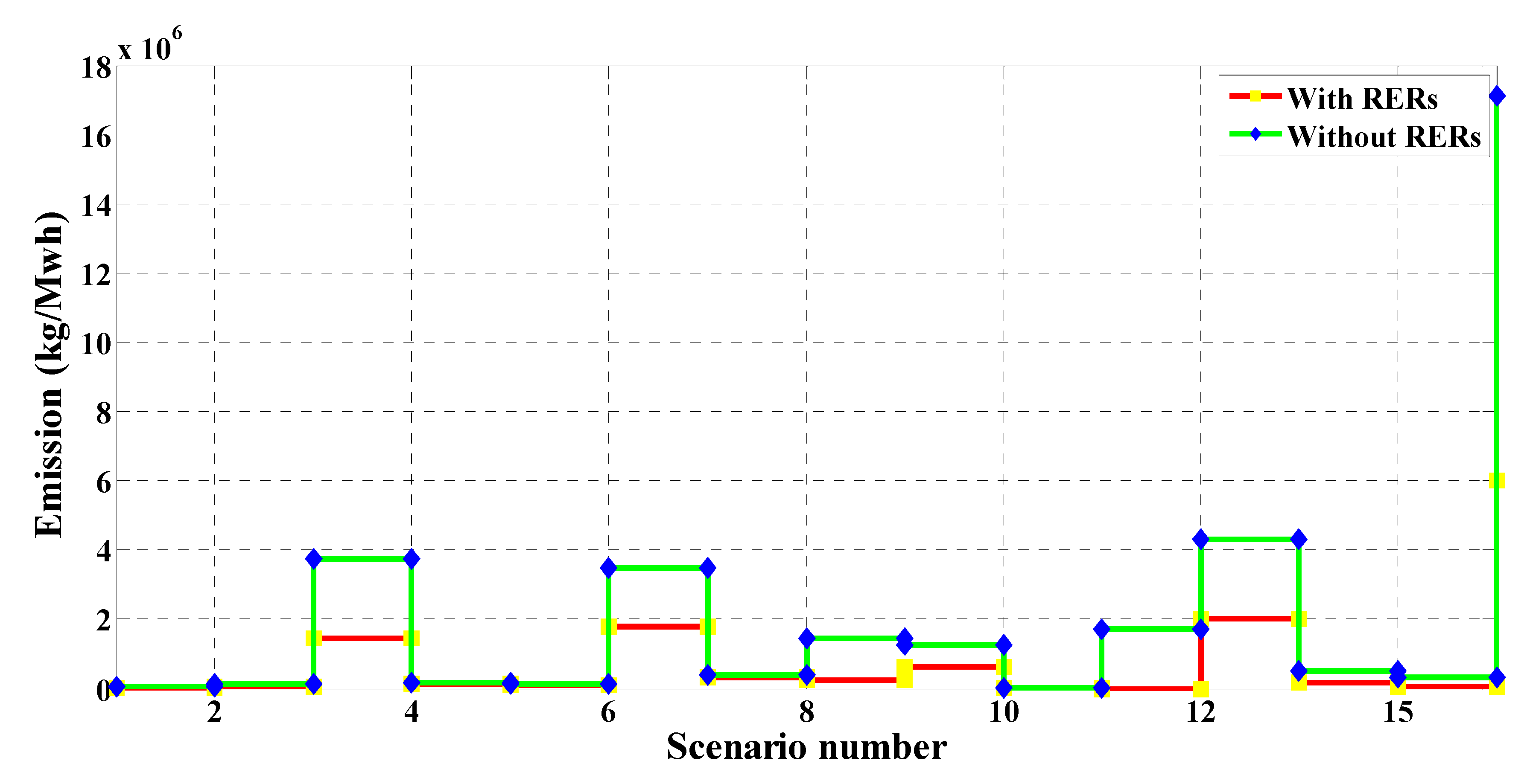
2.1.2. Minimizing the Total Expected Emissions ($ETEmission$)

Carbon dioxide (CO₂), sulfur dioxide (SO₂), and nitrogen oxides (NO_x) are the most effective pollutants resulting from fossil fuels used in thermal power plants. The proposed objective function to minimize the emission of such toxic gases can be formulated as follows [20]:

$$ETEmission={\displaystyle \sum }_{k=1}^{Ns}EEmissio{n}_k={\displaystyle \sum }_{k=1}^{Ns}{\pi }_{Grid,k}\times E_{Grid,k},$$

(10)

$$f_2\left(x\right)={\displaystyle \sum }_{i=1}^{N_{DG}}{E}_{D{G}_i}+E_{Grid},$$

(11)

$$E_{D{G}_i}=\left(C{O}_2^{DG}+N{O}_x^{DG}+S{O}_2^{DG}\right)\times P{G}_i,$$

(12)

$$E_{Grid}=\left(C{O}_2^{Grid}+N{O}_x^{Grid}+S{O}_2^{Grid}\right)\times P_{gGrid},$$

(13)

where $ETEmission$ represents the total expected emission, and f₂ is the emission reduction from generation units. Grid NO_x, SO₂, and CO₂ emission rates were set to 5.06 kg/MWh, 11.6 kg/MWh, and 2031 kg/MWh respectively [20].

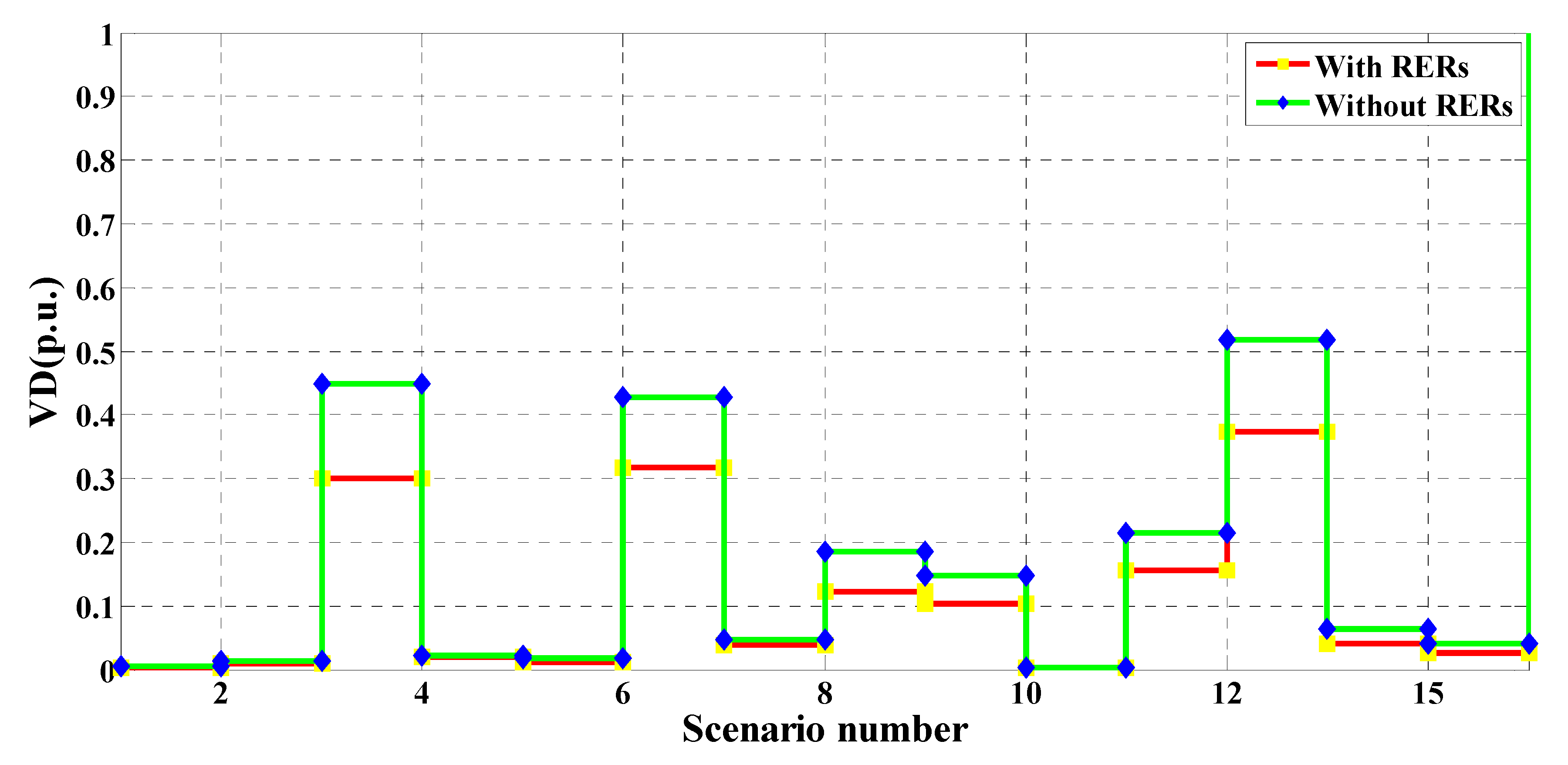
2.1.3. Minimizing the Expected Voltage Deviation (EVD)

The expected total voltage deviation $ETVD$ of a radial distribution network (RDN) is expressed as follows [20,21]:

$$ETVD={\displaystyle \sum }_{L=1}^{Ns}EV{D}_L={\displaystyle \sum }_{L=1}^{Ns}{\pi }_{S,L}\times V{D}_L,$$

(14)

where

$$VD={\displaystyle \sum }_{k=1}^n\left|V_k-1\right|.$$

(15)

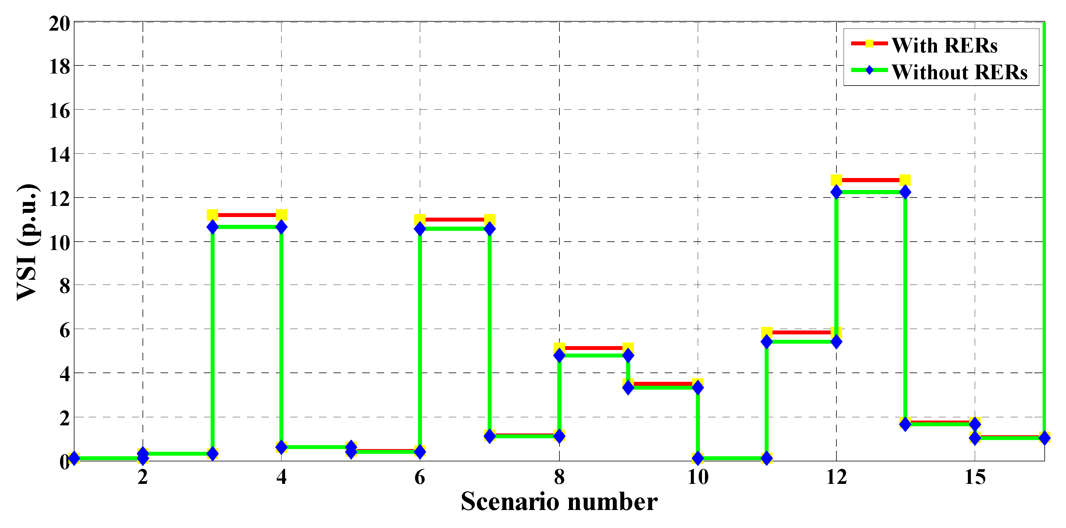
2.1.4. Enhancing the Expected Voltage Stability Index

The sum of the expected voltage stability indexes (ETVSI) can be formulated as

$$ETVSI={\displaystyle \sum }_{L=1}^{Ns}EVS{I}_L={\displaystyle \sum }_{L=1}^{Ns}{\pi }_{S,L}\times VS{I}_L,$$

(16)

$$VS{I}_n={\left|V_n\right|}^4-4{\left(P_n{X}_{nm}-Q_n{R}_{nm}\right)}^2-4\left(P_n{X}_{nm}+Q_n{R}_{nm}\right){\left|V_n\right|}^2.$$

(17)

2.1.5. Proposed Multi-Objective Function

The above objective functions were integrated into a multi-objective function. The weight approach method was utilized to prioritize the goals to be achieved. Furthermore, the objectives should be normalized on the basis of their base value (without WT and PV), to eliminate scaling concerns and make the objective function dimensionless. The multi-objective function F is given by Equation (18).

$$F={\Omega }_1{F}_1+{\Omega }_2{F}_2+{\Omega }_3{F}_3+{\Omega }_4{F}_4$$

(18)

where ${\Omega }_1$, ${\Omega }_2$,${\Omega }_3$, and ${\Omega }_4$ are the weighing factors that should satisfy Equation (19).

$$\left|{\Omega }_1\right|+\left|{\Omega }_2\right|+\left|{\Omega }_3\right|+\left|{\Omega }_4\right|=1$$

(19)

where, ${\Omega }_1$ = ${\Omega }_2$ = ${\Omega }_3$ = ${\Omega }_4$ = 0.25 [20].

The respective normalized objective functions in Equation (18) are calculated as follows:

$$F_1=\frac{ETCost}{ETCos{t}_{base}}$$

(20)

$$F_2=\frac{ETEmission}{ETEmissio{n}_{base}}$$

(21)

$$F_3=\frac{ETVD}{ETV{D}_{base}}$$

(22)

$$F_4=\frac{1}{ETVSI}$$

(23)

2.2. System Constraints

The above multi-objective function is solved subject to the below constraints.

2.2.1. Equality Constraints

The active and reactive powers flow in RDN are included in the equality constraints, which can be written as follows:

$$P_{Grid}+{\displaystyle \sum }_{j=1}^{NPV}{P}_{PV,j}+{\displaystyle \sum }_{j=1}^{NWT}{P}_{WT,j}={\displaystyle \sum }_{j=1}^{NT}{P}_{loss,j}+{\displaystyle \sum }_{j=1}^{NB}{P}_{L,j}.$$

(24)

$$Q_{Grid}+{\displaystyle \sum }_{j=1}^{NT}{Q}_{WT,j}={\displaystyle \sum }_{j=1}^{NT}{Q}_{loss,j}+{\displaystyle \sum }_{j=1}^{NB}{Q}_{L,j}.$$

(25)

2.2.2. Inequality Constraints

The inequality constraints can be given as follows:

$$V_{min}\le V_j\le V_{max}.$$

(26)

$${\displaystyle \sum }_{j=1}^{NWT}{Q}_{WT,j}\le {\displaystyle \sum }_{j=1}^{NB}{Q}_{L,j}.$$

(27)

$$I_n\le I_{max,n} n=1,2,3\dots ,NT.$$

(28)

where, $V_{min}$ and $V_{max}$ are the lower and the upper voltage limits.

3. Uncertainty Modeling of PV, Wind Turbine, and Load Demand

The continuous probability density function (PDF) is used to consider the uncertainty in load demand, WT, and PV systems.

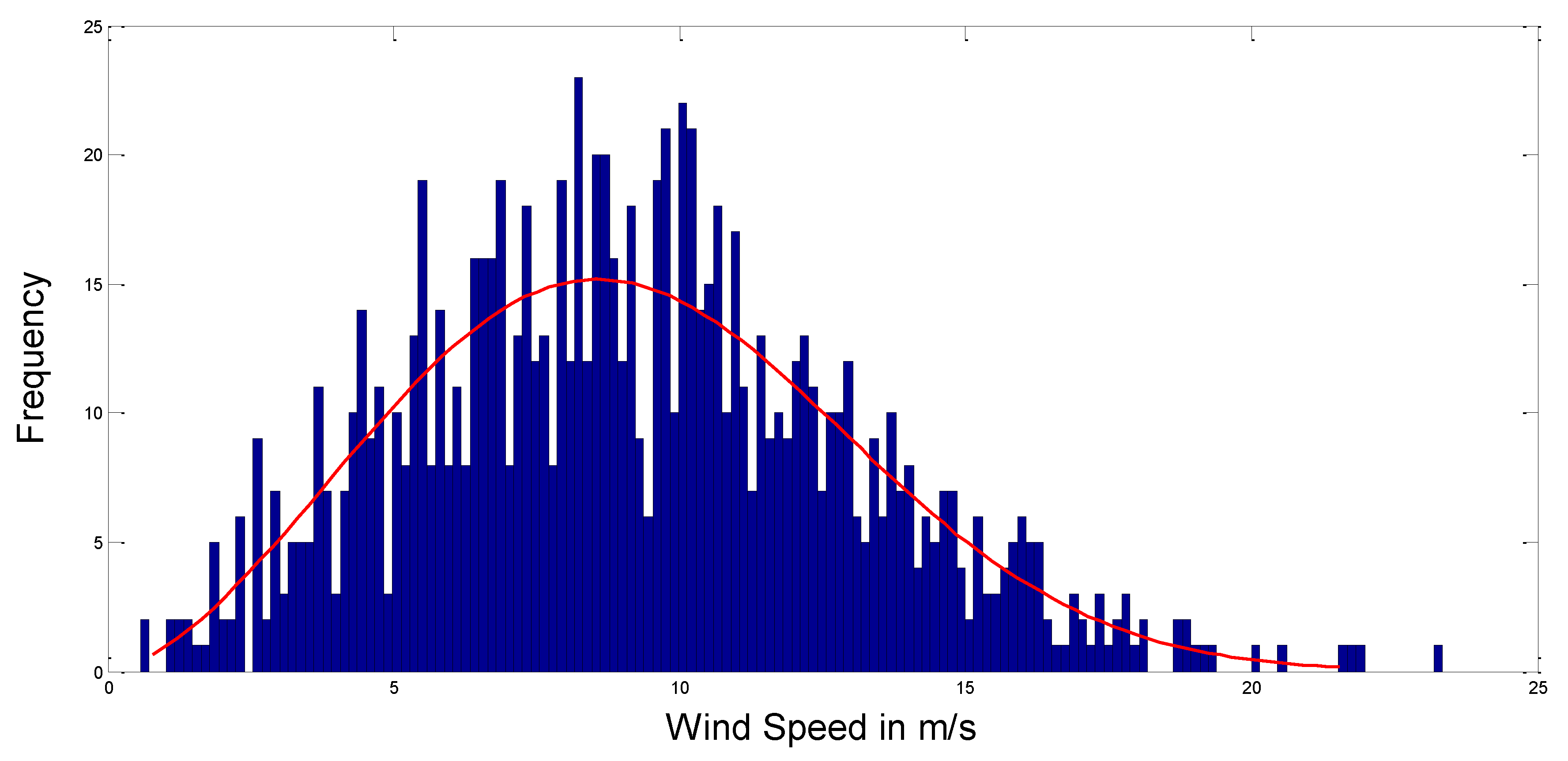
3.1. WT Uncertainty Modeling

Wind speed uncertainty can be modeled using the Weibull PDF given by Equation (29) [22].

$$f_v\left(v\right)=\left(\frac{\beta }{\alpha }\right) {\left(\frac{v}{\alpha }\right)}^{\left(\beta -1\right)} \exp \left[-{\left(\frac{v}{\alpha }\right)}^{\beta }\right] 0\le v<\infty .$$

(29)

The scaling and shaping factors for Weibull PDF are $\alpha , \beta$ that were set to $\alpha$ = 10.5 and $\beta$ = 2.6. A 1000 Monte Carlo wind speed distribution scenario utilizing Weibull PDF is depicted in Figure 1.

The output power of a WT is a function of wind speed expressed as follows [22]:

$$P_{\omega }\left(v_{\omega }\right)=\{\begin{array}{ll}0& for v_{\omega } < v_{\omega i}| v_{\omega } > v_{\omega } \\ P_{\omega r}\left(\frac{v_{\omega }-v_{\omega i}}{v_{\omega r}-v_{\omega i}}\right)& for (v_{\omega i }\le v_{\omega }\le v_{\omega r})\\ P_{\omega r}& for \left( v_{\omega r }\le v_{\omega }\le v_{\omega o}\right)\end{array},$$

(30)

where, $P_{\omega r}$ is the rated output power of the WT, and $v_{\omega i}$ = 3 m/s, $v_{\omega o}$ = 25 m/s, and $v_{\omega r}$ = 16 m/s are the cut-in, cut-out, and rated speed of the WT, respectively.

For each wind scenario, the probability of wind speed is computed using Equation (31).

$${\tau }_{wind, L }={{\displaystyle \int }}_{v_L^{min}}^{v_L^{max}}{f}_v\left(v\right) dv,$$

(31)

where $v_L^{min}$ and $v_L^{max}$ mark the beginning and end of the interval of wind speed for the L-th scenario, and ${\tau }_{wind,L }$ is the probability of WT speed being in the $L$-th scenario.

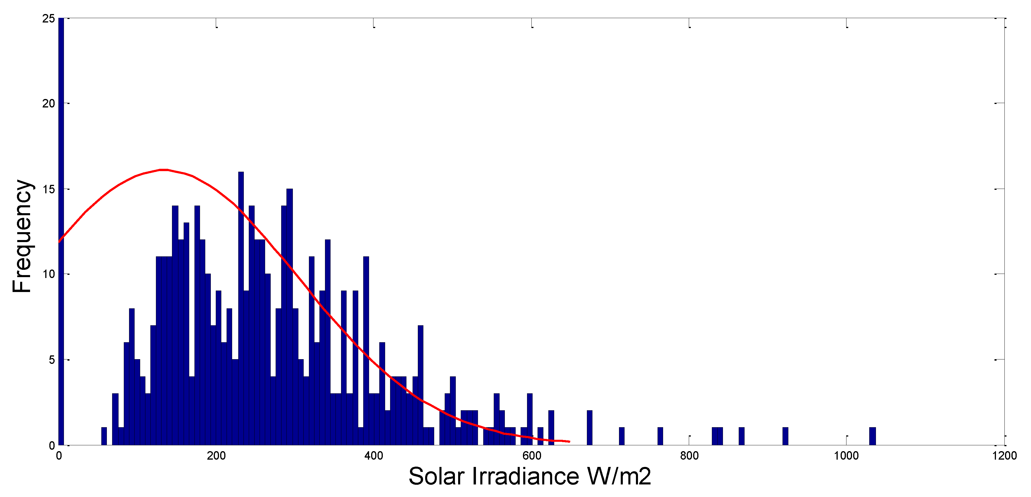
3.2. PV Uncertainty Modeling

The lognormal PDF can be used to specify the solar irradiance uncertainty [23].

$$f_G\left(G\right)=\frac{1}{G {\sigma }_s\sqrt{2\pi }} exp\left[-\frac{{\left(\ln G-{\mu }_s\right)}^2}{2{\sigma }_s{}^2}\right] for G>0,$$

(32)

where ${\mu }_{s,}$ and ${\sigma }_s$ represent the mean and standard deviation of the random variables, which were set to 5.5 and 0.5, respectively [23].

The solar irradiation scenarios using the Monte Carlo simulation are shown in Figure 2.

The output power of a PV array as a function of irradiance can be calculated as follows [22]:

$$P_s\left(G\right)=\{\begin{array}{c}{P}_{sr}\left(\frac{G^2}{G_{std} \times M_c}\right) for 0< G \le M_c\\ P_{sr}\left(\frac{G}{G_{std} }\right) for G \ge M_c\end{array},$$

(33)

where $M_c$ represents a certain irradiance point which is set to 120 W/m², and $G_{std}$ is the standard solar irradiance which is equal to 1000 W/m² [23].

The probability of solar irradiation can be calculated using Equation (34) [23].

$${\tau }_{solar, m }={{\displaystyle \int }}_{G_n^{min}}^{G_n^{max}}{f}_G\left(G\right) dG,$$

(34)

where $G_n^{min}$ and $G_n^{max}$ are the starting and ending points of the solar irradiance interval in the $n$-th scenario.

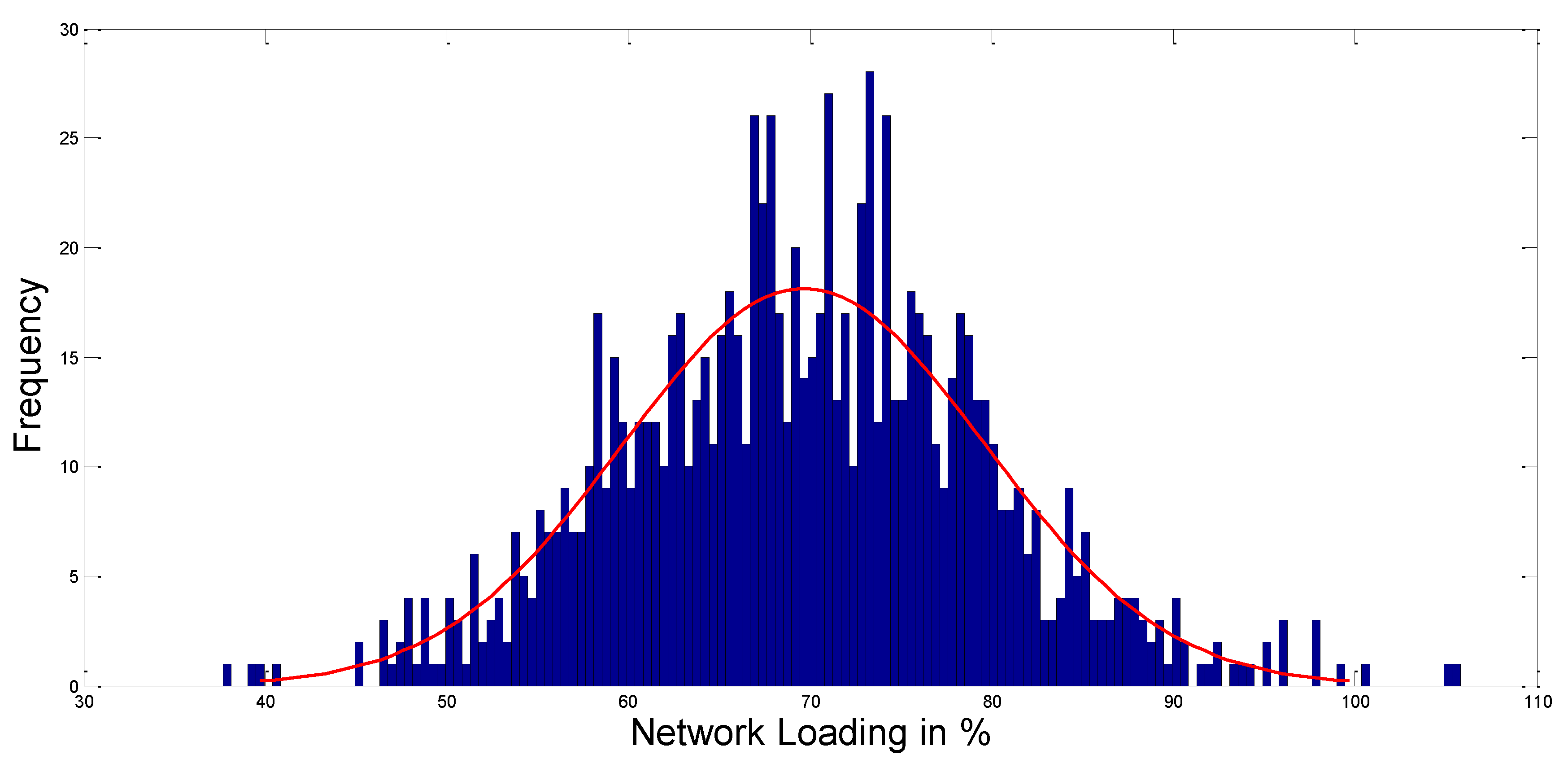
3.3. Load Demand Uncertainty Modeling

The normal distribution PDF can be used to simulate the uncertainty in the load demand as shown below [24].

$$f_d\left(P_d\right)=\frac{1}{ {\sigma }_d\sqrt{2\pi }} exp\left[-\frac{{\left(P_d-{\mu }_d\right)}^2}{2{\sigma }_d{}^2}\right],$$

(35)

where the standard and mean deviation values are ${\sigma }_d$ and ${\mu }_d$, respectively. $P_d$ represents the load normal distribution’s probability density. Figure 3 shows the Monte Carlo scenarios of load demand formed with a normal distribution PDF (${\sigma }_d$ = 10, ${\mu }_d$ = 70, and sample size = 1000).

To calculate the load demand probability and expected load scenarios, the following equations are used [24]:

$${\tau }_{d, i }={{\displaystyle \int }}_{v_{d,i}^{min}}^{v_{d,i}^{max}}\frac{1}{ {\sigma }_d\sqrt{2\pi }} exp\left[-\frac{{\left(P_d-{\mu }_d\right)}^2}{2{\sigma }_d{}^2}\right] d{p}_d,$$

(36)

$$P_{d, i}=\frac{1}{{\tau }_{d, i }}{{\displaystyle \int }}_{P_{d,i}^{min}}^{P_{d,i}^{max}}\frac{P_d}{ {\sigma }_d\sqrt{2\pi }} exp\left[-\frac{{\left(P_d-{\mu }_d\right)}^2}{2{\sigma }_d{}^2}\right] d{p}_d,$$

(37)

where $P_{d,i}^{min}$ and $P_{d,i}^{max}$ represent the border limits of interval $i$.

3.4. Backward Reduction Algorithm

The authors of [21] demonstrated how to use the backward reduction technique to reduce possibilities. The probabilities associated with various scenarios are shown in

Table 1. Reduced created scenarios, with associated uncertainties.

Scenario	${\mathit{\pi }}_{\mathit{s}}$ (Scenario Probability)	Irradiance of PV (W/m2)	Speed of WT (m/s)	Loading %
$\mathrm{S}1$	0.0010	825.1	5.7	82.1
$\mathrm{S}2$	0.0030	665.8	8.1	85.9
$\mathrm{S}3$	0.1050	311.2	9.3	72.8
$\mathrm{S}4$	0.0060	80.3	4.6	58.2
$\mathrm{S}5$	0.0040	744.2	7.1	75.4
$\mathrm{S}6$	0.1040	201.8	7.7	68.4
$\mathrm{S}7$	0.0110	585.5	4.3	73.8
$\mathrm{S}8$	0.0470	360.5	10.6	63.7
$\mathrm{S}9$	0.0330	406.5	8.2	78.1
$\mathrm{S}10$	0.0010	909.6	5.7	64.5
$\mathrm{S}11$	0.0530	250.6	13.6	66.1
$\mathrm{S}12$	0.1210	133.4	8.8	72.9
$\mathrm{S}13$	0.0160	504.8	8.8	64.4
$\mathrm{S}14$	0.0100	455.6	10.3	65.4
$\mathrm{S}15$	0.4850	0	10.3	72.1

. The probability of each scenario, the solar irradiation, the wind speed, and the percentage of loading are listed in the table.

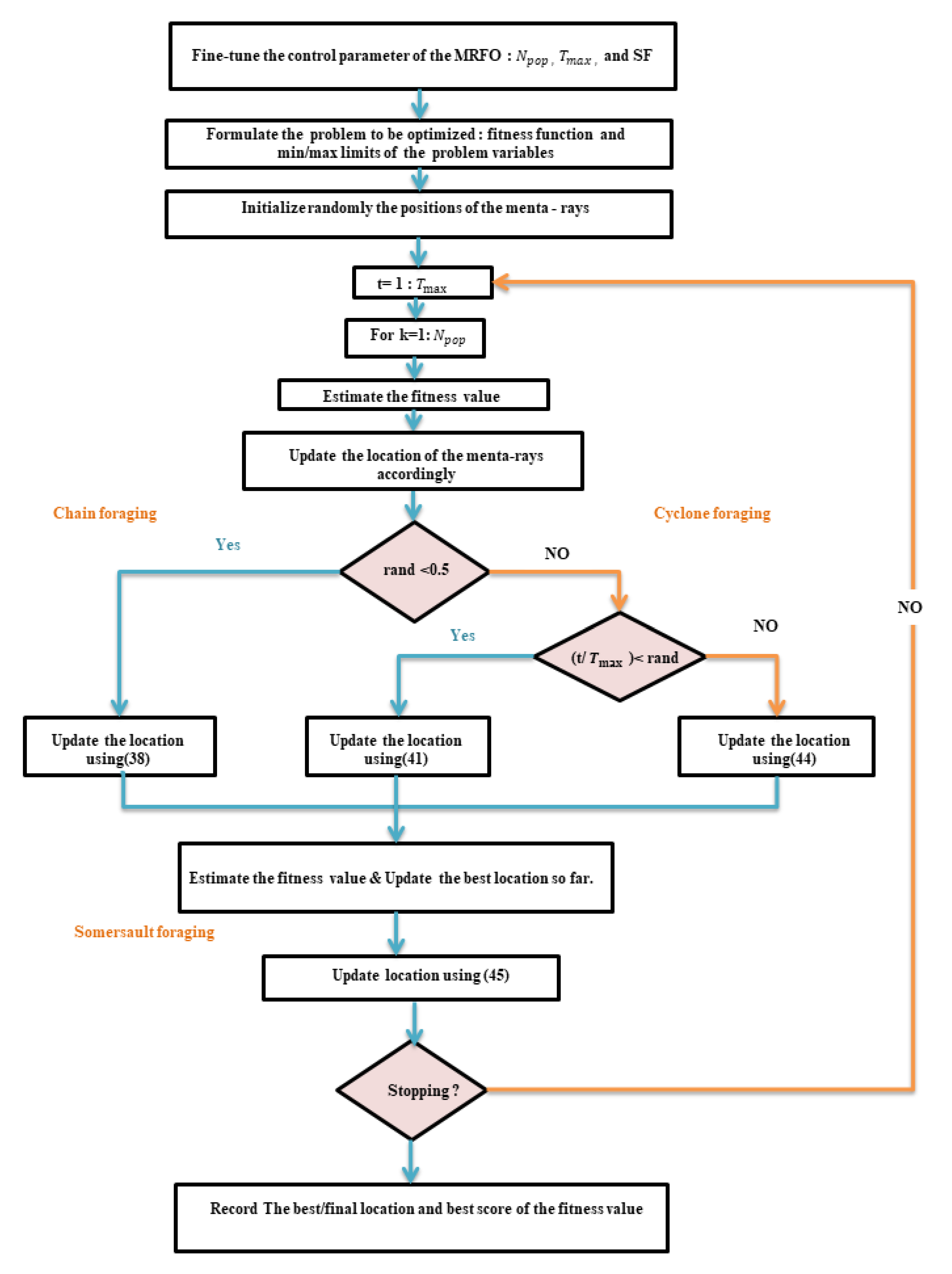
4. Optimization Algorithms

The manta ray foraging optimizer (MRFO) is a new bioinspired optimization technique which was introduced in 2020 for solving engineering applications [19]. Manta rays are aquatic animals with two pectoral fins and a flat body. They are able to swim freely, as if they were birds. They also feature a pair of vertical lobes protruding from their massive terminal jaws. They do not have sharp teeth; therefore, they eat plankton (microscopic animals) [19]. The MRFO is similar to other optimizers that are based on developing the exploration and exploitation stages. For solving distinct optimization issues, three foraging strategies, i.e., chain foraging, cyclone foraging, and somersault foraging, can be used to define the development [25,26,27]. The mathematical models of the three foraging strategies are described below.

4.1. Chain Foraging

Manta rays may be able to identify plankton through MRFO and swim toward it. A larger concentration of plankton in a location results in a better identification process. The mathematical model of chain foraging can be expressed as

$$x_i^b\left(t+1\right)=\{\begin{array}{c}{x}_i^b\left(t\right)+A\ast \left(x_{best}^b\left(t\right)-x_i^b\left(t\right)\right)+\rho \times \left( x_{best}^b\left(t\right)-x_i^b\left(t\right)\right) i=1\\ x_i^b\left(t\right)+A\ast \left(x_{i-1}^b\left(t\right)-x_i^b\left(t\right)\right)+\rho \times \left( x_{best}^b\left(t\right)-x_i^b\left(t\right)\right) i=2, \dots , N\end{array},$$

(38)

$$\rho =2\times A\times \sqrt{\left|\log \left(A\right)\right|},$$

(39)

where $A$ is a random vector within the range [0, 1], $x_i^b\left(t\right)$ is the position of the $i$-th individual at time $t$ in $b$-th dimension, $x_{best}^b\left(t\right)$ is the plankton with the highest concentration, and $\rho$ is a weight coefficient. The position update of the $i$-th individual is determined by the position $x_{i-1}^b\left(t\right)$ of the $\left(i-1\right)$-th current individual and the position $xbest\left(t\right)$ of the food.

4.2. Cyclone Foraging

When manta rays find plankton in deep water, they form a lengthy foraging chain and spiral their way to the food. Each manta ray swims in the same direction following the manta ray in front. Manta rays, in other words, hunt in swarms, spiraling around each other. The mathematical equation that can be used to model manta rays’ spiral-shaped movement in 2D space is

$$\{\begin{array}{c}{X}_i\left(t+1\right)=X_{best}\left(t\right)+A\times \left(X_{i-1}\left(t\right)-X_i\left(t\right)\right)+e^{d\omega }\times \cos \left(2\pi \omega \right)\times \left( X_{best}-X_i\left(t\right)\right) \\ Y_i\left(t+1\right)=Y_{best}\left(t\right)+A\times \left(Y_{i-1}\left(t\right)-Y_i\left(t\right)\right)+e^{d\omega }\times \sin \left(2\pi \omega \right)\times \left( Y_{best}-Y_i\left(t\right)\right) \end{array},$$

(40)

where $\omega$ is a random number within the range [0, 1]. The mathematical model of cyclone foraging can be defined as

$$x_i^b\left(t+1\right)=\{\begin{array}{c}{x}_{best}^b\left(t\right)+A\ast \left(x_{best}^b\left(t\right)-x_i^b\left(t\right)\right)+\mu \ast \left( x_{best}^b\left(t\right)-x_i^b\left(t\right)\right) i=1\\ x_{best}^b\left(t\right)+A\ast \left(x_{i-1}^b\left(t\right)-x_i^b\left(t\right)\right)+\mu \ast \left( x_{best}^b\left(t\right)-x_i^b\left(t\right)\right) i=2, \dots , N\end{array},$$

(41)

$$\mu =2e^{r1\frac{T-t+1}{T}}·\sin \left(2\pi r_1\right),$$

(42)

where r₁ is a rand number within the range [0, 1], $T$ is the maximum number of iterations, and $\mu$ is the weight coefficient.

This mechanism is primarily concerned with exploration and allows MRFO to conduct a comprehensive worldwide search; its mathematical equation is given by

$$x_{rand}^b=L{b}^b+A\times \left(U{b}^b-L{b}^b\right),$$

(43)

$$x_i^b\left(t+1\right)=\{\begin{array}{c}{x}_{rand}^b+A\times \left(x_{rand}^b-x_i^b\left(t\right)\right)+\mu \times \left( x_{rand}^b-x_i^b\left(t\right)\right) i=1\\ x_{rand}^b+A\times \left(x_{i-1}^b\left(t\right)-x_i^b\left(t\right)\right)+\mu \times \left( x_{rand}^b-x_i^b\left(t\right)\right) i=2, \dots , N\end{array},$$

(44)

where $U{b}^b$, and $L{b}^b$ are the upper and lower limits of the $b$-th dimension, respectively, and $x_{rand}^b$ is a random position produced in the search space. The Cyclone Foraging procedures are shown in Figure 4.

4.3. Somersault Foraging

The position of the meal is considered a pivot in this behavior. Each manta ray swims back and forth around the pivot, somersaulting to a new position. As a result, the manta rays constantly update their positions on the basis of the best position discovered thus far. The mathematical model of this process can be expressed as

$$x_i^b\left(t+1\right)=x_i^b\left(t\right)+S\ast \left(r_2\ast x_{best}^b-r_3\ast x_i^b\left(t\right)\right),i=1,\dots , N,$$

(45)

where $S$ is the somersault factor that decides the somersault range of manta rays ($S=2$), and $r_3$ and $r_2$ are two random numbers within the range [0, 1].

5. Simulation Results, Comparison, and Discussion

5.1. Simulation Results and Comparison

In this section, the proposed approach is utilized to find the optimal RER allocations in two RDNs while considering the system’s uncertainty. The installation of RERs is identified as a function of reducing the expected cost, the expected emissions, and the expected voltage deviation, while also improving the voltage stability index. These objectives were integrated into a single multi-objective function in order to optimize them all at once. The MRFO was used to combine a solar PV and WT-based DGs within the IEEE 118-bus and a rural 51-bus systems as real distribution networks. The IEEE-15 bus system was also modeled as a small distribution network. Figure 5, Figure 6 and Figure 7 show the single-line diagrams of these systems, respectively. The detailed parameters of the IEEE 118-bus, rural 51-bus, and the IEEE 15-bus test systems were provided in [28,29,30], respectively.

Table 2. Specifications of the studied networks.

Item	IEEE 118-Bus	Rural 51-Bus	IEEE 15-Bus
Minimum voltage (p.u.)	0.86882 @ bus 77	0.90812 @ bus 16	0.94452 @ bus 13
Excluding the slack bus, maximum voltage (p.u.)	0.99629 @ bus 100	0.98919 @ bus 2	0.97128 @ bus 2
Total reactive load (kVAR)	17,041.068	1569	1251.179
Total active load (kW)	22,709.720	2463	1226.400
Total Reactive Loss (kVAR)	978.649	111.679	56.538
Total Active Loss (kW)	1297.869	129.550	60.668

shows the initial power flow of these systems in the base case. The obtained results were compared with PSO, ALO, WOA, and SCA to verify the effectiveness of the suggested MRFO.

Table 3. Parameters used in each optimization technique.

Optimizer	Parameter Configuration
MRFO	${\mathrm{T}}_{\max }$ = 100, populations = 25.
ALO	${\mathrm{T}}_{\max }$ = 100, populations = 25.
WOA	${\mathrm{T}}_{\max }$ = 100, populations = 25.
SCA	${\mathrm{T}}_{\max }$ = 100, populations = 25.
PSO	${\mathrm{T}}_{\max }$ = 100, populations = 25, b1 = 2, b2 = 1, w = 0.7

lists the parameters of the optimization techniques considered in this paper, whereas

Table 4. The limitations of the system.

Parameter	Value
Limits of DG size	$0\le P_{WT, PV}\le P_L \mathrm{kW}$
Limits of power factor	$0.65\le {PF}_i\le 1$
Limits of voltage	$0.90\le V_i\le 1.05 \mathrm{p}.\mathrm{u}.$

lists the restrictions of the studied system, and

Table 5. Characteristics of the generation resources.

DG Type	Fuel Cost (USD/kWh)	Capital Cost (USD/kW)	O&M Cost (USD/kWh)	Life Time (Year)	Rated Capacity (MW)	Emission Factors (lb/MWh)
						NOX	SO2	CO2
PV	-	3985	0.01207	20	1	-	-	-
WT	-	1822	0.00952	20	5	-	-	-
Grid	0.044	-	-	25	25	5.06	11.6	2031

shows the characteristics of the generation resources. The proposed algorithms were developed using MATLAB software and applied to two case studies.

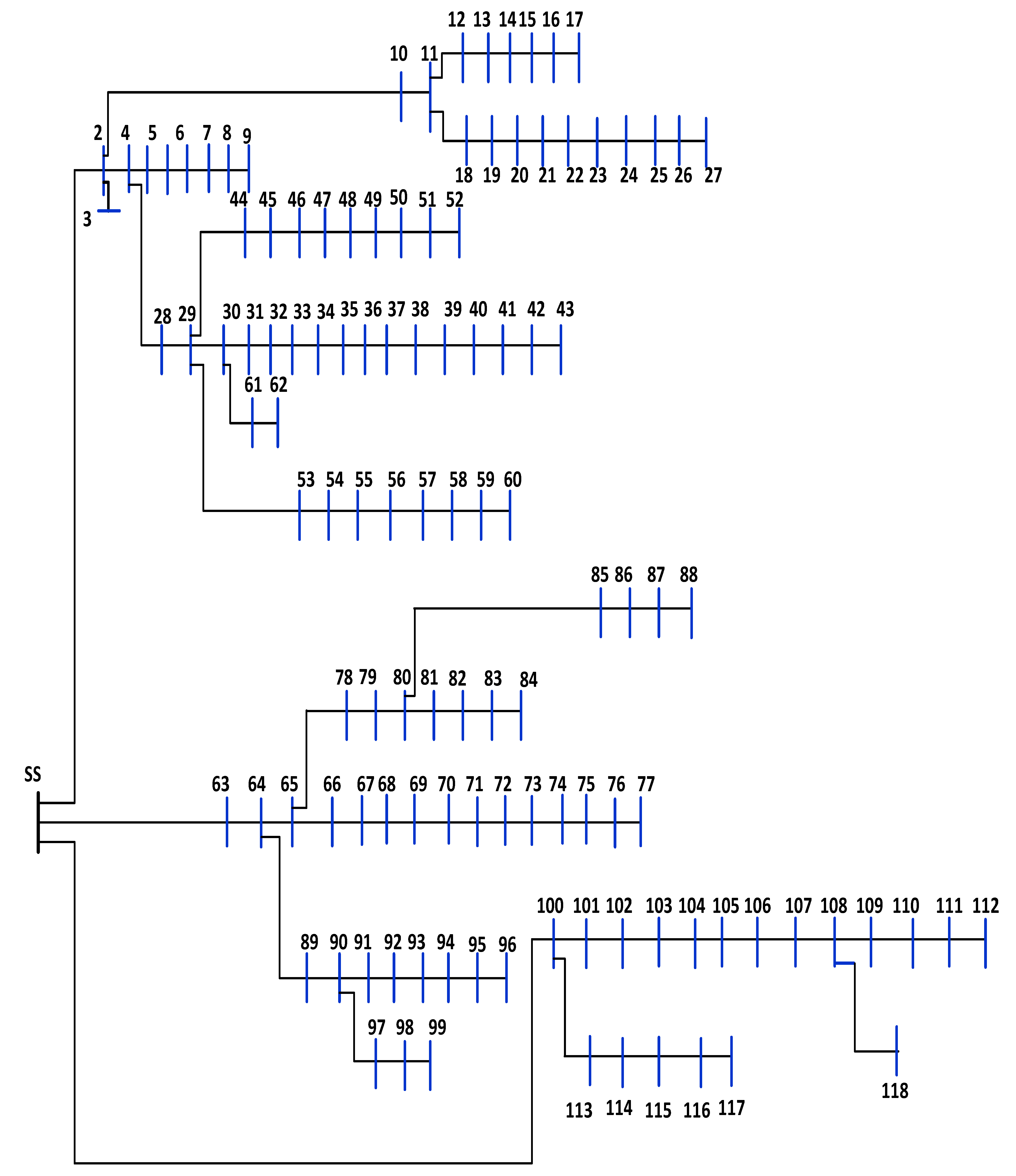
5.1.1. Case Study 1: IEEE 118-Bus System

MRFO was utilized to determine the optimal RER placements and ratings in the IEEE 118-bus system shown in Figure 5. Without any penetration of RERs, the expected cost, emissions, voltage deviations, and the expected voltage stability index were 1633.5 USD/h, 34,842,000 kg/MWh, 4.2157 p.u., and 101.4379 p.u., respectively. In the case of optimal insertion of WT- and solar PV-based DGs, these calculations became 975.7504 USD/h, 13,029,000 kg/MWh, 2.9794 p.u., and 106.5046 p.u., respectively. In other words, these values are enhanced by 40.27%, 62.6%, 29.33%, and 4.76%, respectively. The optimal sites of the PV units and the WT-based DGs were buses 72 and 64, respectively. These DGs should be of the following optimum sizes: 2589.53 kW and 20,029.39 kW.

Table 6. The IEEE 118-bus system simulation results.

Scenario	$\mathit{\pi }\text{\_}\mathit{s}$	Loading %	${\mathit{P}}_{\mathit{w}} \left(\mathbf{k}\mathbf{W}\right)$	${\mathit{P}}_{\mathit{s}} \left(\mathbf{k}\mathbf{W}\right)$	$\mathit{E}\mathit{T}\mathit{C}\mathit{o}\mathit{s}\mathit{t} \left(\mathbf{U}\mathbf{S}\mathbf{D}/\mathbf{h}\right)$	$\mathit{E}\mathit{T}\mathit{E}\mathit{m}\mathit{i}\mathit{s}\mathit{s}\mathit{i}\mathit{o}\mathit{n}$ (kg/MWh)	$\mathit{E}\mathit{T}\mathit{V}\mathit{D} \left(\mathbf{p}.\mathbf{u}.\right)$	$\mathit{E}\mathit{T}\mathit{V}\mathit{S}\mathit{I} \left(\mathbf{p}.\mathbf{u}.\right)$
$\mathrm{S}1$	0.0010	82.1	4180	2136.9	1.6	26,800	0.0033	0.1045
$\mathrm{S}2$	0.0030	85.9	7765	1724.5	4.2	66,600	0.0096	0.3156
$\mathrm{S}3$	0.1050	72.8	9696	806	107.5	1,465,700	0.301	11.1894
$\mathrm{S}4$	0.0060	58.2	2460	139.2	8.3	138,600	0.0204	0.6253
$\mathrm{S}5$	0.0040	75.4	6227	1927.5	5.1	79,400	0.0118	0.424
$\mathrm{S}6$	0.1040	68.4	7290	522.6	119.9	1,798,900	0.317	10.9873
$\mathrm{S}7$	0.0110	73.8	2036	1516.4	18.1	313,900	0.0387	1.1417
$\mathrm{S}8$	0.0470	63.7	11,735	933.8	29.9	248,000	0.1215	5.112
$\mathrm{S}9$	0.0330	78.1	8056	1052.9	41.6	635,600	0.1027	3.4809
$\mathrm{S}10$	0.0010	64.5	4179	2356	1.2	17,900	0.0027	0.1069
$\mathrm{S}11$	0.0530	66.1	16,287	649.1	17.9	0	0.1559	5.8439
$\mathrm{S}12$	0.1210	72.9	8878	345.6	137.5	2,014,500	0.3737	12.7797
$\mathrm{S}13$	0.0160	64.4	8890	1307.4	13.7	167,600	0.0405	1.7251
$\mathrm{S}14$	0.0100	65.4	11,281	1179.9	6.9	64,500	0.0255	1.0866
$\mathrm{S}15$	0.4850	72.1	11,201	0	462.2	5,990,800	1.455	51.5818
Summation	1				975.7503	13,028,800	2.9793	106.5047

shows the PV unit and WT-based DG output powers, as well as the expected values for each scenario. It can be seen that the numbers changed in each scenario due to the differences in the RER output power and load demand. Furthermore, it can be observed that scenario number 15 had the highest projected expenses, expected emissions, and predicted voltage variation. This was due to the out power of the solar PV being 0 kW. As a result, the majority of the required power would be provided by the grid, causing these values to rise. Cost, emissions, VDs, and the VSIs for each scenario with and without the integration of the RERs are shown in Figure 8, Figure 9, Figure 10 and Figure 11, respectively. According to these figures, the cost, emissions, and VDs were reduced significantly in each scenario with the inclusion of RERs, while the VSI at each scenario was enhanced considerably. Figure 12 and Figure 13 depict the voltage profiles of the IEEE 118-bus system for each situation. It is obvious that the insertion of RERs can improve the voltage profile for each scenario.

Table 7. The statistical results in the IEEE 118-bus system with the use of several optimizers.

Optimizer	Best Values	Average Values	Worst Values	SD
MRFO	0.6820	0.7087	0.7655	0.0253
PSO	0.7097	0.7547	0.8333	0.0374
ALO	0.7323	0.7985	0.8625	0.0358
WOA	0.7745	0.8132	0.8903	0.0175
SCA	0.6942	0.7351	0.7905	0.0306

lists the statistical findings of the objective function calculated using several optimization techniques, namely, WOA (whale optimization algorithm) [30], PSO (particle swarm optimization) [31], ALO (ant lion optimizer) [32], and SCA (sine cosine algorithm) [33]. It can be observed that the MRFO surpasses other methods for solving this problem.

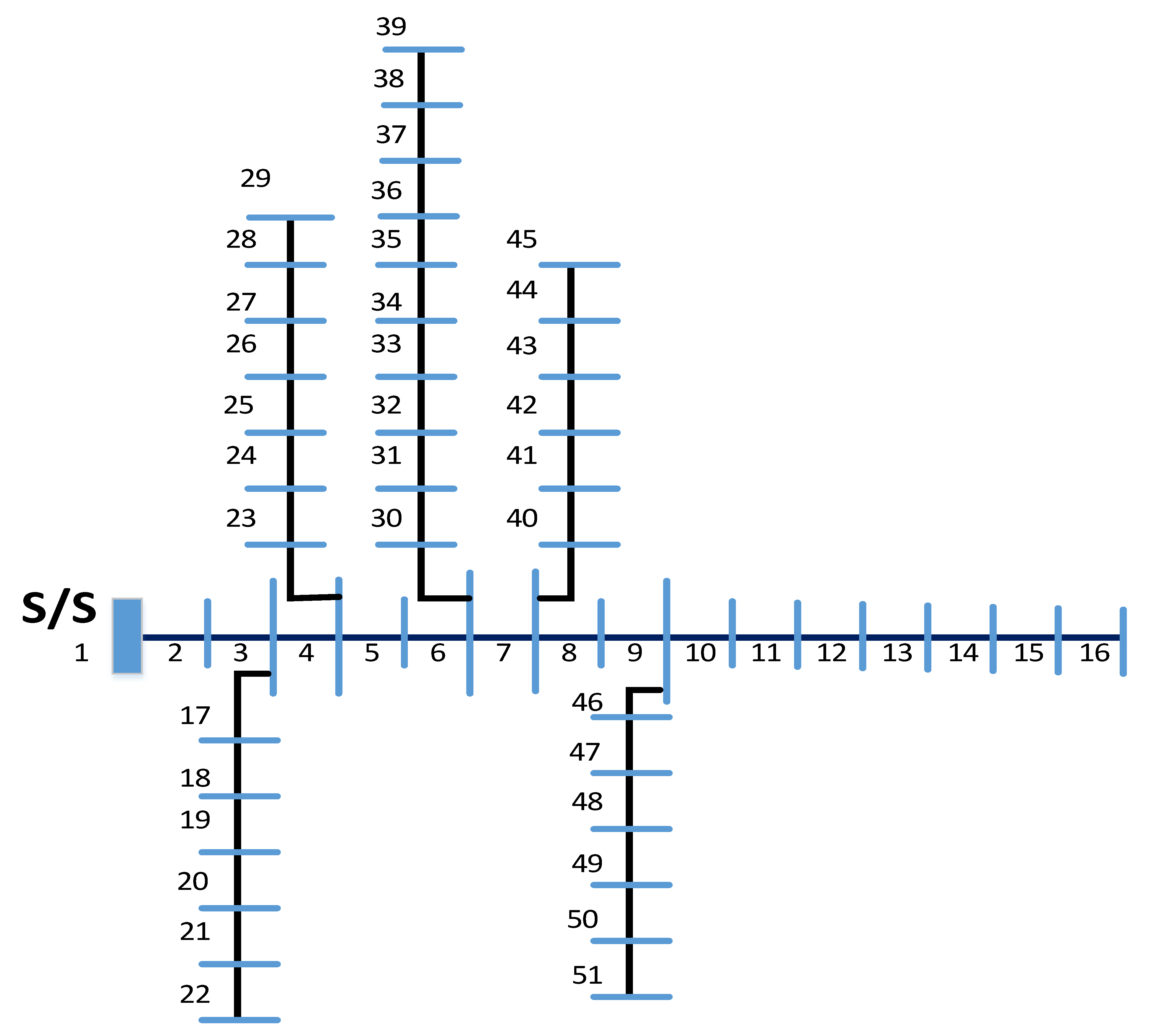
5.1.2. Case Study 2: Rural 51-Bus System

In this case study, MRFO was employed to identify the optimal RER locations and ratings in the 51-bus system shown in Figure 6. Without RERs, the expected cost, emissions, voltage deviation, and the expected voltage stability index were 176.0419 USD/h, 3,754,900 kg/MWh, 2.1514 p.u., and 41.9992 p.u., respectively. In the case of the optimal insertion of WT and solar PV-based DGs, these respective values improved to 113.4299 USD/h, 1,504,600 kg/MWh, 0.6678 p.u., and 47.6629 p.u. with a percentage improvement of 35.57%, 59.92%, 68.95%, and 11.88%, in each respective parameter. The optimal sites of the PV units and the WT were buses 43 and 9, respectively. The optimum sizes of these DGs were found to be 574.58 kW and 1884.61 kW, respectively.

Table 8. The 51-bus system simulation results.

Scenario	$\mathit{\pi }\text{\_}\mathit{s}$	Loading %	${\mathit{P}}_{\mathit{w}} \left(\mathbf{k}\mathbf{W}\right)$	${\mathit{P}}_{\mathit{s}} \left(\mathbf{k}\mathbf{W}\right)$	$\mathit{E}\mathit{T}\mathit{C}\mathit{o}\mathit{s}\mathit{t} \left(\mathbf{U}\mathbf{S}\mathbf{D}/\mathbf{h}\right)$	$\mathit{E}\mathit{T}\mathit{E}\mathit{m}\mathit{i}\mathit{s}\mathit{s}\mathit{i}\mathit{o}\mathit{n}$ (kg/MWh)	$\mathit{E}\mathit{T}\mathit{V}\mathit{D} \left(\mathbf{p}.\mathbf{u}.\right)$	$\mathit{E}\mathit{T}\mathit{V}\mathit{S}\mathit{I} \left(\mathbf{p}.\mathbf{u}.\right)$
$\mathrm{S}1$	0.0010	82.1	393.4	474.4	0.1574	2460	0.0013	0.0451
$\mathrm{S}2$	0.0030	85.8	730.8	82.8	0.4317	6380	0.0028	0.1393
$\mathrm{S}3$	0.1050	72.8	912.5	78.9	11.9328	157,040	0.0653	4.9954
$\mathrm{S}4$	0.0060	58.2	231.5	0.9057	0.9118	14,940	0.0092	0.2651
$\mathrm{S}5$	0.0040	75.4	586.1	27.9	0.5107	7190	0.0037	0.1857
$\mathrm{S}6$	0.1040	68.4	686.1	16.1	13.3313	194,260	0.0973	4.8225
$\mathrm{S}7$	0.0110	73.8	191.6	36.7	1.8425	30,250	0.0174	0.4842
$\mathrm{S}8$	0.0470	63.7	1104.4	07.3	3.4467	27,710	0.0163	2.3186
$\mathrm{S}9$	0.0330	78.1	758.2	33.8	4.4574	65,000	0.0292	1.5367
$\mathrm{S}10$	0.0010	64.5	393.3	23.1	0.1111	1460	0.001	0.0463
$\mathrm{S}11$	0.0530	66.1	1532.8	44.1	2.6	90	0.0277	2.7232
$\mathrm{S}12$	0.1210	72.9	835.5	6.7	15.6	226,480	0.1	5.661
$\mathrm{S}13$	0.0160	64.4	836.7	90.3	1.5	15,890	0.008	0.7691
$\mathrm{S}14$	0.0100	65.4	1061.7	261.9	0.7632	6480	0.0037	0.4917
$\mathrm{S}15$	0.4850	72.1	1054.2	0	55.8	748,990	0.285	23.1788
Summation	1				113.4299	1,504,620	0.6679	47.6627

shows the PV and WT output powers, as well as the expected values for each studied scenario. Similar to the above case study, the values in Table 8 changed for each scenario due to the changes in RER generation and the variation of the load demand. It can be seen that the highest values of the expected cost, emissions, and voltage deviation occurred in scenario number 15, where no solar-based power is generated. The values of the cost, emissions, VDs and the VSIs for each scenario with and without the integration of RERs are shown in Figure 14, Figure 15, Figure 16 and Figure 17, respectively. These figures reveal that the cost, emissions, and VDs were reduced significantly in each scenario with the inclusion of RERs, along with a considerable enhancement in the VSI. In addition, Figure 18 and Figure 19 depict the voltage profiles of the 51-bus system for each situation. It is obvious that the integration of RERs at a proper location and with an optimum sizing can improve the voltage profile at each bus for all scenarios.

Table 9. The statistical results in the rural 51-bus system with the use of several optimizers.

Optimizer	Best Values	Average Values	Worst Values	SD Values
MRFO	0.6226	0.6367	0.6562	0.0093
PSO	0.6478	0.7367	0.8431	0.0545
ALO	0.6318	0.7220	0.8824	0.0534
WOA	0.6530	0.7138	0.8002	0.0412
SCA	0.6418	0.6686	0.7018	0.0178

shows the statistical results of the objective function calculated using different optimization algorithms. Results in Table 9 attest to the superiority of the proposed MRFO technique over all other optimization methods, namely, PSO, WOA, SCA, and ALO.

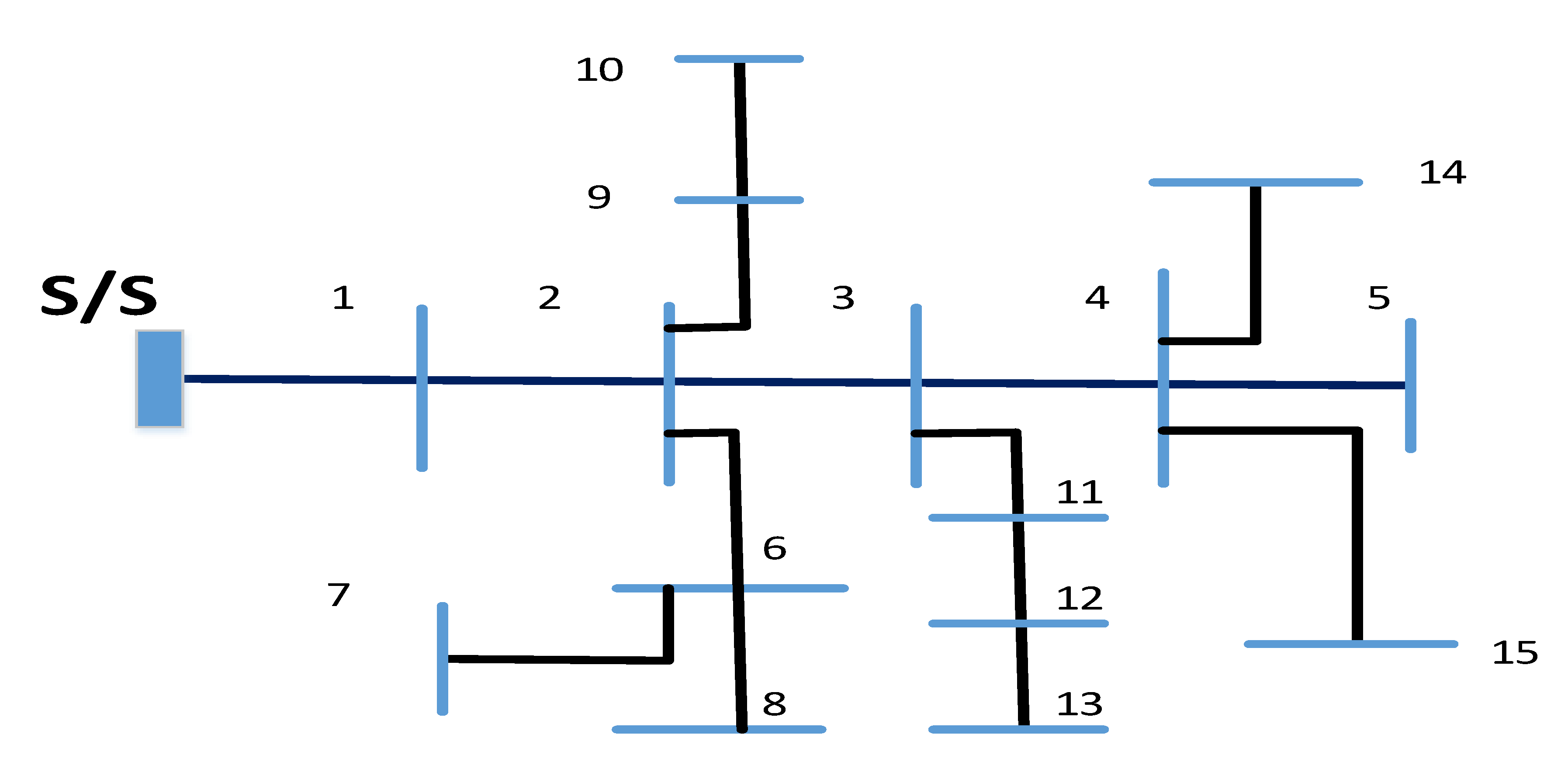
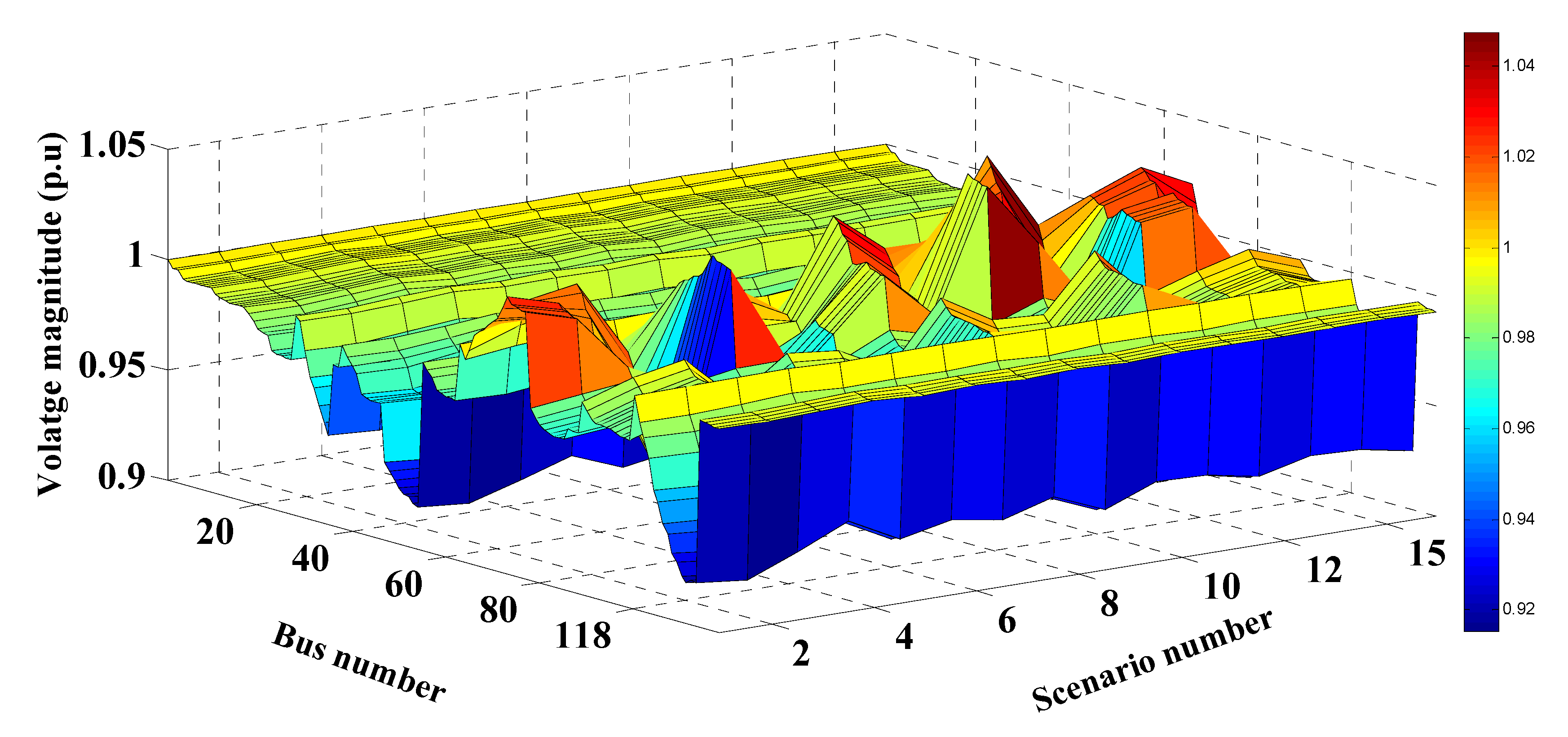
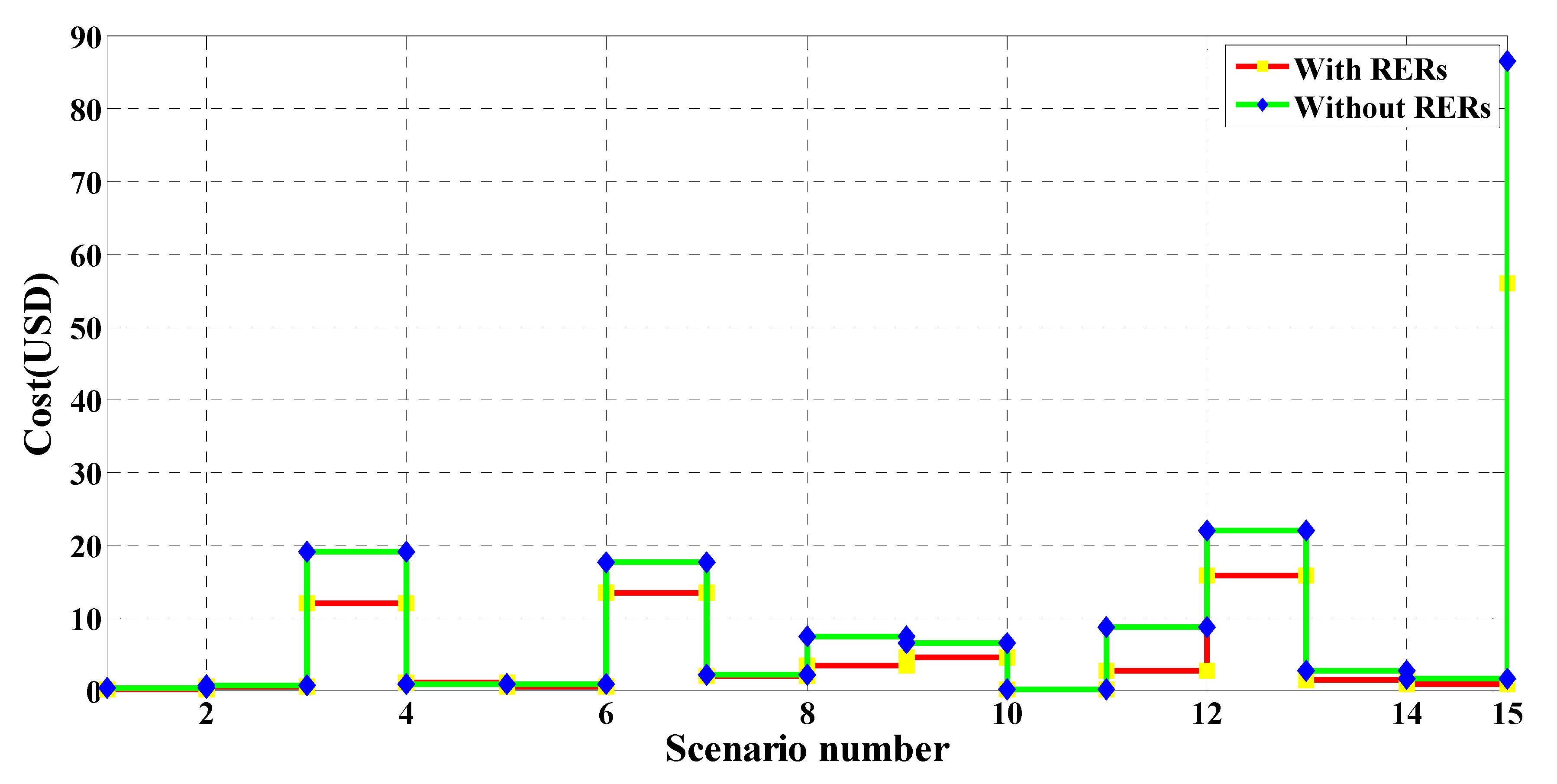
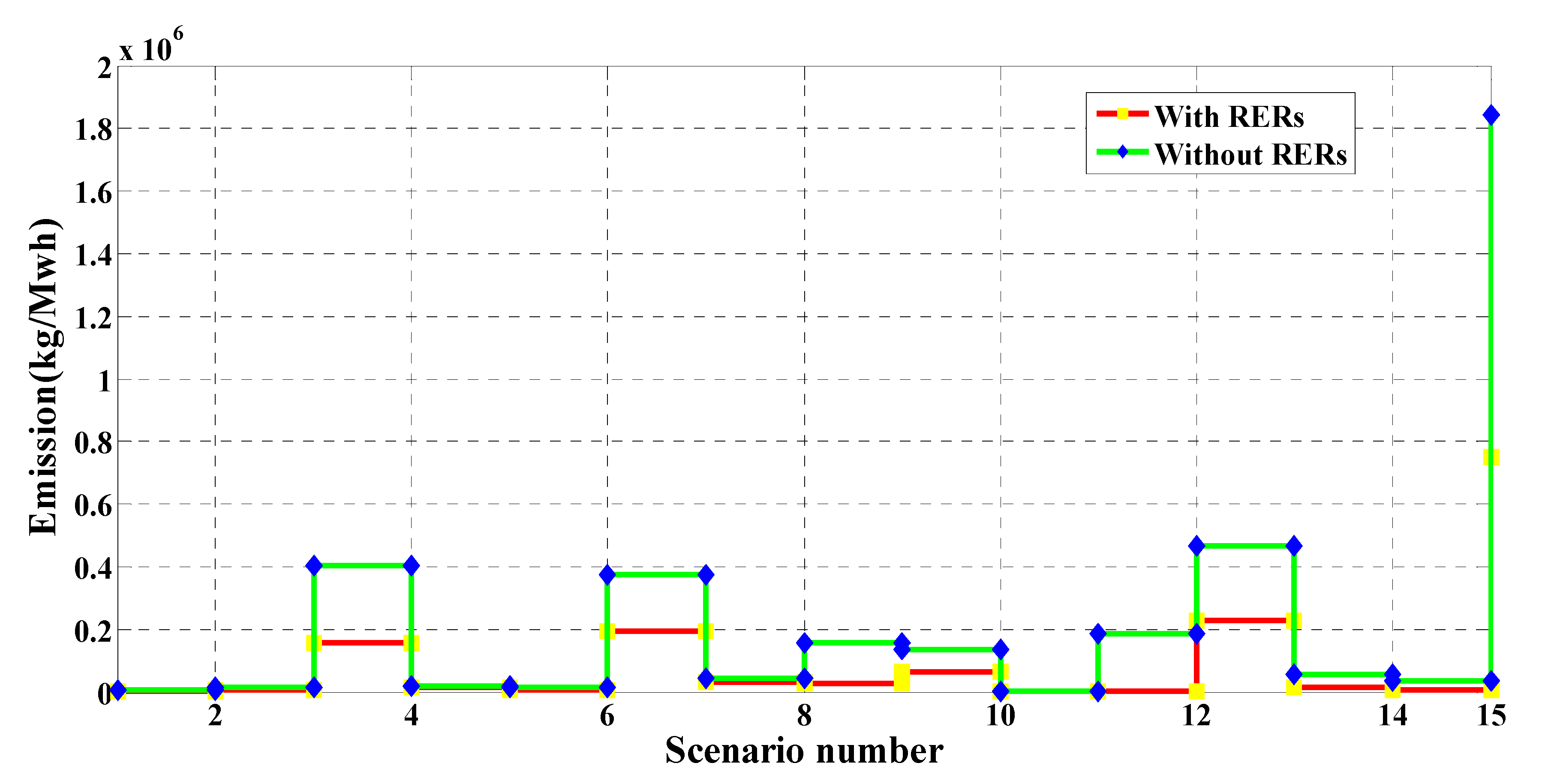
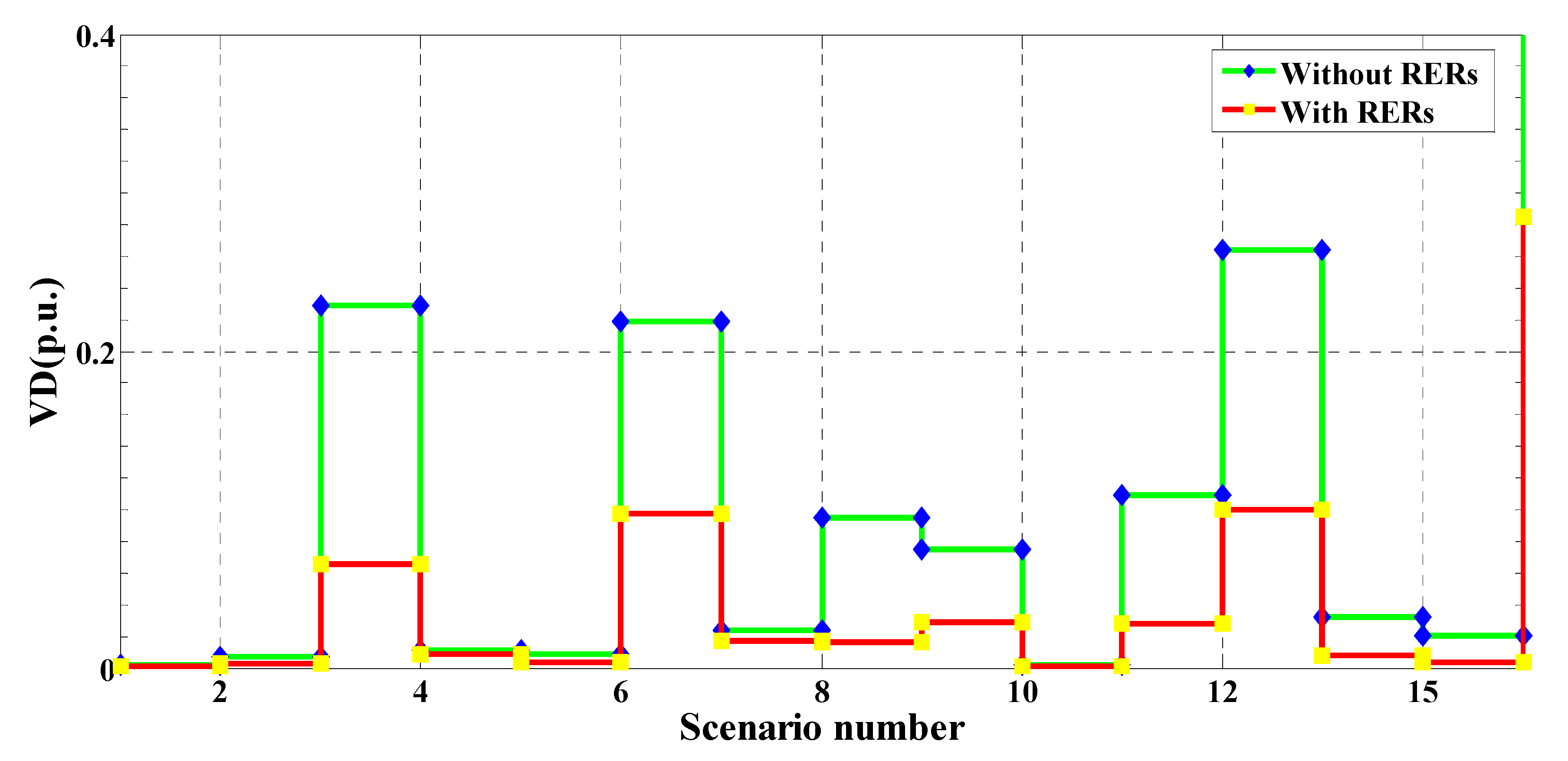
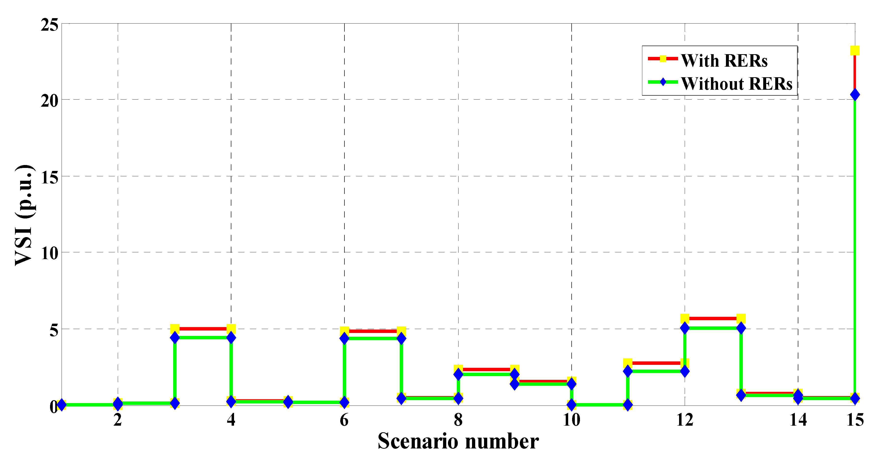
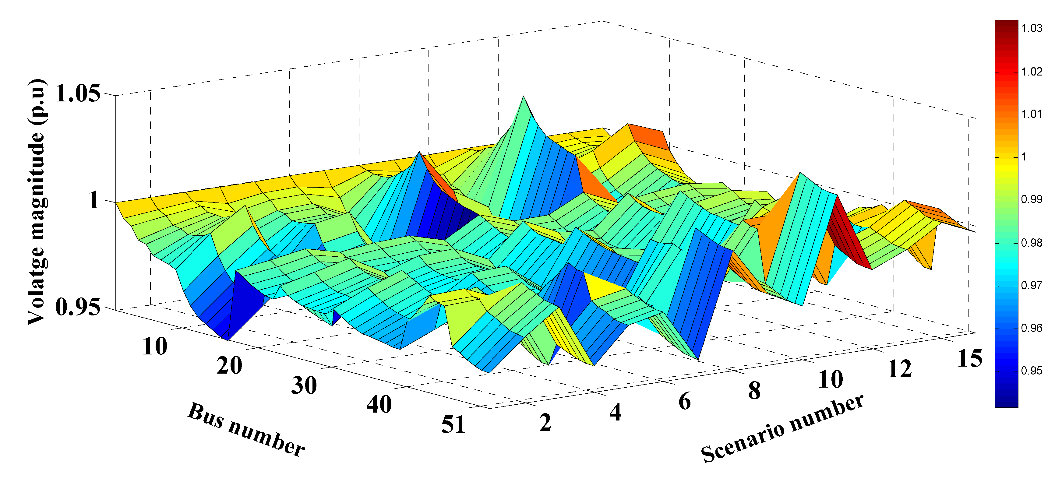
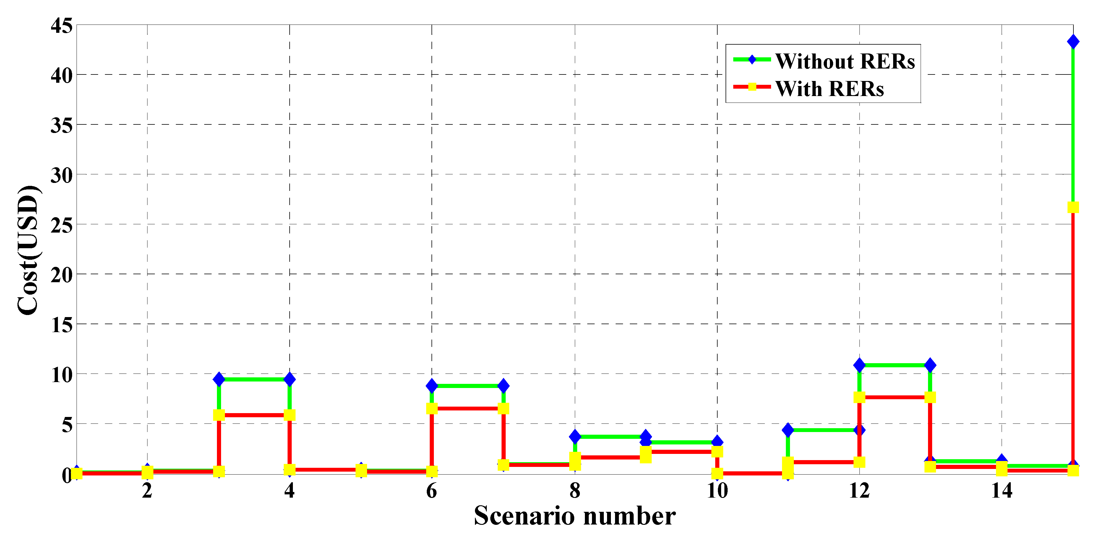
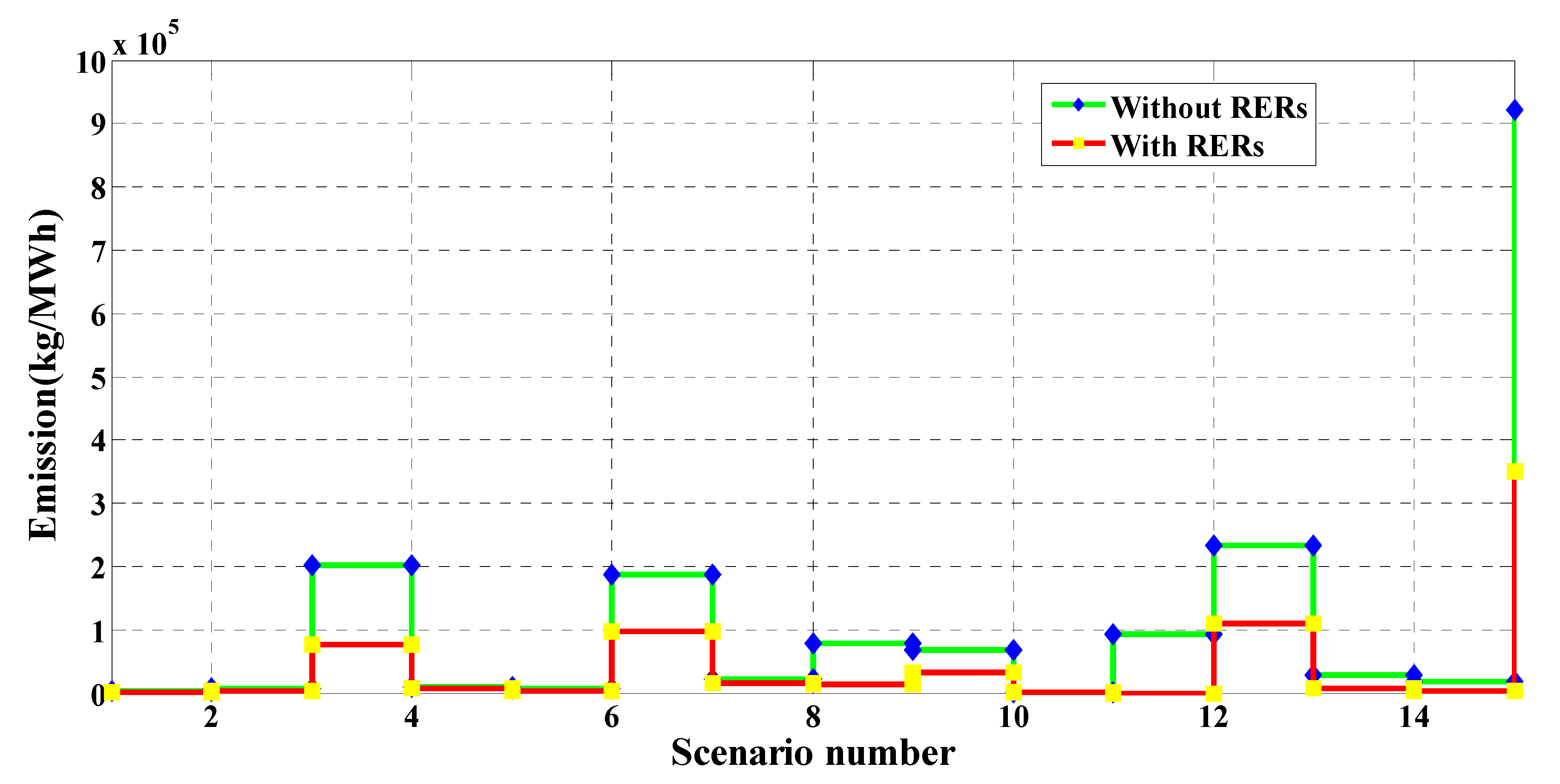
5.1.3. Case Study 3: Small 15-Bus System

In this case study, MRFO was employed to identify the optimal RER locations and ratings within the 15-bus system shown in Figure 7. Without RERs, the expected cost, emissions, voltage deviation, and the expected voltage stability index were 88.1005 USD/h, 1,879,200 kg/MWh, 0.5313 p.u., and 12.0005 p.u., respectively. In the case of the optimal insertion of WT and solar PV-based DGs, these respective values improved to 54.8523 USD/h, 724,180 kg/MWh, 0.2211 p.u., and 13.1670 p.u., with a percentage improvement of 37.74%, 61.46%, 58.39%, and 8.86%, in each respective parameter. The optimal sites of the PV units and the WT were buses 14 and 11, respectively. The optimum sizes of these DGs are found to be 249 kW and 977 kW, respectively.

Table 10. The 15-bus system simulation results.

Scenario	$\mathit{\pi }\text{\_}\mathit{s}$	Loading %	${\mathit{P}}_{\mathit{w}}\left(\mathbf{k}\mathbf{W}\right)$	${\mathit{P}}_{\mathit{s}}\left(\mathbf{k}\mathbf{W}\right)$	$\mathit{E}\mathit{T}\mathit{C}\mathit{o}\mathit{s}\mathit{t} \left(\mathbf{U}\mathbf{S}\mathbf{D}/\mathbf{h}\right)$	$\mathit{E}\mathit{T}\mathit{E}\mathit{m}\mathit{i}\mathit{s}\mathit{s}\mathit{i}\mathit{o}\mathit{n}$ (kg/MWh)	$\mathit{E}\mathit{T}\mathit{V}\mathit{D} \left(\mathbf{p}.\mathbf{u}.\right)$	$\mathit{E}\mathit{T}\mathit{V}\mathit{S}\mathit{I} \left(\mathbf{p}.\mathbf{u}.\right)$
$\mathrm{S}1$	0.0010	82.1	203.9	205.4	0.0801	1280	0.0004	0.0125
$\mathrm{S}2$	0.0030	85.9	378.8	165.8	0.2165	3250	0.0009	0.0386
$\mathrm{S}3$	0.1050	72.8	472.9	77.5	5.852	77,200	0.0237	1.3783
$\mathrm{S}4$	0.0060	58.2	119.9	13.4	0.4542	7500	0.0025	0.0746
$\mathrm{S}5$	0.0040	75.4	303.8	185.3	0.2589	3740	0.0012	0.0513
$\mathrm{S}6$	0.1040	68.4	355.6	50.3	6.5761	96,310	0.0301	1.34
$\mathrm{S}7$	0.0110	73.8	99.3	145.8	0.9357	15,610	0.0048	0.1358
$\mathrm{S}8$	0.0470	63.7	572.4	89.8	1.6609	13,010	0.0067	0.6332
$\mathrm{S}9$	0.0330	78.1	392.9	101.2	2.2128	32,570	0.0093	0.426
$\mathrm{S}10$	0.0010	64.5	203.9	226.5	0.0574	790	0.0003	0.0128
$\mathrm{S}11$	0.0530	66.1	794.5	62.4	1.148	0	0.0063	0.7375
$\mathrm{S}12$	0.1210	72.9	433.1	33.3	7.638	110,400	0.0317	1.5715
$\mathrm{S}13$	0.0160	64.4	433.6	125.7	0.7221	8070	0.0033	0.211
$\mathrm{S}14$	0.0100	65.4	550.3	113.4	0.3721	3150	0.0015	0.1343
$\mathrm{S}15$	0.4850	72.1	546.4	0	26.6676	351,300	0.0983	6.4095
Summation	1				54.8524	724,180	0.2211	13.1669

shows the PV and WT output powers, as well as the expected values for each studied scenario. Similar to the above case studies, the values in Table 10 changed for each scenario due to the changes in RER generation and the variation of the load demand. It can be seen that the highest values of the expected cost, emissions, and voltage deviation occurred in scenario number 15, where no solar-based power is generated. The values of the cost, emissions, VDs, and the VSIs for each scenario with and without the integration of RERs are shown in Figure 20, Figure 21, Figure 22 and Figure 23, respectively. These figures reveal that the cost, emissions, and VDs were reduced significantly for each scenario with the inclusion of RERs, along with a considerable enhancement in the VSI. In addition, Figure 24 and Figure 25 depict the voltage profiles of the 15-bus system for each situation. It is obvious that the integration of RERs at a proper location and with an optimum sizing can improve the voltage profile at each bus for all scenarios.

Table 11. The statistical results in the 15-bus system with the use of several optimizers.

Optimizer	Average Values	Best Values	Worst Values	SD Values
MRFO	0.6345	0.6303	0.6426	0.0030
PSO	0.7201	0.6482	0.9301	0.0676
ALO	0.6832	0.6367	0.7515	0.0357
WOA	0.6695	0.6339	0.7917	0.0444
SCA	0.6485	0.6355	0.6665	0.0107

tabulates the statistical results of the objective function calculated using different optimization algorithms. Results in Table 11 attest to the superiority of the proposed MRFO technique over all other optimization methods, namely, PSO, WOA, SCA, and ALO.

5.2. Discussions

From the results of the above three studied systems, the key conclusion points can be summarized as follows:

• The MFRO is an efficient algorithm for solving the allocation problem of the DGs in distribution systems that comprise uncertainty of the load demand and power generation from intermittent renewable energy sources.
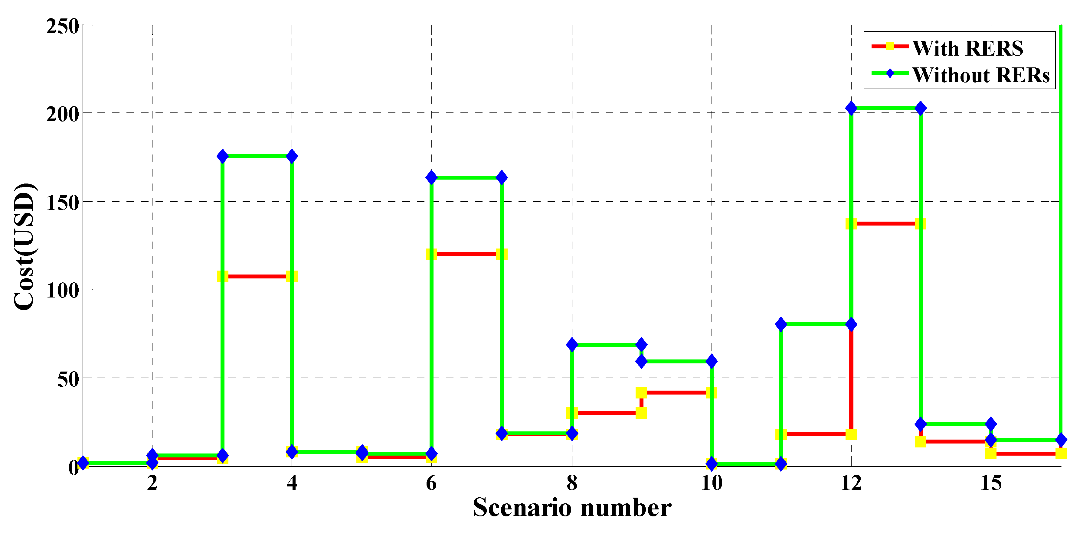
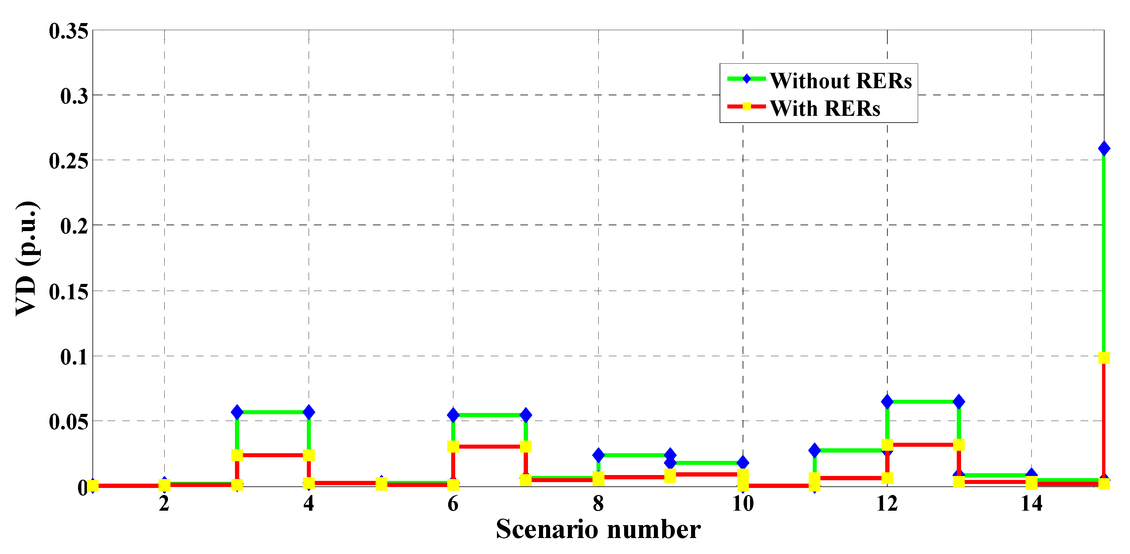
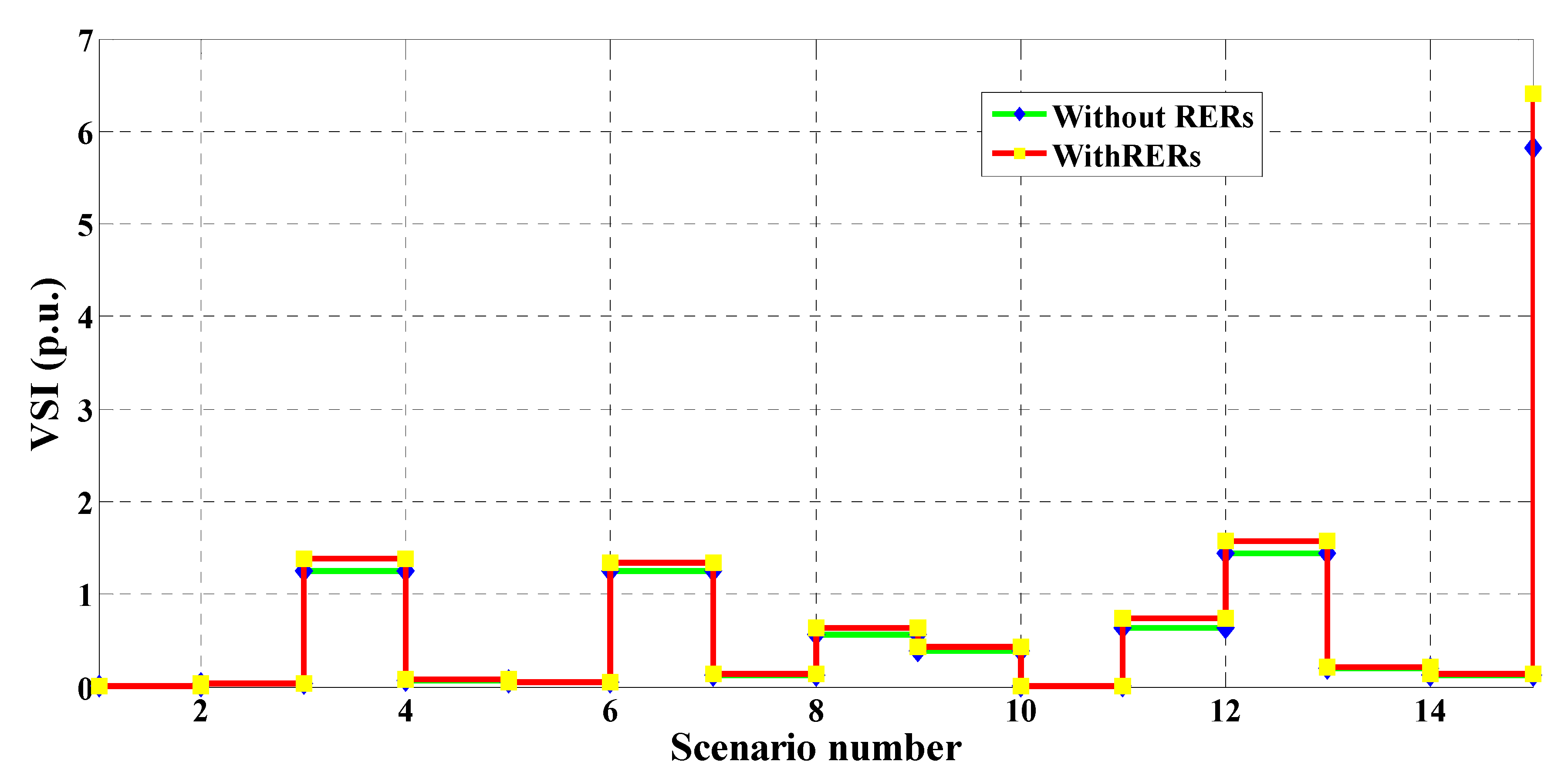
• The cost, emissions, and VDs are significantly reduced with the inclusion of RERs, while the VSI is significantly enhanced.
• The Monte Carlo simulation approach and backward reduction algorithm were successfully applied for modeling electrical system uncertainty.

6. Conclusions

This paper introduced the manta ray foraging optimizer (MRFO) as an efficient optimizer for identifying the optimal sizing and location of renewable-based DGs in RDN. A multi-objective function comprising total cost, emission, voltage deviation, and system stability was proposed and solved using the MRFO with consideration of the uncertainty of solar irradiance, load demand, and wind speed. The lognormal and normal Weibull PDFs were employed to emulate these uncertainties. Furthermore, Monte Carlo simulation was used to generate a set of scenarios (1000 scenario), which was reduced to 15 dominant scenarios using the backward reduction method. The robustness of the proposed optimization method was assessed through its applications on three radial distribution networks: IEEE 118-bus, rural 51-bus, and IEEE 15-bus distribution systems. Results show that, when considering the uncertainties and optimal insertion of solar PV- and wind turbine-based DGs, the expected cost, emission, voltage deviation, and the voltage stability index were improved by 40.27%, 62.6%, 29.33%, and 4.76%, respectively, for the IEEE 118-bus case study. For the 51-bus case study, if the uncertainties were taken into account, and the solar PV- and WT-based DGs were optimally allocated, these values were improved by 35.57%, 59.92%, 68.95%, and 11.88%, respectively. For the 15-bus case study, if the uncertainties were taken into account, and the solar PV- and WT-based DGs were optimally allocated, these values were improved by 37.74%, 61.46%, 58.39%, and 8.86%, respectively. Compared to other optimization techniques (PSO, ALO, WOA, and SCA), the results reveal the superiority of the proposed algorithm in solving the allocation and sizing problem of the renewable-based DGs under deterministic and probabilistic states.

References

1. Prakash, P. Optimal DG Allocation Using Particle Swarm Optimization. In Proceedings of the 2021 International Conference on Artificial Intelligence and Smart Systems (ICAIS), Coimbatore, India, 25–27 March 2021; pp. 940–944. [Google Scholar]
2. Lakshmi, G.S.; Rubanenko, O.; Divya, G.; Lavanya, V. Distribution Energy Generation using Renewable Energy Sources. In Proceedings of the 2020 IEEE India Council International Subsections Conference (INDISCON), Visakhapatnam, India, 3–4 October 2020; pp. 108–113. [Google Scholar]
3. Biswas, P.P.; Suganthan, P.N.; Mallipeddi, R.; Amaratunga, G.A.J. Optimal reactive power dispatch with uncertainties in load demand and renewable energy sources adopting scenario-based approach. Appl. Soft Comput. J. 2019, 75, 616–632. [Google Scholar] [CrossRef]
4. Karunarathne, E.; Pasupuleti, J.; Ekanayake, J.; Almeida, D. Optimal placement and sizing of DGs in distribution networks using MLPSO algorithm. Energies 2020, 13, 6185. [Google Scholar] [CrossRef]
5. Ramadan, A.; Ebeed, M.; Kamel, S.; Abdelaziz, A.Y.; Alhelou, H.H. Scenario-Based Stochastic Framework for Optimal Planning of Distribution Systems Including Renewable-Based DG Units. Sustainability 2021, 13, 3566. [Google Scholar] [CrossRef]
6. Devineni, G.K.; Ganesh, A.; Rao, D.N.M.; Saravanan, S. Optimal Sizing and Placement of DGs to Reduce the Fuel Cost and T & D Losses by using GA & PSO optimization Algorithms. In Proceedings of the 2021 International Conference on Sustainable Energy and Future Electric Transportation (SEFET), Hyderabad, India, 21–23 January 2021; pp. 1–6. [Google Scholar]
7. Zellagui, M.; Belbachir, N.; El-Bayeh, C.Z. Optimal Allocation of RDG in Distribution System Considering the Seasonal Uncertainties of Load Demand and Solar-Wind Generation Systems. In Proceedings of the IEEE EUROCON 2021—19th International Conference on Smart Technologies, Lviv, Ukraine, 6–8 July 2021; pp. 471–477. [Google Scholar]
8. Elkadeem, M.R.; Elaziz, M.A.; Ullah, Z.; Wang, S.; Sharshir, S.W. Optimal planning of renewable energy-integrated distribution system considering uncertainties. IEEE Access 2019, 7, 164887–164907. [Google Scholar] [CrossRef]
9. Zellagui, M.; Lasmari, A.; Settoul, S.; El-Sehiemy, R.A.; El-Bayeh, C.Z.; Chenni, R. Simultaneous allocation of photovoltaic DG and DSTATCOM for techno-economic and environmental benefits in electrical distribution systems at different loading conditions using novel hybrid optimization algorithms. Int. Trans. Electr. Energy Syst. 2021, 31, e12992. [Google Scholar] [CrossRef]
10. Venkatesan, C.; Kannadasan, R.; Alsharif, M.H.; Kim, M.-K.; Nebhen, J. A Novel Multiobjective Hybrid Technique for Siting and Sizing of Distributed Generation and Capacitor Banks in Radial Distribution Systems. Sustainability 2021, 13, 3308. [Google Scholar] [CrossRef]
11. Hemeida, M.G.; Alkhalaf, S.; Senjyu, T.; Ibrahim, A.; Ahmed, M.; Bahaa-Eldin, A.M. Optimal probabilistic location of DGs using Monte Carlo simulation based different bio-inspired algorithms. Ain Shams Eng. J. 2021, 12, 2735–2762. [Google Scholar] [CrossRef]
12. Rathore, A.; Patidar, N. Optimal sizing and allocation of renewable based distribution generation with gravity energy storage considering stochastic nature using particle swarm optimization in radial distribution network. J. Energy Storage 2021, 35, 102282. [Google Scholar] [CrossRef]
13. el Sehiemy, R.A.; Selim, F.; Bentouati, B.; Abido, M. A novel multi-objective hybrid particle swarm and salp optimization algorithm for technical-economical-environmental operation in power systems. Energy 2020, 193, 116817. [Google Scholar] [CrossRef]
14. Ahmed, D.; Ebeed, M.; Ali, A.; Alghamdi, A.S.; Kamel, S. Multi-objective energy management of a micro-grid considering stochastic nature of load and renewable energy resources. Electronics 2021, 10, 403. [Google Scholar] [CrossRef]
15. Rao, B.N.; Abhyankar, A.; Senroy, N. Optimal placement of distributed generator using monte carlo simulation. In Proceedings of the 2014 Eighteenth National Power Systems Conference (NPSC), Guwahati, India, 18–20 December 2014; pp. 1–6. [Google Scholar]
16. Thokar, R.A.; Gupta, N.; Niazi, K.; Swarnkar, A.; Sharma, S.; Meena, K. Optimal integration and management of solar generation and battery storage system in distribution systems under uncertain environment. Int. J. Renew. Energy Res. 2020, 10, 11–12. [Google Scholar]
17. Biswal, S.R.; Shankar, G. Simultaneous optimal allocation and sizing of DGs and capacitors in radial distribution systems using SPEA2 considering load uncertainty. IET Gener. Transm. Distrib. 2020, 14, 494–505. [Google Scholar] [CrossRef]
18. Elattar, E.E.; Shaheen, A.M.; El-Sayed, A.M.; El-Sehiemy, R.A.; Ginidi, A.R. Optimal operation of automated distribution networks based-MRFO algorithm. IEEE Access 2021, 9, 19586–19601. [Google Scholar] [CrossRef]
19. Zhao, W.; Zhang, Z.; Wang, L. Manta ray foraging optimization: An effective bio-inspired optimizer for engineering applications. Eng. Appl. Artif. Intell. 2020, 87, 103300. [Google Scholar] [CrossRef]
20. El-Ela, A.A.A.; El-Sehiemy, R.A.; Abbas, A.S. Optimal placement and sizing of distributed generation and capacitor banks in distribution systems using water cycle algorithm. IEEE Syst. J. 2018, 12, 3629–3636. [Google Scholar] [CrossRef]
21. Hassan, M.H.; Kamel, S.; El-Dabah, M.A.; Khurshaid, T.; Domínguez-García, J.L. Optimal reactive power dispatch with time-varying demand and renewable energy uncertainty using Rao-3 algorithm. IEEE Access 2021, 9, 23264–23283. [Google Scholar] [CrossRef]
22. Mohseni-Bonab, S.M.; Rabiee, A. Optimal reactive power dispatch: A review, and a new stochastic voltage stability constrained multi-objective model at the presence of uncertain wind power generation. IET Gener. Transm. Distrib. 2017, 11, 815–829. [Google Scholar] [CrossRef]
23. Biswas, P.P.; Suganthan, P.N.; Amaratunga, G.A.J. Optimal power flow solutions incorporating stochastic wind and solar power. Energy Convers. Manag. 2017, 148, 1194–1207. [Google Scholar] [CrossRef]
24. Soroudi, A.; Aien, M.; Ehsan, M. A probabilistic modeling of photo voltaic modules and wind power generation impact on distribution networks. IEEE Syst. J. 2012, 6, 254–259. [Google Scholar] [CrossRef] [Green Version]
25. Hemeida, M.G.; Ibrahim, A.A.; Mohamed, A.-A.A.; Alkhalaf, S.; El-Dine, A.M.B. Optimal allocation of distributed generators DG based Manta Ray Foraging Optimization algorithm (MRFO). Ain Shams Eng. J. 2021, 12, 609–619. [Google Scholar] [CrossRef]
26. Vahid, M.Z.; Ali, Z.M.; Najmi, E.S.; Ahmadi, A.; Gandoman, F.H.; Aleem, S.H. Optimal Allocation and Planning of Distributed Power Generation Resources in a Smart Distribution Network Using the Manta Ray Foraging Optimization Algorithm. Energies 2021, 14, 4856. [Google Scholar] [CrossRef]
27. Eid, A.; Abdelaziz, A.Y.; Dardeer, M. Energy Loss Reduction of Distribution Systems Equipped with Multiple Distributed Generations Considering Uncertainty using Manta-Ray Foraging Optimization. Int. J. Renew. Energy Dev. 2021, 10, 779–787. [Google Scholar] [CrossRef]
28. Ramadan, A.; Ebeed, M.; Kamel, S.; Nasrat, L. Optimal allocation of renewable energy resources considering uncertainty in load demand and generation. In Proceedings of the 2019 IEEE Conference on Power Electronics and Renewable Energy (CPERE), Aswan, Egypt, 23–25 October 2019; pp. 124–128. [Google Scholar]
29. Gampa, S.R.; Das, D. Optimum placement and sizing of DGs considering average hourly variations of load. Int. J. Electr. Power Energy Syst. 2015, 66, 25–40. [Google Scholar] [CrossRef]
30. Ang, S.; Leeton, U. Optimal placement and size of distributed generation in radial distribution system using whale optimization algorithm. Suranaree J. Sci. Technol. 2019, 26, 1–12. [Google Scholar]
31. Bhumkittipich, K.; Phuangpornpitak, W. Optimal placement and sizing of distributed generation for power loss reduction using particle swarm optimization. Energy Procedia 2013, 34, 307–317. [Google Scholar] [CrossRef] [Green Version]
32. Ali, A.H.; Youssef, A.-R.; George, T.; Kamel, S. Optimal DG allocation in distribution systems using Ant lion optimizer. In Proceedings of the 2018 International Conference on Innovative Trends in Computer Engineering (ITCE), Aswan, Egypt, 19–21 February 2018; pp. 324–331. [Google Scholar]
33. Selim, A.; Kamel, S.; Mohamed, A.A.; Elattar, E.E. Optimal Allocation of Multiple Types of Distributed Generations in Radial Distribution Systems Using a Hybrid Technique. Sustainability 2021, 13, 6644. [Google Scholar] [CrossRef]
Figure 1. Weibull PDF (α = 10.5, β = 2.6) for WT generator and a 1000 Monte Carlo scenario for wind speed distribution.
Electronics 10 03035 g001
Figure 2. Solar irradiation scenarios for PV units (without zero irradiance).
Electronics 10 03035 g002
Figure 3. Demand scenarios using Monte-Carlo simulation.
Electronics 10 03035 g003
Figure 4. A flow chart of the MRFO.
Electronics 10 03035 g004
Figure 5. Single-line diagram of the IEEE 118-bus system.
Electronics 10 03035 g005
Figure 6. Rural 51-bus system.
Electronics 10 03035 g006
Figure 7. IEEE 15-bus system.
Electronics 10 03035 g007
Figure 8. The IEEE 118-bus system total costs.
Electronics 10 03035 g008
Figure 9. The IEEE 118-bus system emissions.
Electronics 10 03035 g009
Figure 10. The IEEE 118-bus system VDs.
Electronics 10 03035 g010
Figure 11. The IEEE 118-bus system VSIs.
Electronics 10 03035 g011
Figure 12. Bus voltage magnitudes of the IEEE 118-bus system without RERs.
Electronics 10 03035 g012
Figure 13. Bus voltage magnitudes of the IEEE 118-bus system with RERs.
Electronics 10 03035 g013
Figure 14. The 51-bus system total costs.
Electronics 10 03035 g014
Figure 15. The 51-bus system emissions.
Electronics 10 03035 g015
Figure 16. The 51-bus system VDs.
Electronics 10 03035 g016
Figure 17. The 51-bus system VSIs.
Electronics 10 03035 g017
Figure 18. Bus voltage magnitudes of the 51-bus system without RERs.
Electronics 10 03035 g018
Figure 19. Bus voltage magnitudes of the 51-bus system with RERs.
Electronics 10 03035 g019
Figure 20. The 15-bus system total costs.
Electronics 10 03035 g020
Figure 21. The 15-bus system emissions.
Electronics 10 03035 g021
Figure 22. The 15-bus system VDs.
Electronics 10 03035 g022
Figure 23. The 15-bus system VSIs.
Electronics 10 03035 g023
Figure 24. Bus voltage magnitudes of the 15-bus system without RERs.
Electronics 10 03035 g024
Figure 25. Bus voltage magnitudes of the 15-bus system with RERs.
Electronics 10 03035 g025