Modeling and Validation of the Switching Techniques Applied to Back-to-Back Power Converter Connected to a DFIG-Based Wind Turbine for Harmonic Analysis

Abstract

Most power quality problems for electrical grids connected to Doubly-Fed Induction Generators (DFIGs) include flicker, variations of the RMS voltage profile, and injected harmonics because of switching in power converters. These converters have different topologies with the back-to-back (B2B) topology being the most exploited in high-powered three-phase systems. Therefore, in this article a model of a DFIG connected to the B2B power converter is proposed to which different switching techniques are implemented for interharmonic propagation studies. The switching techniques that are implemented include the Sinusoidal PWM (SPWM), the third harmonic injection PWM (THIPWM), and the space vector PWM (SVPWM), to reduce the Total Harmonic Distortion (THD) index of voltage and current in both windings of the machine. MATLAB-Simulink^® software is used for modeling and simulating the B2B power converter and the switching techniques. The proposed model is validated with an experimental prototype that includes a 3-kW DFIG, a 10 HP motor, a gear-box with a transmission ratio of 4.5: 1, a B2B power converter, and a three-phase transformer connecting the system to the electrical grid. Finally, it is shown that the results obtained from the experimental tests corroborate the correct operation of the proposed model.

1. Introduction

Currently, wind energy is the largest modern renewable technology, with more than 60 GW of installed power at the end of 2019, and it is the second source for obtaining electrical energy from renewable sources, behind hydroelectric [1]. At the end of 2019, wind power supplied about 7.5% of global demand for electrical energy, but at the end of 2006, it had supplied less than 1% with the United States, China, Germany, Spain, and India as the main global producers. By 2030, this type of clean and inexhaustible energy will represent the main source of electricity, and its strong growth will be supported by a multitude of new onshore wind turbine installations and the expected large-scale deployment of offshore wind turbines. This growth in electrical energy production has been achieved because of substantial advances in wind turbine manufacturing technology, such as the decrease in installation, operation, and maintenance costs. These together with the increase in the efficiency and availability of wind turbines have allowed a significant reduction in production costs. Currently, variable-speed wind turbines are usually constructed in two ways: directly by using an AC-AC conversion, such as that performed by cycloconverters, or by using converters with a DC-link for an AC–DC–AC conversion [2]. Variable-speed wind turbines are divided into two main categories according to their rotational speed: wind turbines with a wide speed variation range, and wind turbines with a low-speed variation range. The first turbines include squirrel-cage rotor asynchronous generators, permanent magnet synchronous generators, and wound rotor multipole synchronous generators that eliminate the gearbox [3]. For wind turbines with a low-speed variation range, stand out asynchronous and synchronous generators with a wound or doubly-fed rotor are used. The latter use power converters to interconnect to the electrical grid. There are different power converters that can be used in wind turbines: soft starter, uncontrolled rectifier, tandem converter, matrix, multilevel, and back-to-back (B2B) topology. The latter constitutes an extended and relatively inexpensive commercial solution for low power. It is worth mentioning that in all cases, the participation of the power converters is needed to adjust the frequency of the generated voltage to the grid frequency. Power converters are needed in almost all types of systems, that is, in classic energy systems, as well as in renewable energy systems, with the aim of controlling the renewable source (wind turbine, wave generators, photovoltaic panel, small hydro-electric power plants, fuel cells, etc.) and to interact with the load, which can operate both isolated from and interconnected to the electrical grid. Now, specifically for wind energy applications, the power level is normally high to reduce the price per kWh generated; therefore, the topologies of the three-phase power converter are dominant for the wind turbine system. A technical advantage offered by the B2B configuration is the relatively simple structure and the use of few components, which contributes to a well-proven robust and reliable performance. As the power and voltage levels increase, however, the B2B power converter may experience higher switching losses, lower efficiency, and higher generator and transformer voltages, as well as the use of large-capacity capacitors and their high cost, which can produce harmonic signals of the kHz order and inject them into the grid both at subsynchronous speed and supersynchronous speed, and even at synchronous speed, which degrade power quality according to the IEEE 519 standard.

Therefore, technological advancements in power electronics have achieved significant results in B2B power converters for various applications. For example, aerospace power systems with higher standard voltage and higher power ratings are being intensively investigated in the aerospace industry to address challenges in terms of improving emissions, minimizing converter weight on rectifier sides and the inverter, as well as achieving high efficiency and saving both fuel and cost [4]. For microgrid (MG) applications, a three-phase B2B Active Power Conditioner (APC) with a voltage control strategy across the DC-link was presented in [5], where due to dynamic behavior of the MGs, the demand of active and reactive power compensation was increased via a B2B-APC. On the other hand, a control strategy for a new configuration of the autonomous wind–hydropower system (WHPS) with a B2B power converter, compensating capacitors, a parallel operated Squirrel Cage Induction Generator (SEIG), and dump loads has been developed by applying vector-control techniques to the AG-side Voltage Sources Converters (VSC) and wind turbine generator-side VSC. A smooth change in the total power output of the wind-driven parallel operated SEIGs was achieved with a developed control strategy after a stepwise increase in wind speed. Additional wind turbines with SEIGs may be connected to the wind turbine generator-side converter to increase wind energy penetration in the WHPS [6]. In another paper [7], a detailed analysis of the main operation modes and control structures for B2B power converters belonging to MGs was performed, focusing mainly on grid-forming, grid-feeding, and grid-supporting configurations. The analysis was extended as well toward the hierarchical control scheme of MGs, which, based on the primary, secondary, and tertiary control layer division, is devoted to minimizing the operation cost and the coordinating support services, while maximizing the reliability and the controllability of MGs. One year later, a three-phase B2B nine-leg configuration was presented in [8], which consists of a nine-leg converter with three banks of DC-links and shared legs without a circulating current and isolation transformer. SVPWM and LS-PWM methods were implemented to control the voltage across the DC link with proper developments made in PWM techniques. Along with this, a comparison of nine-level, five-level, and NPC configurations were also presented in this paper. Another study presented in [9] showed a novel unified modeling and control procedure for B2B power converters, where the proposed procedure captured in a single state–space model a detailed converter dynamic of both LCL filters and a DC-capacitor. In this study, the proposed unified controller took into account the all-system dynamics in order to maintain the DC-bus voltage nearly constant. In addition, the proposed control strategy was experimentally validated by using two 15 kVA VSCs in a B2B configuration. The performance of the unified controller was compared with the performance of the conventional strategy based on the cascade control structure. It was experimentally demonstrated that the proposed unified control significantly outperformed the conventional control of DC-link voltage. Two years later, in [10], an anti-windup API controller-based voltage controller across the DC-link was proposed. With the proposed API controller, a fast dynamic response after step rises in input current and DC-link voltage can be obtained. After the rise, there will be no overshoot across DC-link voltage and less THD under low grid current while performing the steady-state operation. Finally, in [11], an AC–DC–AC topology based on a multi-converter was proposed, where it was stated that this structure is suitable for solving the power quality problems of electrified railways by analyzing its architecture and advantages in the traction application.

As noted in the proposed literature, the use of B2B power converters has many applications today. One essential metric with respect to power generated from any renewable source of energy is its quality, which is important. The presence of noise and high magnitudes of harmonics distort and degrade the power quality generated from such systems, making them unsuitable for grid distribution. Amongst several issues affecting the power quality generated from the Wind Energy Conversion Systems (WECS), total harmonic distortion (THD) stands out as a critical metric for power quality optimization. Acceptable levels of tolerance are typically less than 5% in conventional WECS systems. The switching operation of the power switches in the B2B power converter interfaces that form part of the WECS appear to be the major cause of distortion in the output voltage wave. The higher the switching frequency, the larger the THD, and the associated setbacks relate to a reducing of the fundamental component of the output voltage and consequently cause an increase in the current drawn by the utility, resulting in it being rated. In [12,13,14,15], studies of B2B power converters were presented that used different switching techniques to reduce the problems of harmonic distortion of high frequencies, concluding that if it operates at high switching frequencies, the power converter efficiency drops to 85%.

Therefore, the motivation of this paper is based on the reduction of current harmonic distortion by implementing various switching techniques in the 3–kW B2B power converter, specifically Sinusoidal PWM (SPWM), Third Harmonic Injection PWM (THIPWM), and Space Vector PWM (SVPWM). It is important to note that in this paper the switching techniques are analyzed with open-loop control. The closed-loop control associated with the power management of the electrical grid is out of the scope of this paper. The major contributions of this paper are listed below.

1.

A detailed model of the B2B power converter in steady-state at harmonic frequencies is presented and considers the variables necessary for interconnection with the DFIG.

2.

A complete DFIG model is presented in steady-state at harmonic frequencies that consider a rotor voltage generated by the B2B power converter through the implementation of different switching techniques.

3.

The design of the 3–kW B2B power converter for a bidirectional flow of power that includes the power circuit, the isolation and conditioning circuits, and the power supplies necessary for the operation and the instrumentation elements (sensor current and voltage) is presented.

4.

The electrical grid is represented by a Thevenin equivalent circuit, consisting of a constant magnitude short-circuit power $S_{cc}=1$0 kVA and a grid impedance angle ${\vartheta }_{cc}=80°$.

5.

Interconnection of the complete model of the DFIG in steady-state connected to the electrical grid by means of a low-power B2B power converter for harmonic propagation studies.

6.

Validation of the complete model by the construction of the experimental prototype of the 3–kW B2B power converter and its interconnection to the DFIG for harmonic and interharmonic propagation studies is presented.

The paper is organized as follows: Section 2 describes the B2B power converter and the technical and operational aspects that distinguish it from the other topologies used in wind systems, as well as the most widely used switching techniques in power converters: SPWM, THIPWM, and SVPWM. These are modeled and implemented in the converter in a MATLAB-Simulink^® simulation environment. In Section 3, the modeling of the DFIG is carried out in steady-state at harmonic frequencies and its interconnection to the electrical grid, analyzing the THD produced in it with each of the mentioned techniques. In Section 4, the results obtained by the model proposed in steady-state at harmonic frequencies are validated with those from the experimental measurements. In Section 5, an analytical discussion about the results obtained with the proposed model is established. Finally, Section 7 gives clear and forceful conclusions of the investigation.

2. B2B Power Converter

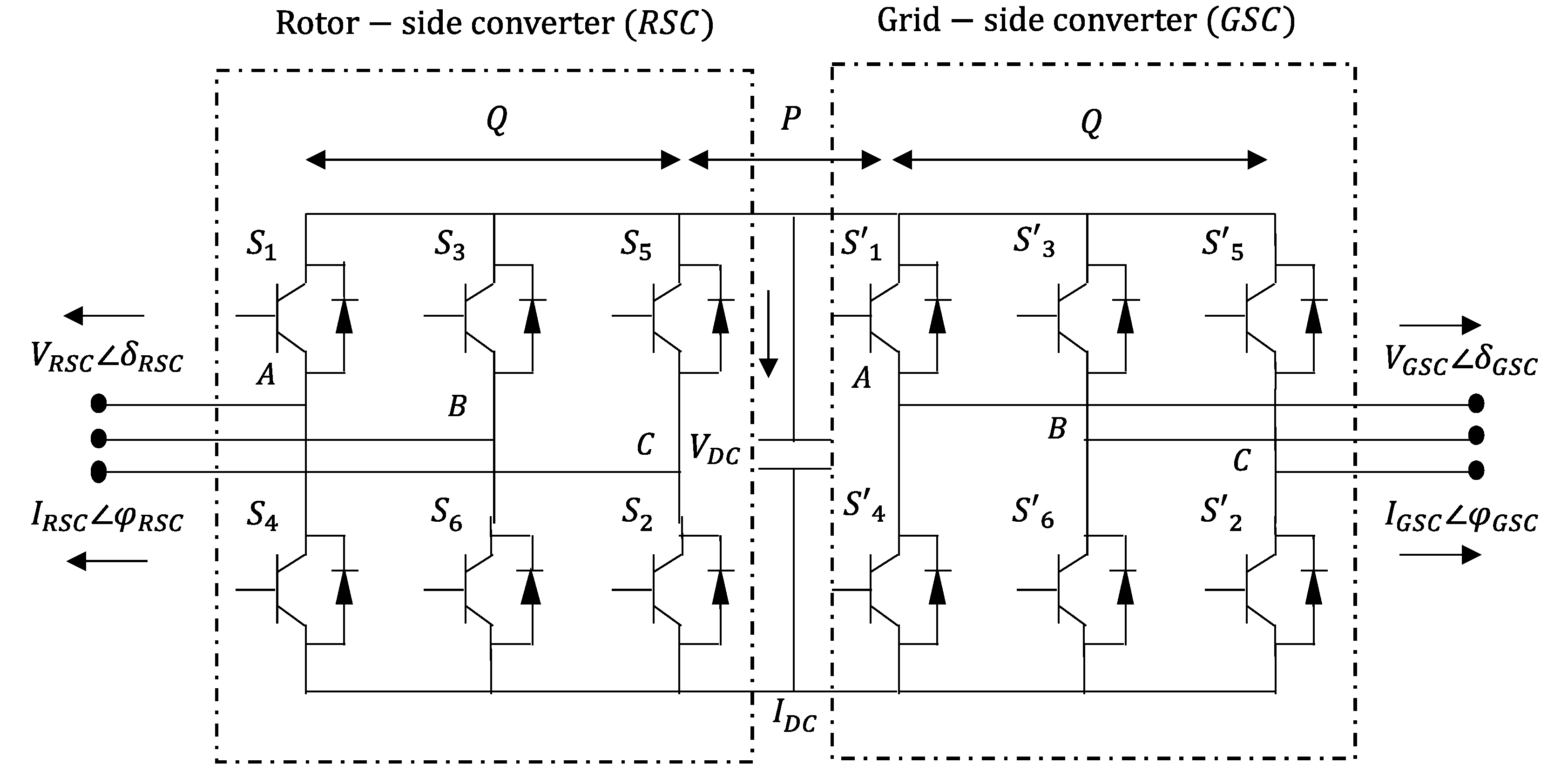
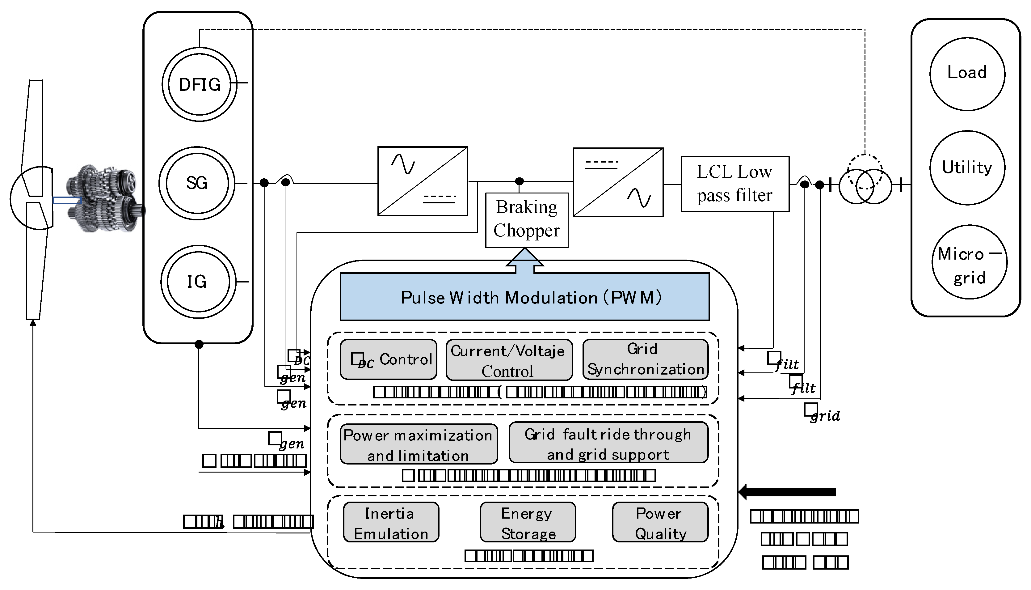
The B2B power converter consists of a rotor–side converter (RSC) and a grid–side converter (GSC) controlled by the PWM, which shares their continuous stage, making a bidirectional converter that is connected in series to a DC bus in parallel with a capacitor, as shown in Figure 1. The GSC controls the active and reactive power flows, keeping the voltage of the DC–link constant within certain limits. Conversely, the RSC controls the speed of rotation and its magnetic flux.

The nomenclature in Figure 1 is as follows: $V_{RSC}$ and ${\delta }_{RSC}$ are the magnitude and angle, respectively, of the electrical machine; $V_{GSC}$ and ${\delta }_{GSC}$ are the magnitude and angle, respectively, of the electrical grid; $V_{CD}$ and $I_{CD}$ are the magnitudes of the voltage and current, respectively, of the DC–link; and $S_1, S_2\dots S_6$ are the switching functions of the RSC and ${S^{\prime }}_1, {S^{\prime }}_2\dots {S^{\prime }}_6$ are the switching functions of the GSC. Finally, P and Q are the active and reactive power, respectively, that flow through the system. This converter type is bidirectional, allowing operation in the four quadrants of the XY plane, and, therefore, both converters operate as rectifiers or inverters. The active and reactive powers through the rotor and stator are controlled by adjusting the amplitude, phase, and frequency of the voltage introduced to the rotor. The RSC provides three-phase voltage at a variable amplitude and frequency, controlling the generator torque and the reactive power exchange between the stator and the electrical grid, while the GSC exchanges the active power with the electrical grid obtained or injected by the RSC from the rotor. The output frequency of the GSC is constant, while the output voltage varies depending on the exchange of the active and reactive powers with the electrical grid. Because of the greater flow of power injected by the stator, the B2B power converter is designed to operate between 25% and 30% of the nominal power of the generator, which allows the design cost and the losses of the generation scheme to be reduced.

On the other hand, for the synchronization and power injection of the B2B power converter into the electrical grid, it is necessary to know the phase’s sequence and to synchronize one phase of the grid through the phase-locked loop (PLL) method. This method requires the grid angle to be estimated to accomplish the necessary transformations using the d–q reference frame of the grid voltage. Determining the correct value of the positive sequence of the fundamental frequency of the grid voltage vector is essential for good control in systems connected to the electrical grid, for which reason there are currently many investigations aimed at achieving PLLs faster and with adequate behavior in the face of grid distortions. Therefore, we consider it important to propose using this type of PLL for the synchronization of the DFIG with the electrical grid, taking into account that the DFIG is very sensitive to voltage dips.

2.1. RSC

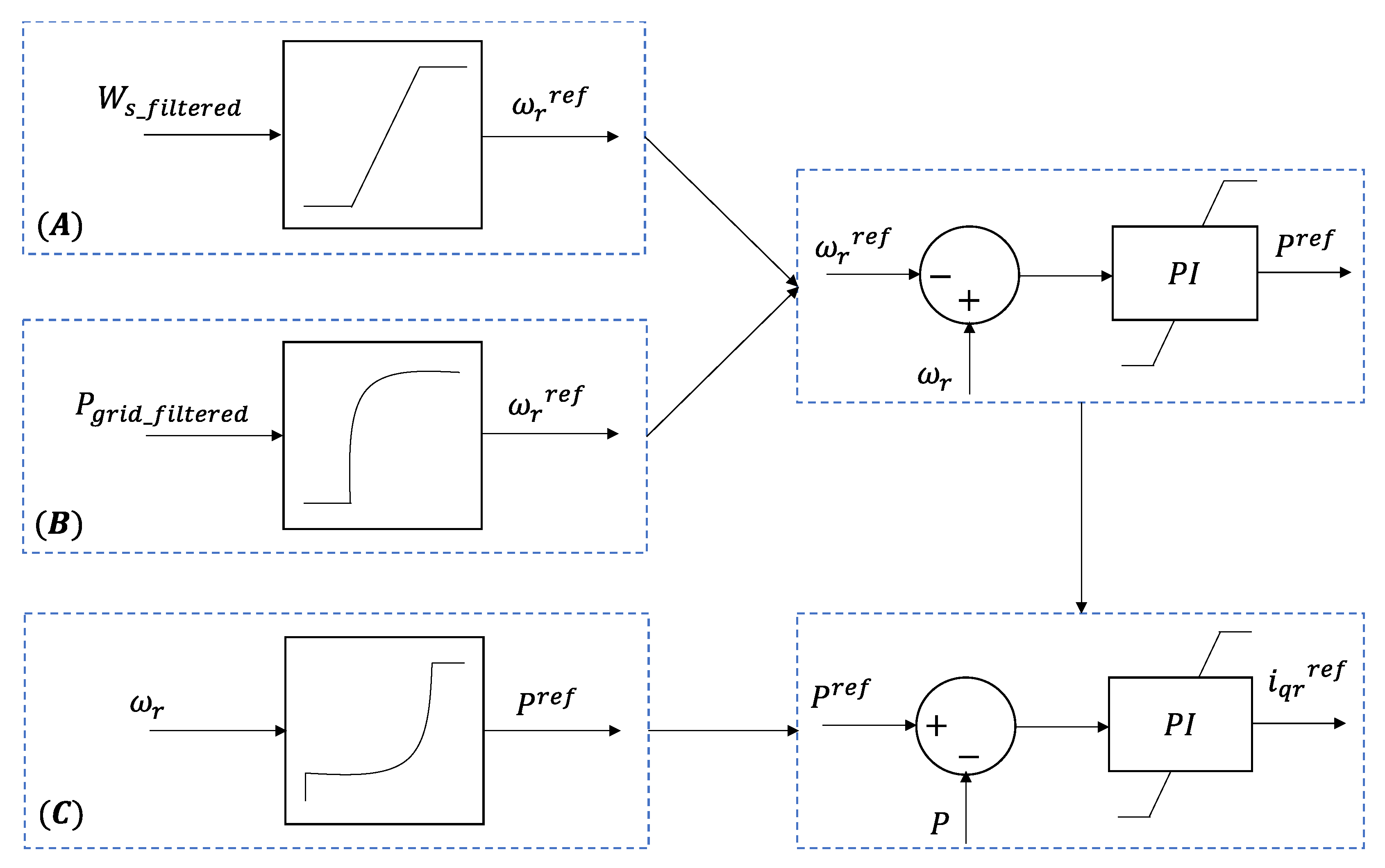
In a DFIG-based wind turbine under a B2B configuration with converters controlled by PWM, the objective of the RSC is to control the amplitude, phase, and frequency of the rotor currents and in turn control the rotor speed, the active power at the stator terminals, and the reactive power at the stator terminals, by using a mobile reference frame, to obtain a decoupling of the currents in two coordinates. The blocks involved in obtaining the reference current for speed and power control may vary, depending on the measurement systems included in the wind turbine and the maximum power extraction method considered.

In Figure 2A, a first block is considered that has the filtered wind speed $\left(W_{s\_filtered}\right)$ as an input signal to later obtain a reference signal for the rotation speed of the generator rotor, ${\omega }_r{}^{ref},$ which is used to obtain the power reference, $P^{ref}$, with which the reference current for the q component of the rotor $i_{qr}{}^{ref}$ is finally generated. The relationship of each component with the active and reactive power depends on the orientation of the reference frame used. On the other hand, in Figure 2B the measured signal is the active power injected into the grid $P_{grid\_filtered}$ from the stator, to obtain ${\omega }_r{}^{ref}$ through this and continue with the same blocks mentioned for the diagram of Figure 2A. Finally, Figure 2C shows the rotation speed of the generator rotor, generating, in turn, stator reference active power through a lookup table. There are also schemes that directly regulate the rotor speed and therefore omit the power regulation stage to obtain the reference current.

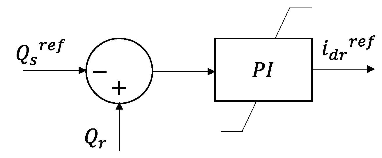
The reference current obtained from the process just described is used to determine the modulation indices of the power converter connected to the rotor and, in this way, generate the current necessary for the desired operation of the machine. The current can be obtained through a PI controller, as shown in Figure 2, or it can be calculated with an analytical expression that depends on the simplifications made in the model. The reactive power injected or absorbed at the stator terminals is controlled with component d of the three-phase rotor current. The implementation of a PI controller like the one shown in Figure 3 is sufficient to fulfill this objective.

2.2. GSC

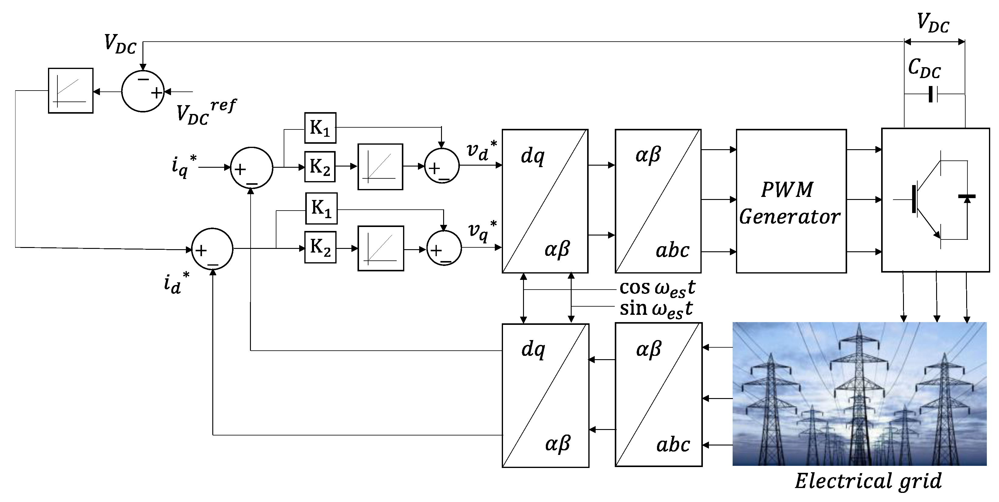
Since the nominal current of the rotor is insufficient for injecting all the reactive power that the machine requires for its operation through the rotor, it is necessary to use GSC, which is responsible for maintaining the voltage of the direct current link regardless of the direction and magnitude of the active power of the rotor. GSC works based on the generation of AC voltages to obtain a current phasor aligned with the grid voltage phasor. For this analysis, the reactive components of the current are considered 0; however, it is possible to use the converter to inject or demand reactive power from the electrical grid. In the active rectifier operating mode, the converter behaves like a boost-type converter since it provides voltage in the DC-link greater than the value of the amplitude of the phase voltages, controlling the real component of the current input to the converter. Additionally, to operate as an inverter, it must inject power into the electrical grid, but in this case and because the value of the three-phase voltage is set by the grid, the converter injects current into the grid to maintain the voltage in the DC-link, which rises when the RSC supplies power to the DC-link.

Considering that the GSC behaves like a voltage source that is connected to the electrical grid, a filter with a known impedance is required so that when generating the output voltage signals through PWM modulation, the current flows from the GSC to the electrical grid or vice versa. The active power transfer by the converter is associated with the real component of the current, so a current phasor with a phase angle of 0° must be obtained for the active rectifier mode of operation and a phase angle of 180° to operate as an inverter that feeds power into the electrical grid. Vector control is used in a reference frame oriented along the position of the stator voltage vector to obtain independent control of the active and reactive power flows between the grid and the converter. The PWM scheme is carried out considering a decoupled regulation strategy, where the current in the d axis regulates the voltage in the DC-link, and the current component in the q axis controls the reactive power. Figure 4 shows the control scheme of the GSC in normal operation. In a similar way to RSC, for the regulation of the voltage in the DC-link and of the reactive power, typical PI controllers with anti-windup are used.

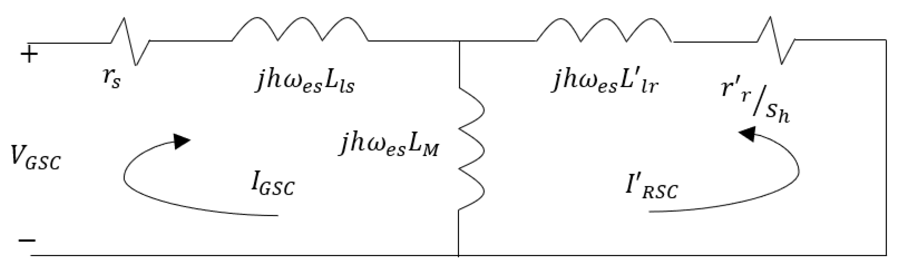
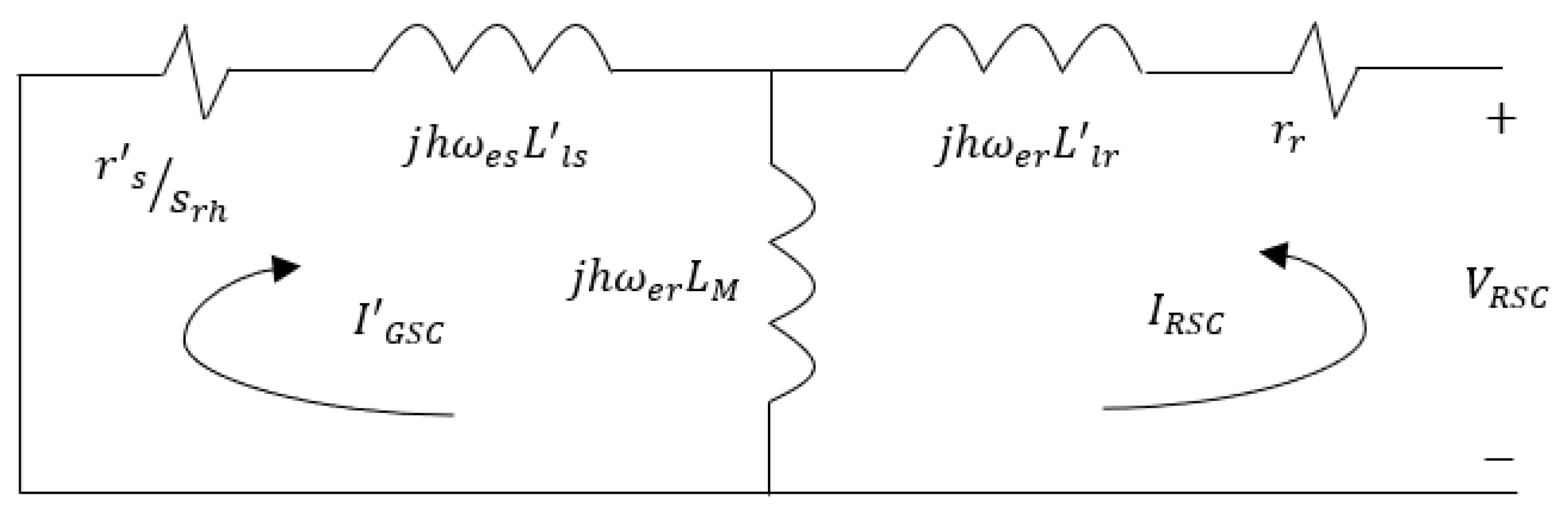
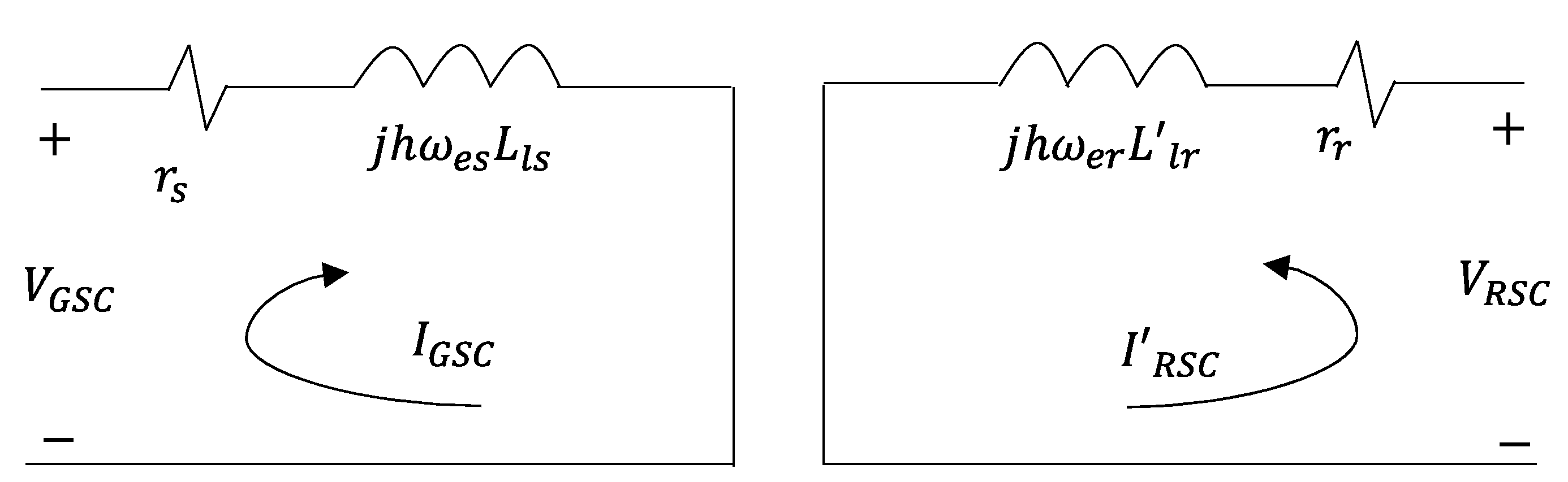
2.3. LCL Filter

The chosen three-phase LCL filter for this research has wye-connected capacitors, and the center wye is not grounded. The GSC output voltages do not refer to ground either but to the central wye of the capacitors. It is important to consider that the main requirements of the LCL filter (low-pass filter) are that it must decouple the power between the grid voltage and the GSC from the voltage source, as shown in Figure 5. It must also filter the differential-mode inverter switching noise from the grid. In addition, it must have low losses and a compact size. Figure 5 shows the location of the filter in the configuration of a wind farm connected to the electrical grid. The nomenclature of the Figure is as follows: $I_{gen}$, $V_{gen}$, and $W_{gen}$ are the current, voltage, and power, respectively, of the generator. Furthermore, $X_{filt}$ and $I_{filt}$ are the reactance and current, respectively, of the filter.

For correct operation, important design aspects must be considered. For example, the value of the capacitor must be limited by the reduction of the power factor to the nominal power (less than 5%), and the total value of the inductance must be less than 10% to limit the DC-link voltage. Similarly, the voltage drop across the LCL filter during operation should limit the intermediate circuit voltage. Regarding the resonance frequency, it must be included in a range between 10 times the line frequency and half the switching frequency in order not to create resonance problems in the lower and upper parts of the harmonic spectrum. Finally, the passive resistance must be chosen as a compromise between the necessary damping and the losses in the system.

3. PWM Switching Techniques

The operation in switched mode of the power converters has made it possible to obtain systems with high efficiency and high-powered density, such as the PWM, which is the basic energy processing technique used in these converters. The continuous increase in the switching speed of power transistors, and the increase in the computing capacity of the DSPs, makes research into increasingly efficient and fast modulation algorithms an area of continuous evolution. 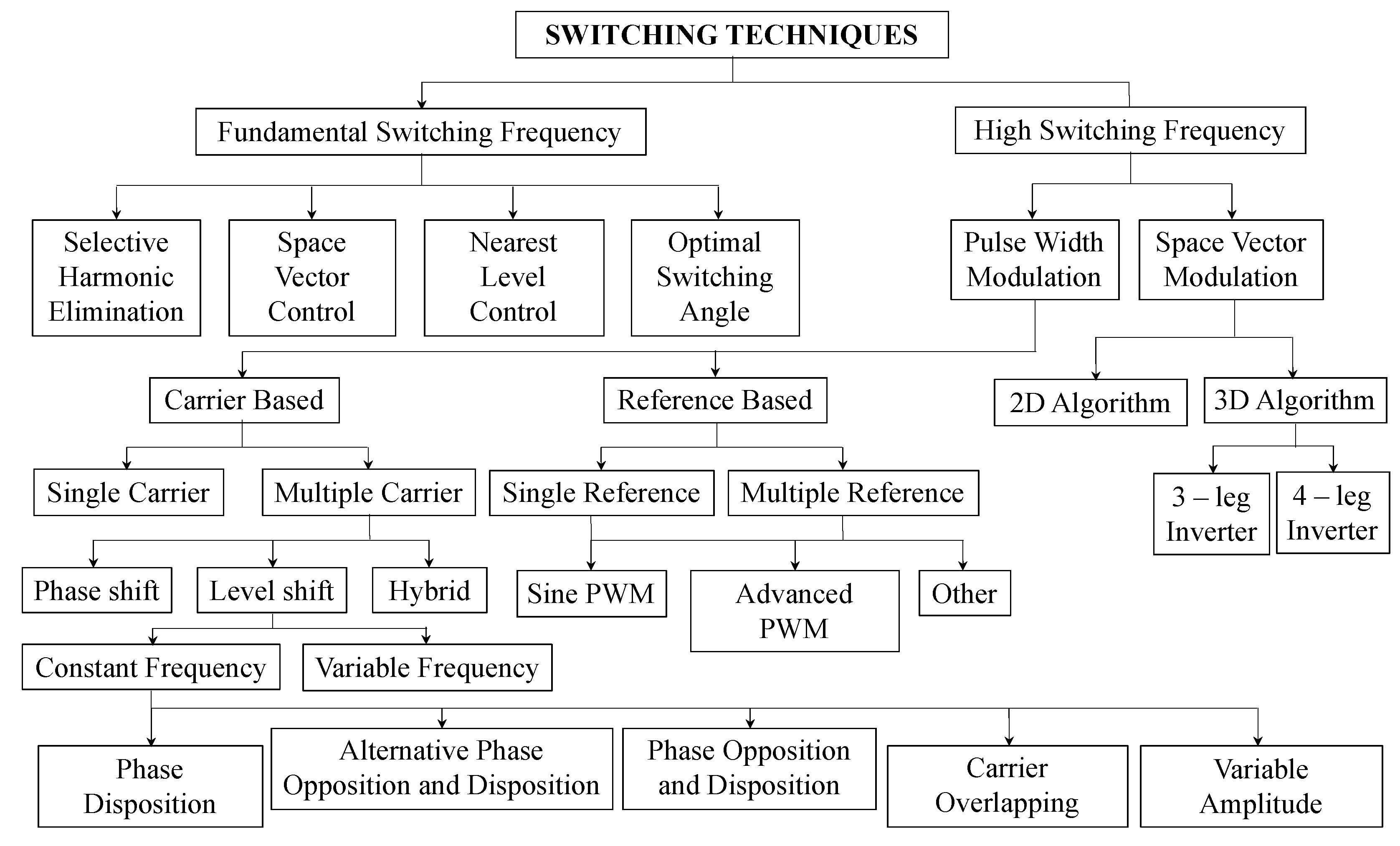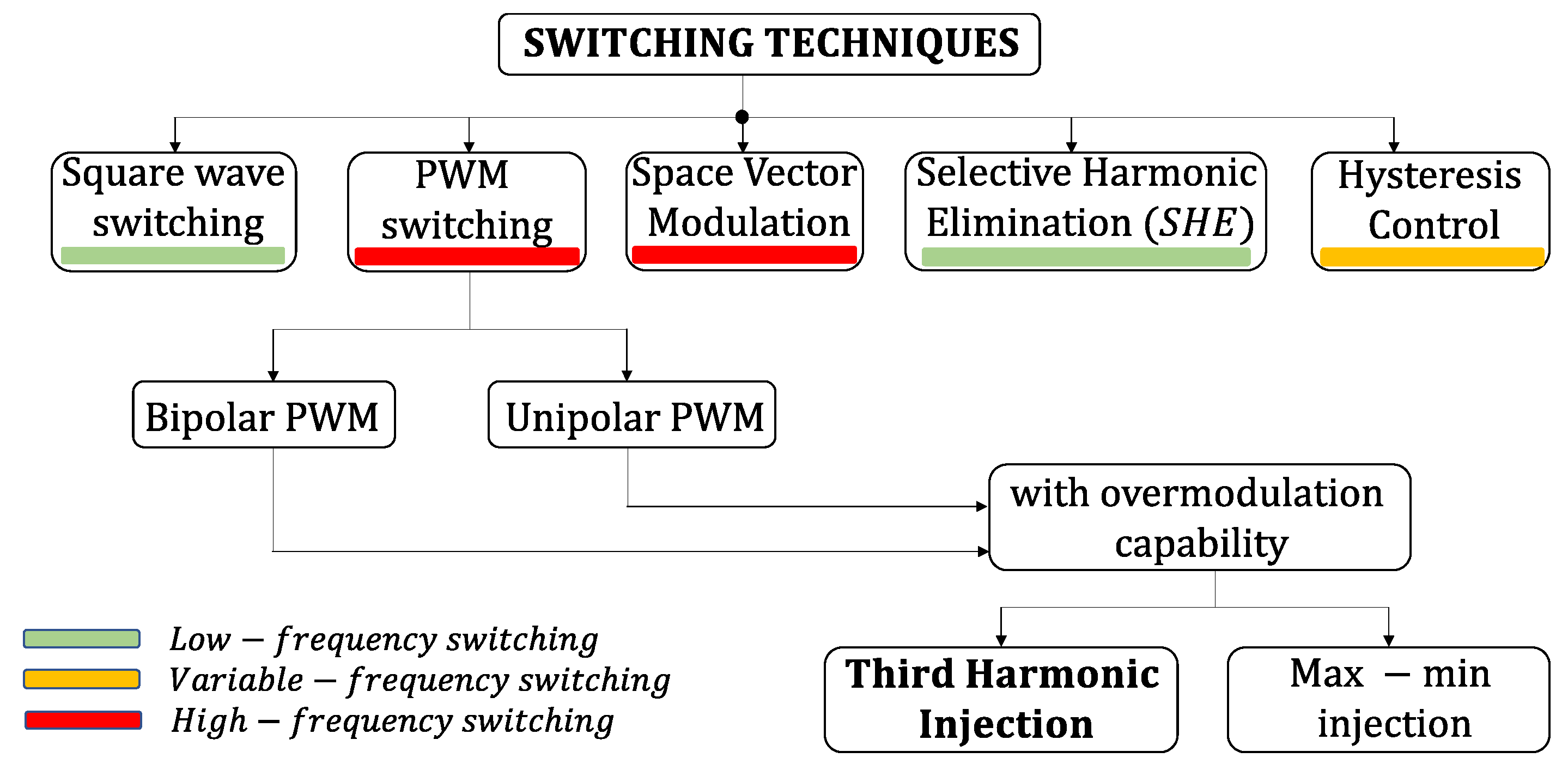Figure 6 shows a schematic diagram of the different PWM switching techniques for power converter applications. In the DFIG, the application of PWM switching techniques for the RSC and GSC can affect the overall performance of the system. The operating principle of B2B power converters is based on the implementation of these PWM switching techniques.

In general, the adoption of these is intended to improve system behavior, improve the THD or dynamic response, reduce switching losses, and increase conversion efficiency, among other improvements. The literature compiles different PWM switching techniques that have been updated over time to achieve greater reliability and efficiency and with less noise in the equipment. Therefore, the specific modulation used is very important for achieving optimum drive performance. PWM switching techniques are a crucial part of the RSC because they are related to the overall efficiency of the entire system. Different types of switching techniques have been proposed in the literature, as summarized in Figure 6. For application in WECSs, the inverter switching concepts are an important part of the control structure. These should provide such characteristics as a wide linear operating range, an increased DC voltage utilization (higher output voltage), low voltage and current harmonic content, low-frequency harmonic signals, the overmodulation operation, and decreased losses through switching. In this section, three switching techniques are analyzed that are applied to the insulated gate bipolar transistors (IGBTs) of the B2B power converter, which are the sinusoidal PWM (SPWM), the third harmonic injection PWM (THIPWM), and the space vector modulation (SVPWM). IGBT switches are used to obtain a higher current-carrying capacity and a high switching frequency. These proposed switching techniques were modeled and simulated in MATLAB-Simulink^® for use with the WECS.

3.1. Sinusoidal PWM (SPWM)

The SPWM switching technique is used to generate activation pulses for the RSC. In this technique, the low-frequency sinusoidal reference waveform is compared with the high-frequency triangle waveforms called carrier waves. When sine and carrier waves intersect, the switching phase changes at that time. In a three-phase system, three low-frequency sinusoidal reference waveforms $\left(V_A, V_B, V_C\right)$ that are 120° out of phase with each other are compared with the triangle wave voltage, resulting in three pulses of switching for three different phases. RSC contains six IGBTs ($S_1$ to $S_6$); two switches will simultaneously operate during one phase and will be connected in series to form one leg of the RSC. Similarly, other switches will operate during the other two phases. The output of each phase is connected to the center of each leg of the RSC, as shown in Figure 1. The output of the comparator provides the control signal or pulses for the power devices connected to the three legs of the RSC. Two single leg switches will work in a complementary manner: when one is on, the other will be off or vice versa. The SPWM switching technique has been used in many applications because of the simplicity of its implementation and the good harmonic distribution of the output voltage spectrum, which concentrates the harmonics because of switching in the carrier frequency and its multiples (dispersing slightly in side bands). This switching technique, however, offers a reduced linear range, which implies a limitation of the DC-link voltage resources.

The high-frequency triangular waveform required for the SPWM switching technique is generated internally in the DSP with an amplitude of 5 V and a frequency of 10 kHz. The DSP compares the sinusoidal waveform and the triangle waveform for generating pulses of widths that are proportional to the amplitude of the sinusoidal wave. Since rotor power is slip dependent, the active power transfer can be controlled by sensing speed and by creating a corresponding phase shift with the help of the DSP. Some drawbacks of the SPWM switching technique are that the THD is higher, the modulation index is lower, and the current produced is lower. It should be mentioned that this technique helps to reduce heat loss in the stator winding.

Regarding harmonic distortion, which is the main topic of this research, the PWM modulation technique pushes the harmonics in the output voltage wave into the high frequency range, around the switching frequency. The multiples of this must be odd integers so that the output voltage contains only odd harmonics. As it is easier to eliminate high frequency harmonics using a passive filter, it is desirable to use a high as possible switching frequency, but there is a disadvantage that the losses in the switching increase proportionally. For the SPWM switching technique with an amplitude modulation index less than 1, however, the fundamental voltage amplitude varies linearly with this modulation index, but the fundamental frequency is lower. When the amplitude modulation index is greater than 1, the amplitude also increases, resulting in overshoot, and the output waveform contains many harmonics. The dominant harmonics in the linear range may not be dominant in the overmodulation; the amplitude of the fundamental component does not vary linearly with the amplitude modulation index.

3.2. Third Harmonic Injection PWM (THIPWM)

The SPWM switching technique is easy to understand and implement, but it is unable to fully utilize the supply voltage of the DC-link. Because of this, the THIPWM appears [16,17,18] as shown in Figure 7. The main objective is to maximize the use of the DC-link and in this way increase the inverter output voltage up to 15.5% with respect to the SPWM switching technique. The THIPWM switching technique is basically used to increase the power factor and control the output voltage of the RSC of the B2B power converter. In addition, this method improves the performance of the RSC, and this is achieved by adding a third harmonic signal in the low-frequency sinusoidal reference signal, thus obtaining an amplitude increase in the waveform of the output voltage.

In the THIPWM switching technique, the addition of the third harmonic means that in one cycle of the sinusoidal wave, three cycles of the harmonic signal must be completed. When the peak of the sinusoidal signal is +1/6 of the third harmonic signal, the amplitude of the fundamental frequency will then be equal to 1. When the peak of the sinusoidal signal is +1/6 of the third harmonic signal, the amplitude of the fundamental frequency will then be equal to 1.155. Adding the third harmonic to the sinusoidal reference leads to a 15.5% increase in the utilization rate of the DC voltage. Since during a third of the period of each leg the RSC is disconnected, the heating of the IGBTs is reduced. The comparator output is used to control the RSC switches exactly the same as in the SPWM switching technique. Similar to the SPWM switching technique, the overmodulation and modulation methods can also be applied to the THIPWM switching technique. It is interesting to observe that the result of adding the third harmonic and the signal at fundamental frequency is smaller in amplitude than the fundamental harmonic. On the other hand, the reference signal occupies two maxima at t = π⁄3 and t = 2π, which are equal to 1.

3.3. Space Vector Modulation (SVM)

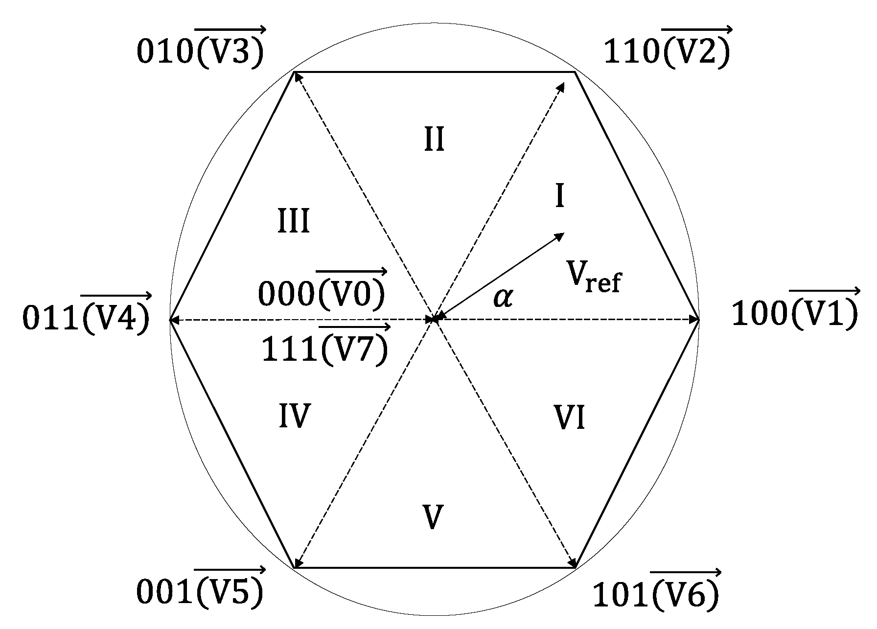
This switching technique performs evaluations of the three-phase reference system to find its resulting vector, which is located and averaged with its adjacent vectors, and to subsequently apply the resulting times of averaging to the appropriate switching sequences for delivering a three-phase sinusoidal voltage. After applying this switching sequence, the three-phase system is re-evaluated, and the sequence begins again. This switching technique applied in the RSC will allow lower harmonic distortion in the output voltages and currents to be obtained, as well as improving the use of the DC-link, obtaining better results than the SPWM switching technique. To implement this technique, it is necessary to know the voltage equations in the abc reference frame and to perform the transformation corresponding to the dq stationary reference frame. As a result of these transformations, we have six active vectors and two null vectors. Active vectors form the characteristic path of the SVPWM, and these vectors supply voltage to the load. The active vectors are separated from each other by 60°. The magnitude of the active vectors is (2⁄3)$V_{DC}$. The null vectors are at the zero point of the complex plane, and they apply 0 V to the charge. For calculating the application time of the different vectors, it is necessary to know the system parameters, such as the switching period, DC-link level, and the offset α. The eight switching combinations correspond to eight stationary voltage vectors in space. The state diagram of six active voltage vectors ${\overrightarrow{V}}_1 \left(100\right)$, ${\overrightarrow{V}}_{2 }\left(110\right)$, ${\overrightarrow{V}}_{3 }\left(010\right)$, ${\overrightarrow{V}}_{4 }\left(011\right)$, ${\overrightarrow{V}}_5 \left(001\right)$, and ${\overrightarrow{V}}_6 \left(101\right)$ and two zero voltage vectors ${\overrightarrow{V}}_0 \left(000\right)$ and ${\overrightarrow{V}}_7 \left(111\right)$ forms a hexagon. The voltage vector diagram of a two-level inverter is shown in Figure 8. The entire space in the two-level inverter is divided into six equal sectors, and the size of each sector is 60°. Each sector is bounded by two active vectors. The zero vectors are located at the origin of the hexagon.

The switching table for the corresponding states is mentioned in

Table 1. Switching table for the three-phase two-level B2B power converter.

State	R		Y		B
	$S_1$	$S_4$	$S_3$	$S_6$	$S_5$	$S_2$
P	1	0	1	0	1	0
N	0	1	0	1	0	1

. The switching state vectors in the two-level inverter are defined by the conducting and non-conducting switches in the power circuit of the inverter.

4. Steady-State Model of the DFIG at Harmonic Frequencies

The scheme discussed in this document is shown in Figure 2. The stator is directly connected to the electrical grid through a three-winding transformer. The rotor is excited by the B2B power converter. The rotor voltage $V_{RSC}$, the rotor frequency $f_r$, and the rotor power $P_r$ depend on the slip s, in which the machine is operating. This last parameter is important, as it defines the operation of the machine. As for the B2B power converter, it makes the variable voltage and the variable frequency of the rotor circuit coincide with those of the electrical grid. Moreover, it facilitates power transfer by introducing a phase change.

Harmonic signals from both the stator and rotor can be generated in the DFIG. These harmonic signals each have their own frequency depending on the voltage source in question: the harmonic frequencies in the stator $f_{sh}=h{f}_{es}$, and harmonic frequencies in the rotor $f_{rh}=h{f}_{er}$, where h is an integer. The frequencies induced in the rotor winding of the machine, because of the harmonics in the stator, cannot be called harmonics of the fundamental frequency of the rotor and vice versa. Therefore, it is advisable to analyze and model the effects on the system from both points of view: from the stator and rotor [19,20,21], respectively.

4.1. Effects of the DFIG Excited by the Stator

To obtain a complete view of the behavior of the machine with respect to the harmonic currents of the stator, first an appropriate equivalent circuit was developed in steady-state seen from the stator (as in Figure 9), which was established in the time-domain. Note that the DFIG was excited from the stator with a harmonic voltage at frequency $f_{sh}$, and the rotor was short-circuited. It should be taken into account that all the DFIG parameters are referred to the stator.

The voltage equation that represents the circuit in Figure 9 is

$$\left[\begin{array}{c}{V}_{GSC}\\ 0\end{array}\right]=\left[\begin{array}{cc}{r}_s+jh{\omega }_{es}\left(L_{ls}+L_M\right)& jh{\omega }_{es}{L}_M\\ jh{\omega }_{es}{L}_M& {r^{\prime }}_r/s_h+jh{\omega }_{es}\left({L^{\prime }}_{lr}+L_M\right)\end{array}\right]\left[\begin{array}{c}{I}_{GSC}\\ {I^{\prime }}_{RSC}\end{array}\right],$$

(1)

where

$$s_h=\frac{\pm h{\omega }_{es}-{\omega }_r}{\pm h{\omega }_{es}}.$$

(2)

For positive sequence harmonics, the sign (+) is used, and for the negative sequence harmonics, the sign (−) is used. In this case, the behavior of the positive sequence harmonics is h = 3k + 1, and the negative sequence is h = 3k − 1 for k = 1, 2, 3, ..., where the most common harmonics are 5, 7, 11, 13, 15, 17, ..., known as characteristic harmonics. From (1), the phasor harmonic currents caused by the harmonic voltage in the stator are obtained: $I_{GSC}=\left|I_{GSC}\right|\angle {\phi }_{GSC}$ and ${I^{\prime }}_{RSC}=\left|{I^{\prime }}_{RSC}\right|\angle {{\phi }^{\prime }}_{RSC}.$ Its representations in the time-domain, in their respective windings, are

$$\begin{array}{c}{i}_{GSC}=\left|I_{GSC}\right|\cos \left(h{\omega }_{es}t+{\phi }_{GSC}\right)\\ i_{RSC}=\left|{I^{\prime }}_{RSC}\right|\cos \left(s_{h}h{\omega }_{es}t+{{\phi }^{\prime }}_{RSC}\mp {\theta }_{eff}\right)\end{array},$$

(3)

where $\mp {\theta }_{eff}$ is $(-)$ for positive sequence and $(+)$ for negative sequences, respectively.

4.2. Effects of the DFIG Excited by the Rotor

For this case, the DFIG was excited from the rotor with a harmonic voltage at frequency $f_{rh}$, and the stator was short-circuited. The DFIG presents the following equivalent circuit with all the parameters related to the rotor, as shown in Figure 10. The voltage equation representing the equivalent circuit in Figure 10 is

$$\left[\begin{array}{c}0\\ V_{RSC}\end{array}\right]=\left[\begin{array}{cc}{r^{\prime }}_s/s_{rh}+jh{\omega }_{er}\left({L^{\prime }}_{ls}+L_M\right)& jh{\omega }_{er}{L}_M\\ jh{\omega }_{er}{L}_M& r_r+jh{\omega }_{er}\left(L_{lr}+L_M\right)\end{array}\right]\left[\begin{array}{c}{I^{\prime }}_{GSC}\\ I_{RSC}\end{array}\right],$$

(4)

where

$$s_{rh}=\frac{\pm h{\omega }_{er}+{\omega }_r}{\pm h{\omega }_{er}}.$$

(5)

The sign (+) and (−) are used for positive and negative sequence harmonics, respectively. From (4), the phasor harmonic currents caused by the harmonic voltage in the rotor are obtained: $I_{RSC}=\left|I_{RSC}\right|\angle {\phi }_{RSC}$ and ${I^{\prime }}_{GSC}=\left|{I^{\prime }}_{GSC}\right|\angle {{\phi }^{\prime }}_{GSC}$. Their representations in the time-domain, in their respective windings, are

$$\begin{array}{c}{i}_{RSC}=\left|I_{RSC}\right|\cos \left(h{\omega }_{er}t+{\phi }_{RSC}\right)\\ i_{GSC}=\left|{I^{\prime }}_{GSC}\right|\cos \left(s_{rh}h{\omega }_{er}t+{{\phi }^{\prime }}_{GSC}\pm {\theta }_{eff}\right)\end{array}$$

(6)

where $\pm {\theta }_{eff}$ is (+) for the positive sequence and (−) for the negative sequence, respectively. Thus, the complete solution for a DFIG is given by the sum of the effects of the two harmonic voltages:

$$\begin{array}{c}{i}_{GSC}=\left|I_{GSC}\right|\cos \left(h{\omega }_{es}t+{\phi }_{GSC}\right)+\left|{I^{\prime }}_{GSC}\right|\cos \left(s_{rh}h{\omega }_{er}t+{{\phi }^{\prime }}_{GSC}\pm {\theta }_{eff}\right)\\ i_{RSC}=\left|I_{RSC}\right|\cos \left(h{\omega }_{er}t+{\phi }_{RSC}\right)+\left|{I^{\prime }}_{RSC}\right|\cos \left(s_{h}h{\omega }_{es}t+{{\phi }^{\prime }}_{RCS}\pm {\theta }_{eff}\right)\end{array}$$

(7)

4.3. Effects of Zero Sequence Harmonics

The harmonic slip equations for both the stator (2) and rotor (5) are used for harmonics that have the same behavior for both positive and negative sequences and are only valid under balanced conditions. For the case of the zero sequence, which corresponds to harmonics h = 3k, the circuit of Figure 10 is not valid because for the zero sequence the DFIG works with the two uncoupled windings, resulting in the circuit of Figure 11, where the voltage equations are represented as

$$\begin{array}{c}{V}_{GSC}=\left(r_s+jh{\omega }_{es}{L}_{ls}\right)I_{GSC}\\ V_{RSC}=\left(r_r+jh{\omega }_{er}{L}_{lr}\right)I_{RSC}\end{array}$$

(8)

From (8), the phasor harmonic currents are obtained because of their respective voltages: $I_{GSC}=\left|I_{GSC}\right|\angle {\phi }_{GSC}$ and $I_{RSC}=\left|I_{RSC}\right|\angle {\phi }_{RSC}$. Its representation in the time-domain, in their respective windings, are

$$\begin{array}{c}{i}_{sh}=\left|I_{sh}\right|\cos \left(h{\omega }_{es}t+{\phi }_{sh}\right)\\ i_{rh}=\left|I_{rh}\right|\cos \left(h{\omega }_{er}t+{\phi }_{rh}\right)\end{array}$$

(9)

Finally, the general solution for balanced conditions including the voltages both at a fundamental frequency and at harmonic frequencies in the stator and in the rotor are given by

$$\begin{array}{c}{i}_{GSC}={\displaystyle \sum _{h=1}^H}\left|I_{GSC}\right|\cos \left(h{\omega }_{es}t+{\phi }_{GSC}\right)+{\displaystyle \sum _{h=1, 3k+1}^H}\left|{I^{\prime }}_{GSC}\right|\cos \left(s_{rh}h{\omega }_{er}t+{{\phi }^{\prime }}_{GSC}+{\theta }_{eff}\right)\\ +{\displaystyle \sum _{h=1, 3k-1}^H}|{I^{\prime }}_{GSC}|\cos \left(s_{rh}h{\omega }_{er}t+{{\phi }^{\prime }}_{GSC}-{\theta }_{eff}\right)\end{array}$$

(10)

$$\begin{array}{c}{i}_{RSC}={\displaystyle \sum _{h=1}^H}|I_{RSC}|\cos \left(h{\omega }_{er}t+{\phi }_{RSC}\right)+{\displaystyle \sum _{h=1, 3k+1}^H}|{I^{\prime }}_{RSC}|\cos \left(s_{h}h{\omega }_{es}t+{{\phi }^{\prime }}_{RSC}-{\theta }_{eff}\right)\\ +{\displaystyle \sum _{h=1, 3k-1}^H}\left|{I^{\prime }}_{RSC}\right|\cos \left(s_{h}h{\omega }_{es}t+{{\phi }^{\prime }}_{RSC}+{\theta }_{eff}\right)\end{array}$$

(11)

From (10) and (11), we obtain the final equations for the complete DFIG model in steady-state. The first sum of (10) is all the harmonics of the current in the stator derived from the non-sinusoidal voltage that includes the harmonics of the positive, negative, and zero sequences. The second summation of (10) is all the harmonics of the current in the rotor of the positive sequence caused by the induction effect. Finally, for the last summation of (10), all the harmonics of the current in the negative sequence rotor are considered, which are also caused by the induction effect. The same representation occurs in (11).

5. Simulation and Experimental Results

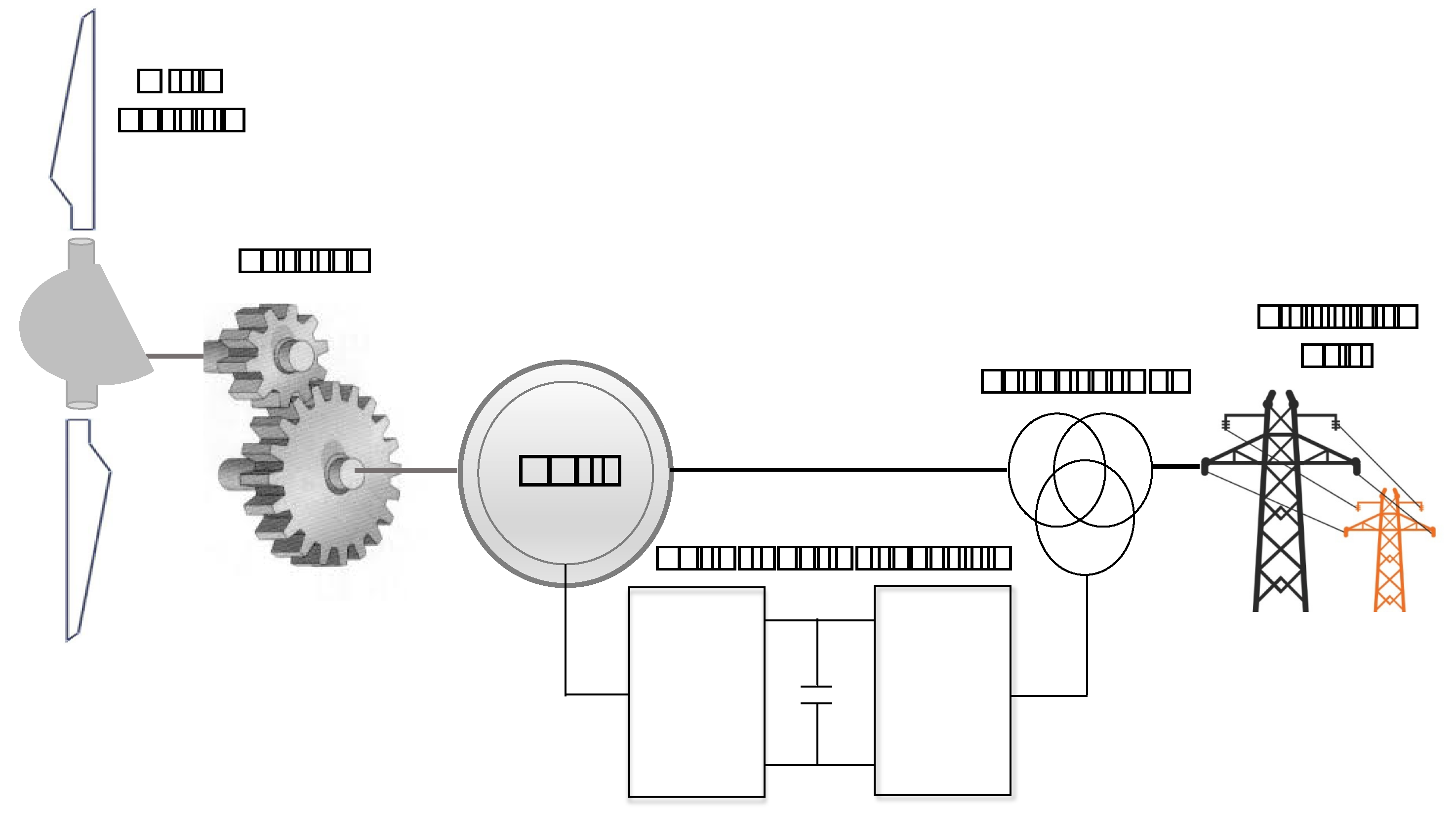
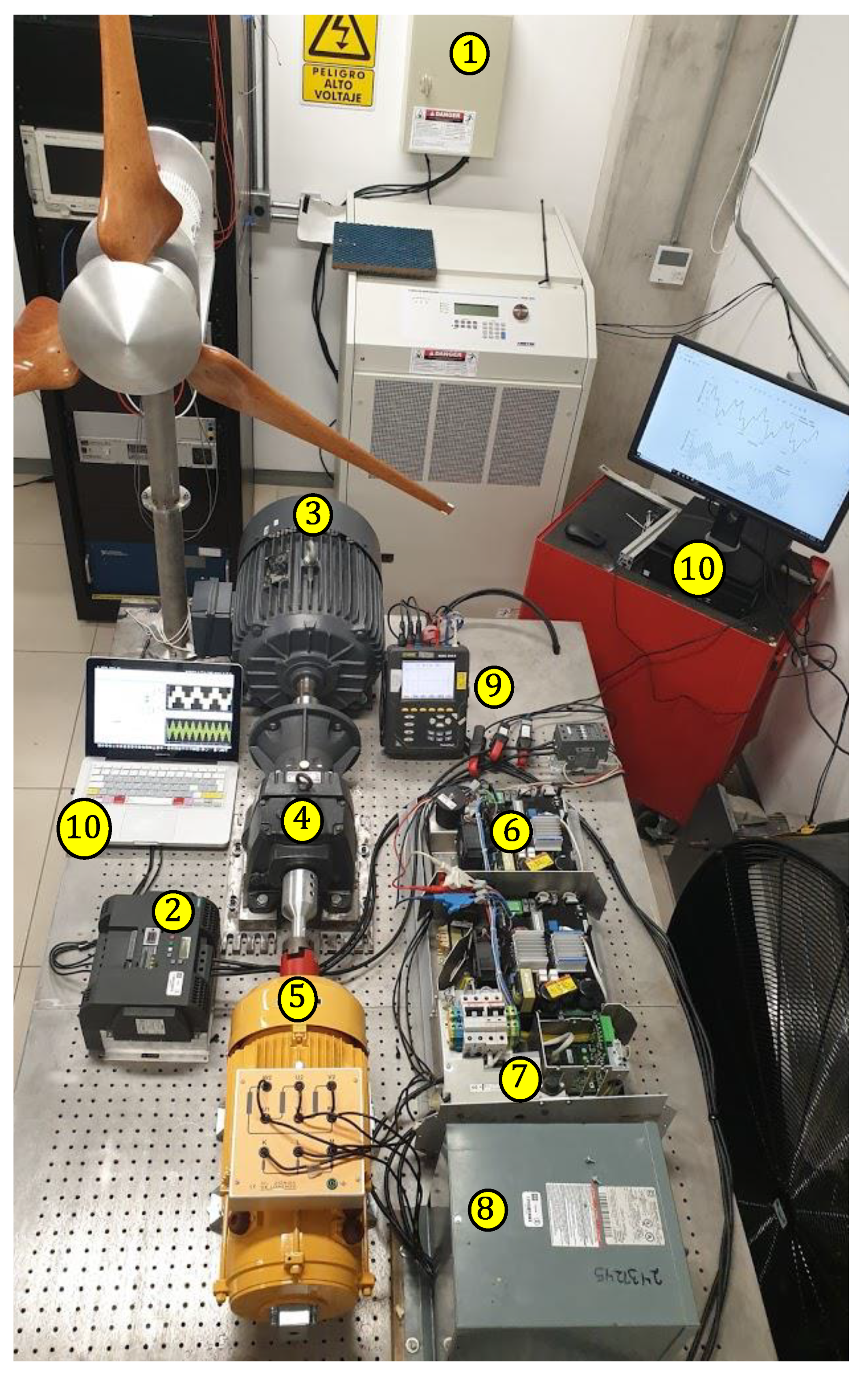
The system under study consisted of a 3-kW DFIG, 230/400 V, and 11.5 A, with parameters that are shown in

Table 2. DFIG parameters.

Parameters	3 kW-DFIG
Poles number	4 poles
Inertia constant	$0.089 \mathrm{kg}/{\mathrm{m}}^2$
Nominal line current	5.8 A
Nominal line-to-line voltage	230/400 V
Nominal torque	11.9 N × m
Nominal frequency	60 Hz
$\mathrm{Stator} \mathrm{resistance}, r_s$	0.435 Ω
$\mathrm{Rotor} \mathrm{resistance}, r_r$	0.816 Ω
$\mathrm{Stator} \mathrm{inductance}, L_{ls}$	2 mH
$\mathrm{Rotor} \mathrm{inductance}, L_{lr}$	2 mH
$\mathrm{Magnetizing} \mathrm{inductance}, L_M$	69 mH
Rotor speed	1500 rpm

. The DFIG was driven by a gearbox (4.5:1 transmission). A 10-HP motor was used as the main motor instead of a wind turbine to simulate different wind speeds. The motor speed was regulated by an adjustable frequency drive (AFD) of 480 V and 35.5 A. The stator, as shown in Figure 12, was connected directly to the electrical grid through a three-phase transformer of 440 V, while the rotor was connected to the B2B power converter. The purpose of the converter was to convert the rotor voltage to DC voltage. The magnitude of that voltage varied with slip. A capacitor in the DC-link was connected to the output of the B2B power converter to regulate the output voltage. This voltage had to be converted to electrical grid values by the GSC. Given the scope of this work, it was not necessary to implement a more detailed model of the power electronic equipment involved.

The schematic diagram of the experimental prototype is shown in Figure 13. The detailed parameters of the experimental prototype equipment are listed in

Table 3. Parameters of the experimental setup.

No.	Equipment	Characteristics
1	Power supply	450 V, 18 A.
2	Adjustable Frequency Drive	480 V, 35.5 A, Motor: 20 HP.
3	Squirrel Cage Motor	10 HP, 460 V, 17.3 A.
4	Gearbox	Ratio 4.5:1, 12.5 kW
5	DFIG	$3-\mathrm{kW}, 230/400 \mathrm{V} \Delta /\mathrm{Y}$, 4.5 A.
6	Rotor side converter (RSC)	IGBT type: 1MBH30D, 4.5 kW, 5 kHz
7	Grid side converter (GSC)	IGBT type: 1MBH30D, 4.5 kW, 2.5 kHz
8	Three-phase transformer	480 V, Y–Y connection.
9	Power Quality Analyzer	PowerPad, Mod. 3945-B.
10	Computer	MATLAB/Simulink® 2020a software

.

In this experimental test, the RSC output voltage was obtained using a DSP TMS 320F28, which has the ability to interact with MATLAB-Simulink^®, thus reducing the efforts in the generation of pulses. This can be programmed according to the requirements of the MATLAB-Simulink^® software. The DSP is programmed to produce pulses in the IGBTs’ gate by comparing a 2.5 kHz triangular carrier wave and a 60 Hz reference sinusoidal wave. The amplitude of the reference wave decides the generated AC voltage amplitude, and the frequency of the reference wave adjusts the frequency of the AC voltage generated. Thus, the pulses generated by the DSP feed the optocoupler, which amplifies the voltage level to a level required for activating the IGBTs by isolating the DSP from the power circuit. This DSP has six ePWM (enhanced PWM) modules that can generate the desired PWM signals. It is worth mentioning that digital control using a DSP provides precision and improves system performance.

Below are three case studies where the different analyzed PWM switching techniques were implemented in the B2B power electronic converter, namely SPWM, THIPWM, and SVM, which were analyzed in the previous sections. MATLAB-Simulink^® was the software used for the analysis and implementation of the different switching techniques presented. The results were then validated with the help of the experimental prototype, where it should be noted that the results obtained with the proposed model in steady state were compared with those obtained in the experimental test, resulting in current waveforms both in the stator and in the rotor, which were similar to the magnitude and phase angle.

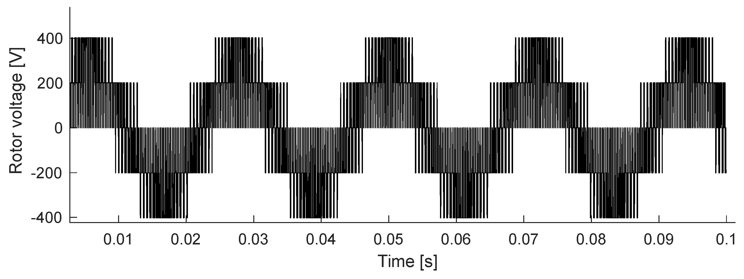
5.1. Case Study 1: 3 kW DFIG-Based Wind Turbine Excited by Nonsinusoidal Voltage in the Rotor Generated by a B2B Power Converter Applying the SPWM Switching Technique

For the first case study, the stator of the DFIG was excited by a sinusoidal three-phase voltage of 400 V at 60 Hz coming from the electrical grid, while the rotor was excited by a nonsinusoidal three-phase voltage of 400 V at 45 Hz generated by the B2B power converter. For this case, the SPWM switching technique was used to activate the RSC switches and generate the rotor voltage waveform shown in Figure 14.

The harmonic components of the rotor voltage are listed in

Table 4. Harmonic components of the rotor voltage for test case 1. THD = 36.7%.

	Harmonic Components
	5th	7th	11th	13th	17th	19th	23th	25th	29th	31th
Volt. (%)	7.79	5.26	3.30	2.61	2.44	2.03	1.88	1.32	1.37	1.40
$\mathrm{Deg}. (°)$	$-$11.2	13.7	208.5	$-$17.2	53.1	41.8	$-$28.8	142.2	23.4	$-$129

. In the SPWM switching technique, the reference wave was compared with a sinusoidal wave to generate pulses at 2.5 kHz. For lower switches, pulses with a phase difference of 180° were provided to avoid short-circuits.

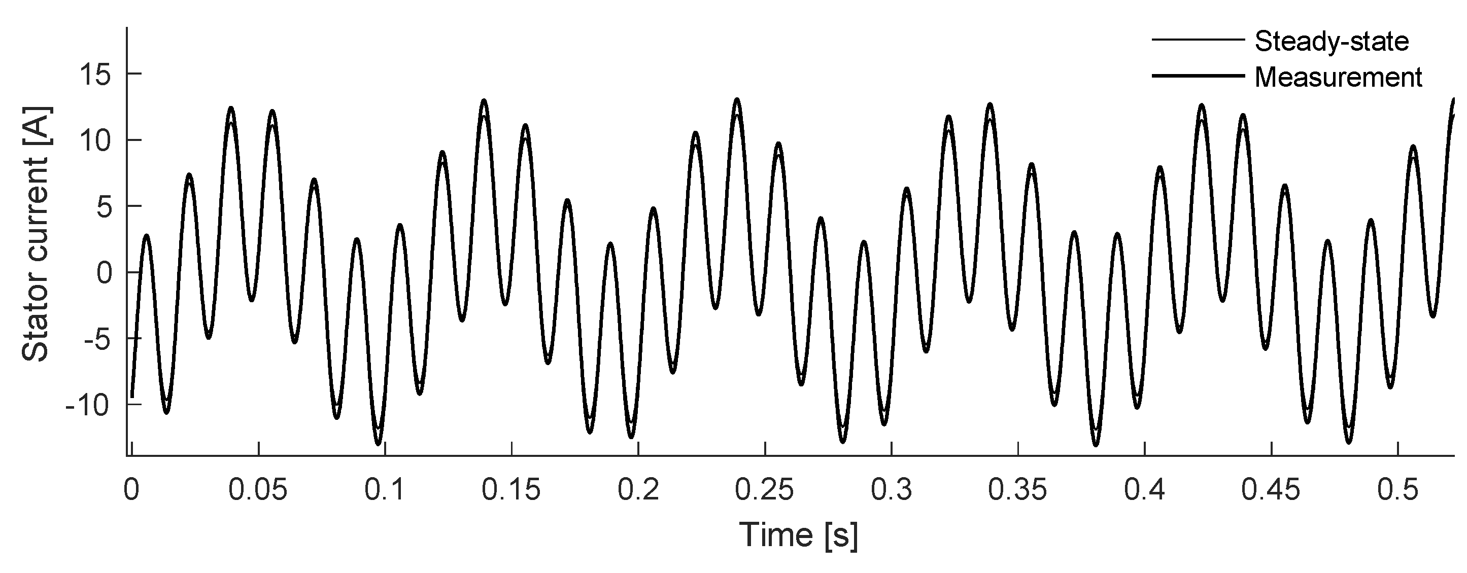
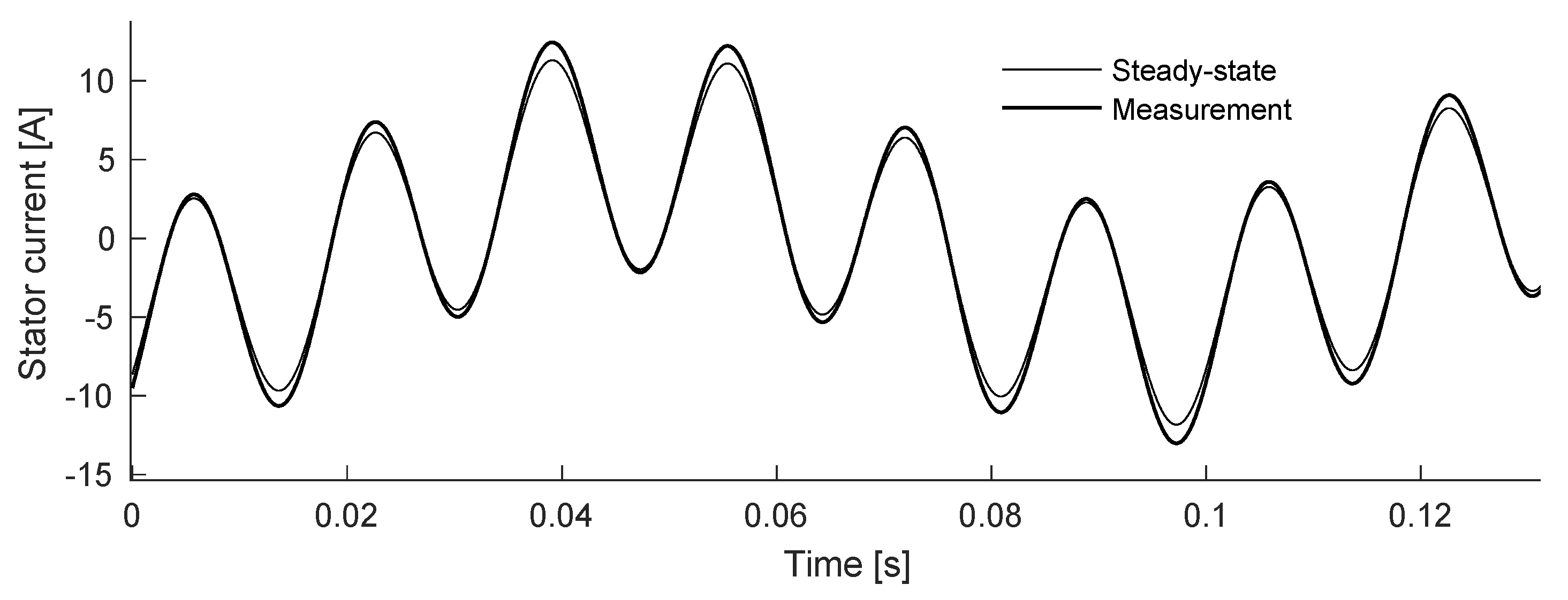
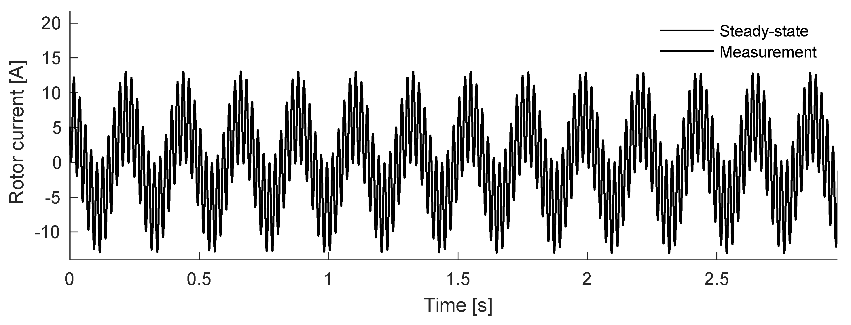
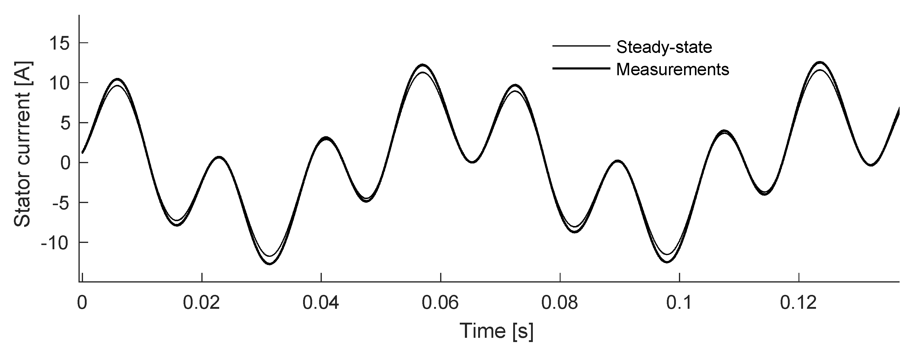
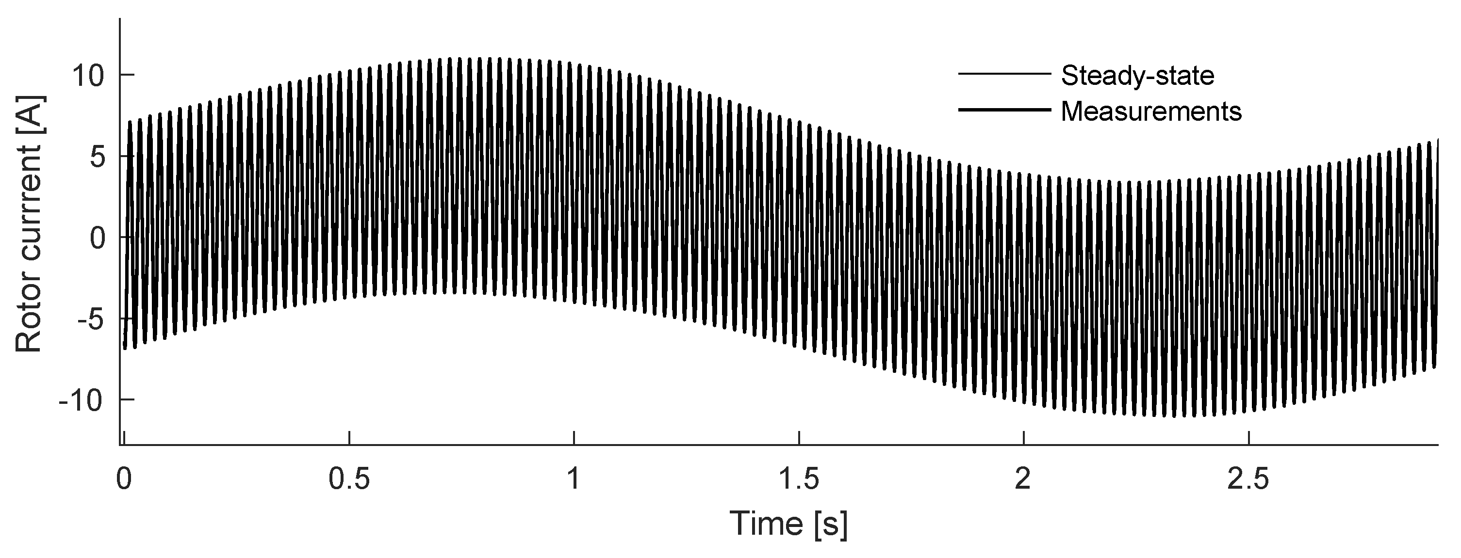
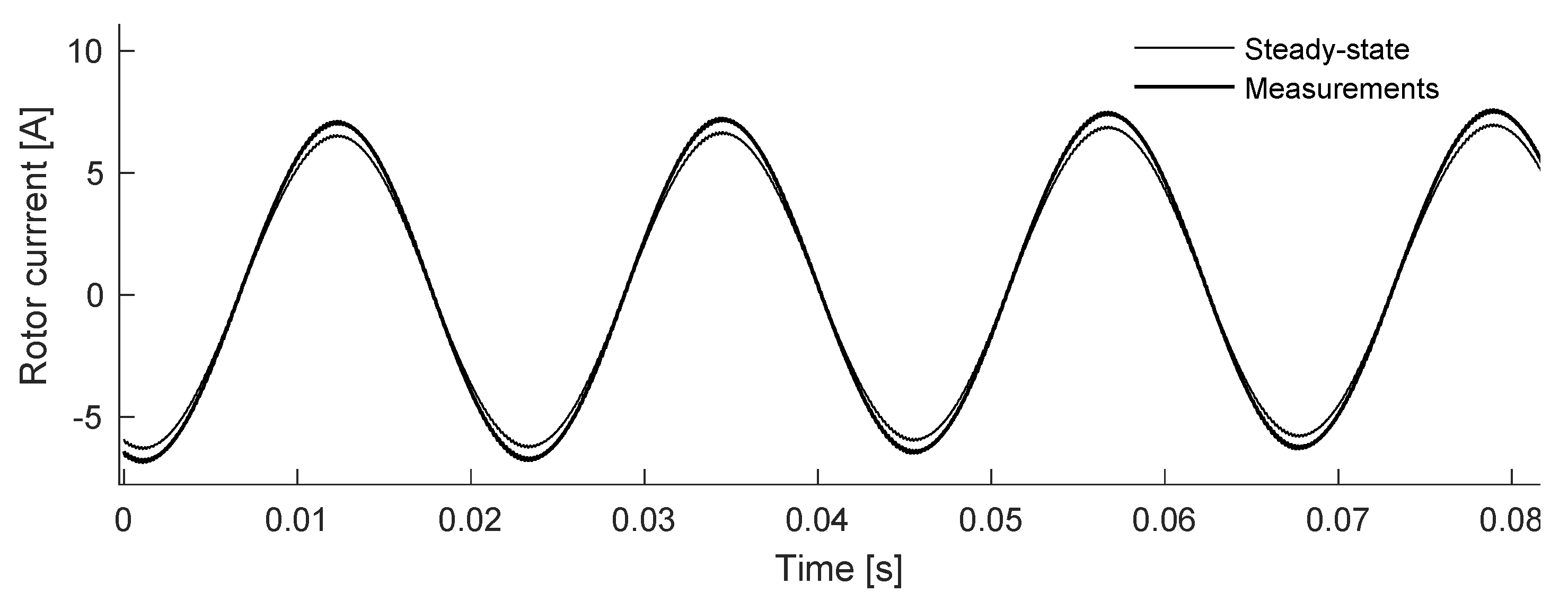
Figure 15, Figure 16, Figure 17 and Figure 18 show the current waveforms in the stator and rotor, respectively. Both figures show the results obtained from the proposed model as well as those obtained experimentally. For all case studies, a wind speed of 14 m/s was considered. The only disturbances to the system present in the simulations were wind variations, so the implementation of an RSC protection system (crowbar) was unnecessary. It should be noted that a nonsinusoidal three-phase voltage will generate harmonic currents in the GSC, as well as in the stator and rotor of the machine.

The harmonic currents generated in a DFIG are mainly caused by harmonic voltages in the electric grid, by spatial harmonics caused by the design of the machine or by the behavior of the RSC switching techniques. For this case, because of the distribution of the rotor winding, the magnetic flux and the flux linkage of the induction machine were distributed in a sinusoidal way, causing the stator current induced by the rotor to contain harmonic components. The amplitude of these harmonic currents largely depends on the type of winding of the machine and the power level since they tend to decrease in high power machines [19].

From the results obtained in this case study we can see that the harmonic currents in the stator induced harmonic currents in the rotor, although with different frequencies. These induced current signals cannot be called harmonic because they are not integer multiples of the fundamental frequency, but they are called interharmonic and contribute to torque oscillations and voltage fluctuations in the DC-link. The impedance in the rotor was dominated by the inductive term, which increased with the harmonic order, with the magnitude of the harmonics of the rotor current being very small. The behavior of the machine was slightly different as far as lower order harmonics are concerned, particularly the fundamental negative sequence component. It should be mentioned that the harmonic distortion of the rotor current varied with respect to the wind speed: that is, for high wind speeds (greater than 14 m/s) where the fundamental rotor voltage was small, the THD became very high.

For this case study, the harmonic currents in the rotor appeared at the following frequencies: $f_{rh}$=(6h ± 1)s$f_{es}$ where h = 0,1,2,3, ... that is, at the 5th, 7th, 11th, 13th, 17th, 19th, ... harmonic of the fundamental frequency. These harmonic currents in the rotor established rotating magnetic fields in the air gap, inducing their corresponding frequencies in the stator. The current distortion in the DC-link introduced by the GSC was also reflected in the rotor currents, which caused additional harmonics. The same principle was applicable to the harmonics of the GSC, which appeared at the frequencies $f_{sh}$=|(6m ± 1)s ± 6hs|$f_{es}$, h, m = 0,1,2,3, ..., with the integer harmonic components presented in

Table 5. Summary of harmonic currents for case study 1.

STATOR CURRENT				ROTOR CURRENT
Seq.	Magn.	Angle	Freq. (Hz)	Seq.	Magn.	Angle	Freq. (Hz)
$+$	100%	$-$$48.2°$	60	$+$	100%	$251.4°$	45
$-$	1.82%	$-1.7°$	300	$-$	0.76%	$179.3°$	225
$+$	1.30%	$-1.2°$	420	$+$	0.54%	188.4°	315
$-$	1.32%	$53.8°$	495	$-$	0.44%	$91.7°$	378
$+$	1.06%	$-0.8°$	516	$+$	0.37%	$-$$17.2°$	486
$-$	0.89%	$61.1°$	492	$-$	0.34%	$81.9°$	495
$+$	0.83%	$55.9°$	660	$+$	0.29%	$180°$	585
$-$	0.7%	$-$$30.2°$	780	$-$	0.23%	$-$$32.7°$	657
$+$	0.63%	$29.1°$	864	$+$	0.21%	$66.5°$	747
$-$	0.54%	$10.1°$	1008	$-$	0.16%	$19.7°$	765
$+$	0.53%	$0.2°$	1020	$+$	0.15%	$28.1°$	855
$-$	0.48%	$-$$10.9°$	1140	$-$	0.14%	$180.3°$	1035
$+$	0.41%	$202.5°$	1320	$+$	0.13%	$-$$40.2°$	1125
$-$	0.4%	$332°$	1380	$-$	0.13%	$73.9°$	1197
$+$	0.36%	$-$$110.2°$	1500	$+$	0.12%	51.8°	1296
$-$	0.32%	$50.2°$	1704	$-$	0.11%	$30.6°$	1305
$+$	0.28%	$28°$	1740	$+$	0.1%	$-181.4°$	1395
${\mathrm{THD}}_{\mathrm{i}}=13.39\%$				${\mathrm{THD}}_{\mathrm{i}}=37.28\%$

For $h\ne 0$, the interharmonics of the current were produced in cascade, and these were quite significant depending on the slip of the machine. Since slip was not an integer, the harmonic content of the stator current consisted mainly of subharmonics and interharmonics, creating unwanted effects on the electrical grid. For example, low frequency subharmonics appeared as unidirectional components superimposed on the phase currents, while subharmonic and interharmonic components close to the grid frequency could have an undesirable effect on the magnitude of the stator current.

An important measure of the performance of this system is the THD reduction in both the stator and rotor current. Table 5 presents the global results of the harmonic currents in the DFIG for each winding case study 1.

5.2. Case Study 2: 3 kW DFIG-Based Wind Turbine Excited by a Nonsinusoidal Voltage in the Rotor Generated by a B2B Power Converter Applying the THIPWM Switching Technique

In this case, the stator of the DFIG was excited with a balanced three-phase sinusoidal voltage of 400 V at 60 Hz, while the rotor was excited by a nonsinusoidal three-phase voltage of 400 V at 45 Hz generated by the B2B power converter. The THIPWM switching technique was used to activate the RSC switches and generate the rotor voltage waveform shown in Figure 19.

The harmonic components of the rotor voltage are listed in

Table 6. Harmonic components of the rotor voltage for case study 2. THD = 13.67%.

	Harmonic Components
	5th	7th	11th	13th	17th	19th	23th	25th	29th	31th
Volt. (%)	6.7	4.8	3.13	2.5	1.64	1.6	1.3	1.58	1.08	1.21
$\mathrm{Deg}. (°)$	169.1	17.5	$-$92.7	82.1	−48.7	95.1	63.6	−72.9	80.1	$-$199

. Figure 20, Figure 21, Figure 22 and Figure 23 show the stator and rotor current waveforms, respectively. Both figures show the results obtained from the proposed model as well as those obtained experimentally.

When applying the THIPWM technique, it can be noticed that there was a reduction in the THD of both the voltage and the current.

Table 7. Summary of harmonic currents for case study 2.

STATOR CURRENT				ROTOR CURRENT
Seq.	Magnitude	Angle	Freq. (Hz)	Seq.	Magnitude	Angle	Freq. (Hz)
$+$	100%	$-$$34.2°$	60	$+$	100%	$-$$30.9°$	45
$-$	0.94%	$186.4°$	300	$-$	0.51%	$-$$1.7°$	225
$+$	0.67%	$47.8°$	420	$+$	0.32%	6°	315
$-$	0.57%	$12.9°$	500	$-$	0.25%	$4.9°$	392
$+$	0.46%	$-$$8.1°$	620	$+$	0.21%	$24°$	461
$-$	0.43%	$33.8°$	660	$-$	0.2%	$-$$113.7°$	495
$+$	0.36%	$92.6°$	780	$+$	0.17%	$35°$	585
$-$	0.32%	$-$$77.3°$	880	$-$	0.15%	$3.3°$	641
$+$	0.28%	$-$$62.1°$	1000	$+$	0.13%	$-$$66.9°$	750
$-$	0.26%	$288°$	1020	$-$	0.12%	$29.8°$	765
$+$	0.25%	182.5°	1140	$+$	0.1%	$12.1°$	840
$-$	0.23%	$-0.1°$	1240	$-$	0.09%	$-$$62.2°$	1005
$+$	0.2%	$85.1°$	1380	$+$	0.09%	$2.5°$	1035
$-$	0.19%	$-$$23.6°$	1500	$-$	0.08%	$-$$0.34°$	1125
$+$	0.18%	$271.8°$	1600	$+$	0.07%	$42.7°$	1260
$-$	0.16%	$100.9°$	1740	$-$	0.07%	$179.3°$	1305
$+$	0.15%	$-$$55.7°$	1860	$+$	0.06%	$-98.2°$	1395
${\mathrm{THD}}_{\mathrm{i}}=8.76\%$				${\mathrm{THD}}_{\mathrm{i}}=21.05\%$

presents the global results of the harmonic currents in the DFIG for each winding. It should be noted that the waveforms of the stator and rotor currents presented in this case study were obtained from the harmonic components shown in the Table, which were obtained from Equations (10) and (11) mentioned in the previous section.

THIPWM was employed to reduce the total harmonic distortion (THD) and make the B2B power converter suitable for grid connection, by synchronizing the inverter voltage with the grid voltage. In addition, this technique increases the efficiency of the B2B power converter. Simulation results shown in Figure 21 and Figure 23 validate the developed model and the proposed system.

By applying this switching technique, currents with low harmonic distortion can be obtained in the stator, in the rotor, and in the electrical grid or load, since the GSC controls the power flow between the rotor and the electrical grid or load, acting as an active filter, and thus can compensate for the harmonics injected by the stator to the grid. On the other hand, the complete system is made to operate at the unity power factor. This is often mentioned as an advantage because the capacitor in the DC-link allows separate control of the two inverter/rectifiers. Note that the distortions in the current because of the carrier frequency increase the ohmic losses in the windings of the machine. Simultaneously, the voltage harmonics increase the losses in the magnetic core, causing an increase in the operating temperature in this type of converter.

5.3. Case Study 3: 3 kW DFIG-Based Wind Turbine Excited by a Nonsinusoidal Voltage in the Rotor Generated by a B2B Power Converter Applying the SVPWM Switching Technique

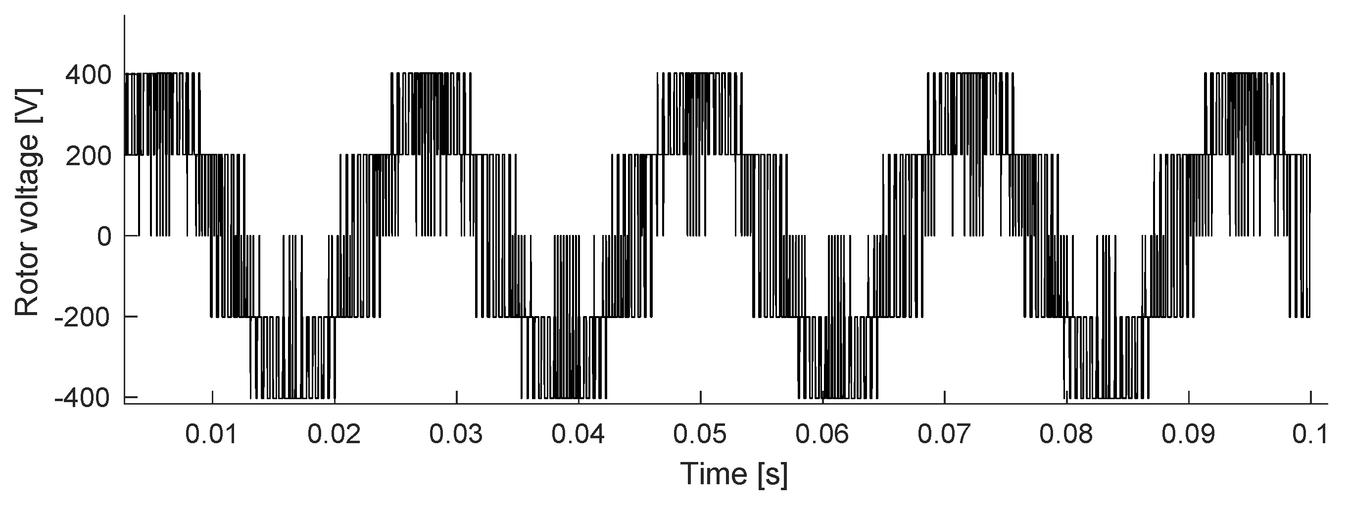
In this case, the stator of the DFIG was excited with a balanced sinusoidal three-phase voltage of 400 V at 60 Hz, while the rotor was excited with a nonsinusoidal three-phase voltage of 400 V at 45 Hz generated by the B2B power converter. The switching technique applied to activate the RSC switches and generate the rotor voltage waveform shown in Figure 24 was SVPWM. The harmonic components of the rotor voltage are listed in

Table 8. Harmonic components of the rotor voltage for case study 3. THD = 8.7%.

	Harmonic Components
	5th	7th	11th	13th	17th	19th	23th	25th	29th	31th
Volt. (%)	7.92	13.52	4.72	3.34	1.69	1.88	1.68	2.49	0.88	1.51
$\mathrm{Deg}. (°)$	18.3	$-$75	225.3	90.2	155.4	$-$92.6	169.8	213.9	$-$17.9	147

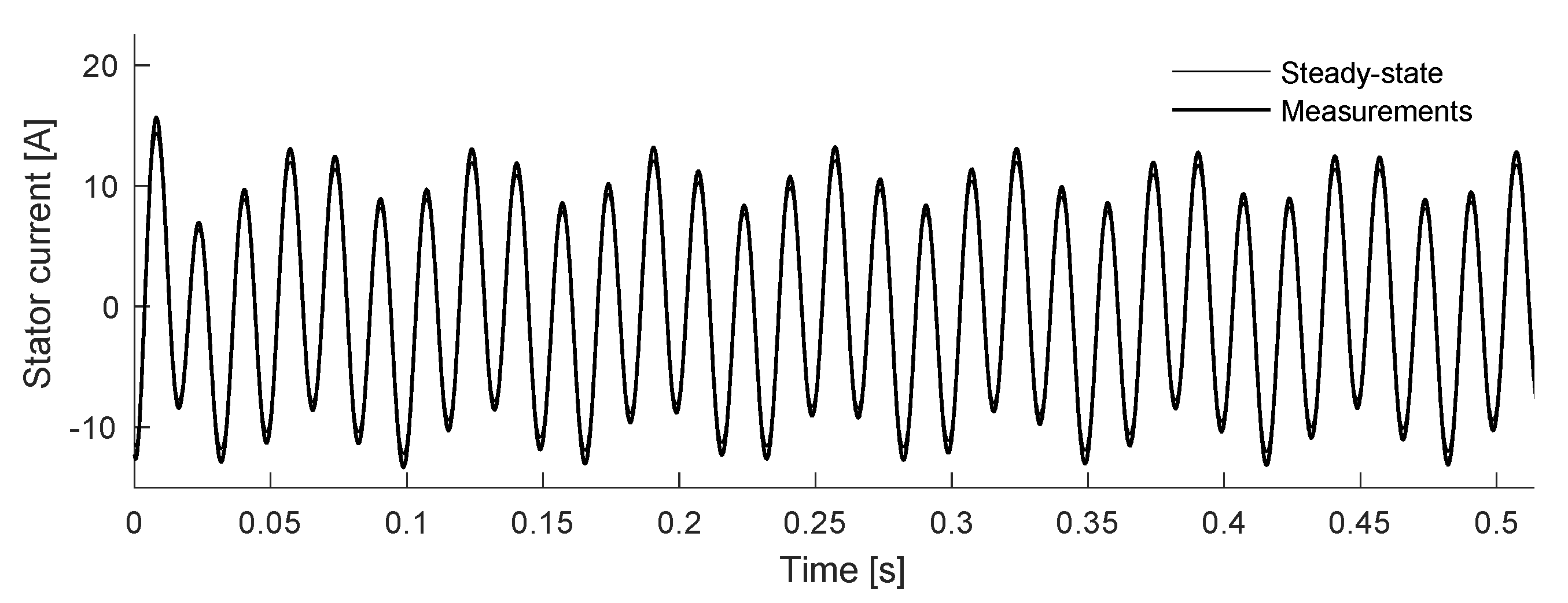
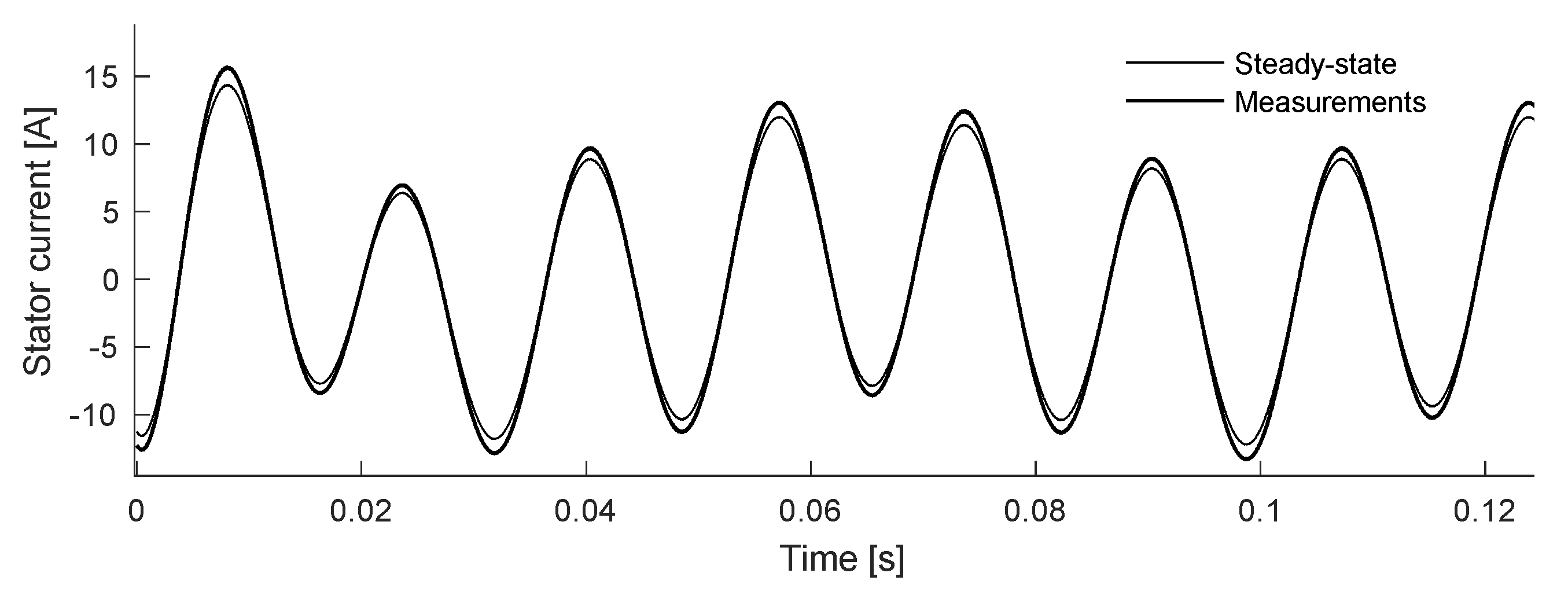
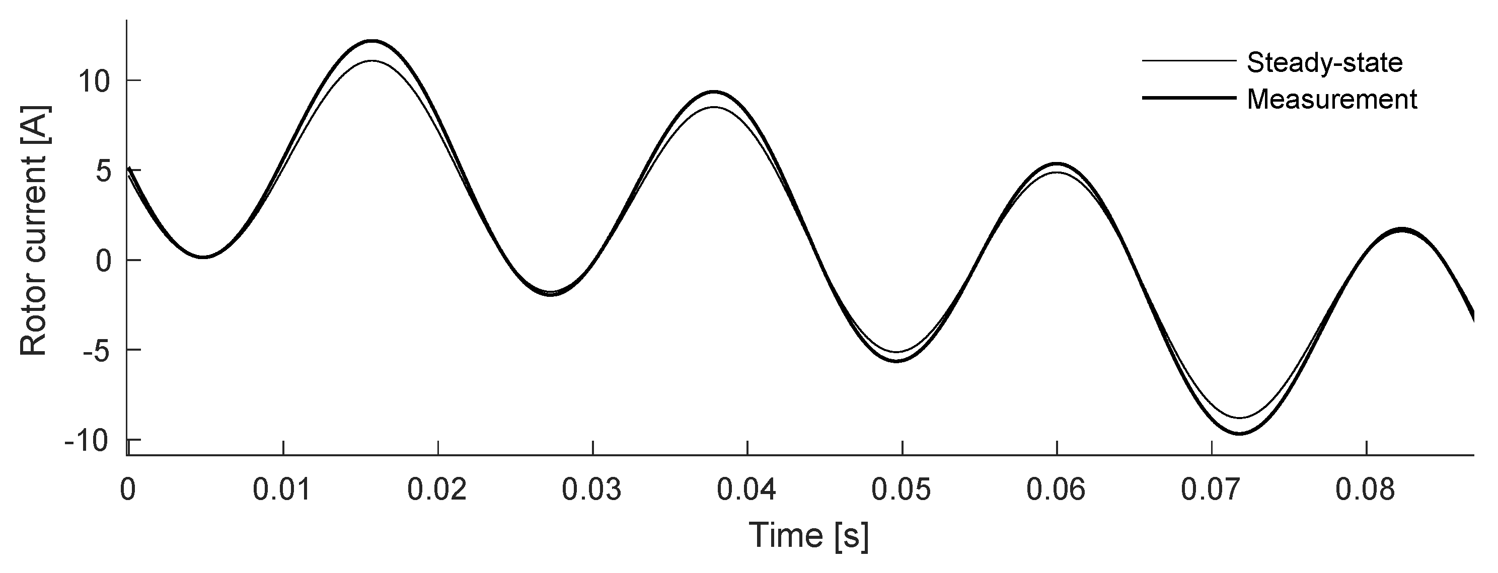
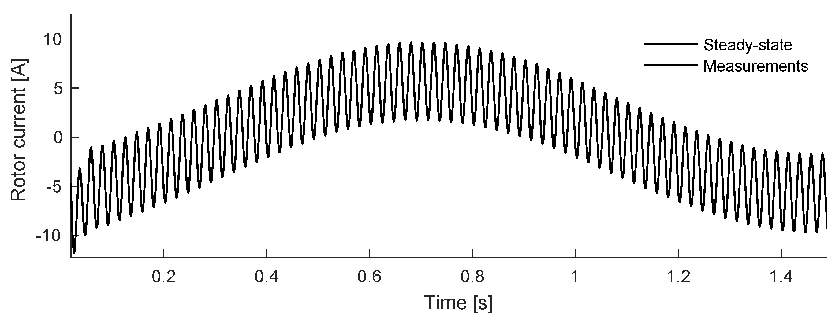
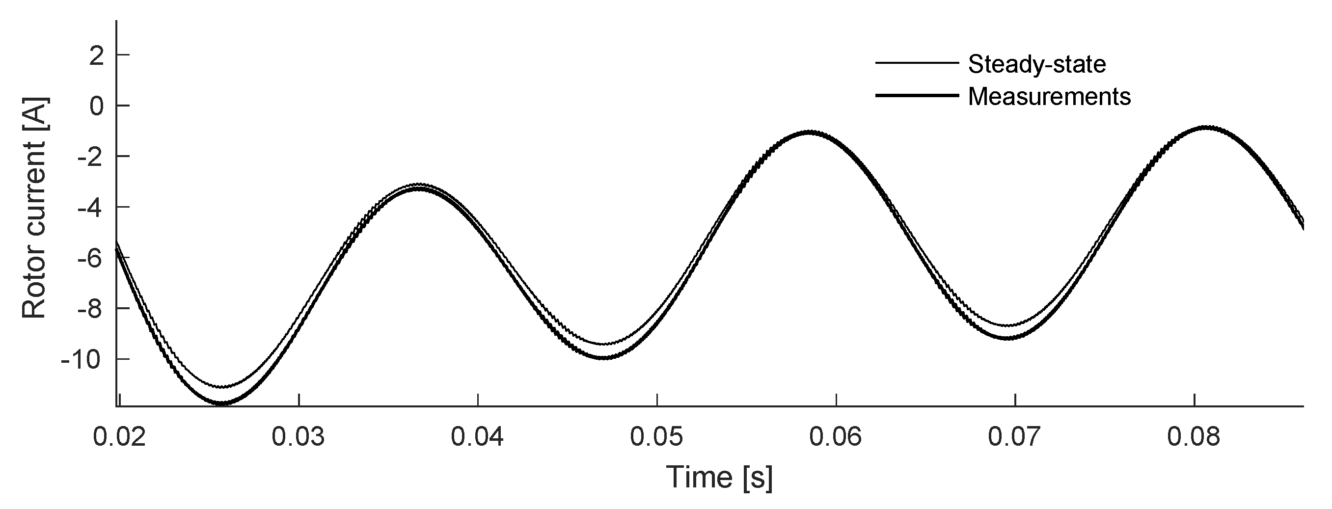
. Figure 25, Figure 26, Figure 27 and Figure 28 show the stator and rotor current waveforms, respectively. Figure 25 and Figure 27 show the results obtained from the proposed model as well as those obtained experimentally. The size of these graphs has been increased to compare the waveforms and verify that their behavior is really similar as shown in Figure 26 and Figure 28.

According to the observed results, SVPWM had a unique feature: it tackled all the major issues related to the SPWM techniques, such as computational complexity, synchronization, total harmonic distortion, DC-link voltage balancing, and common mode voltage. Therefore, this technique is suitable for high-powered applications as it eliminates subharmonics and maintains synchronization, improves THD through various waveform symmetries, and has the advantage of less harmonic content, which is useful in applications that require a low harmonic level for avoiding overheating and malfunction in sensitive systems. In addition, the SVPWM better uses DC-link voltage for the inverter. On the other hand, this switching technique can provide the possibility of obtaining the highest voltage transfer ratio and of optimizing the switching pattern by coordinating the switching state in the rectifier and inverter stages [18].

Finally, when using this switching technique, it was observed that the fluctuation of the inverter input current around its average value was minimized by optimization of the utilized voltage space vectors to reduce the inverter input current harmonics, which extends the lifetime of the DC-link electrolytic capacitors. Experiments with the application of the SVPWM confirmed that the inverter input current harmonics were reduced by up to 5.04% compared to that with the conventional SPWM.

Table 9. Summary of harmonic currents for case study 3.

STATOR CURRENT				ROTOR CURRENT
Seq.	Magnitude	Angle	Freq. (Hz)	Seq.	Magnitude	Angle	Freq. (Hz)
$+$	100%	$-63.9°$	60	$+$	100%	$221.9°$	45
$-$	0.46%	$0.1°$	300	$-$	0.17%	$179.8°$	225
$+$	0.33%	$10.2°$	420	$+$	0.12%	$183.3°$	315
$-$	0.27%	$0.1°$	516	$-$	0.1%	$-$$10.8°$	390
$+$	0.22%	$-$$63.7°$	424	$+$	0.08%	$66.1°$	465
$-$	0.21%	$112.8°$	660	$-$	0.07%	$38.7°$	495
$+$	0.18%	$43.5°$	780	$+$	0.06%	$7.2°$	585
$-$	0.16%	59.1°	876	$-$	0.06%	$-$$180.3°$	750
$+$	0.14%	$-$$119.3°$	1008	$+$	0.05%	$51.6°$	825
$-$	0.14%	$27.7°$	1020	$-$	0.05%	$77.3°$	1035
$+$	0.13%	$87.1°$	1104	$+$	0.04%	$-$$40.1°$	1125
$-$	0.1%	$-$$206.8°$	1356	$-$	0.04%	$88.2°$	1185
$+$	0.1%	$115°$	1380	$+$	0.03%	$-$$31.5°$	1275
$-$	0.09%	$174.2°$	1500	$-$	0.03%	$-$$0.45°$	1320
$+$	0.08%	$92.6°$	1689	$+$	0.02%	$59.3°$	1395
$-$	0.07%	$-$$32.1°$	1740	$-$	0.02%	$60.1°$	1410
$+$	0.06%	$86.9°$	1860	$+$	0.01%	$155°$	1425
${\mathrm{THD}}_{\mathrm{i}}=5.04\%$				${\mathrm{THD}}_{\mathrm{i}}=13.96\%$

presents the global results of the harmonic currents in the DFIG for each winding. It should be noted that the waveforms of the stator and rotor currents presented in this test case were obtained from the harmonic components shown in the table, which were obtained from Equations (10) and (11) mentioned in the previous section.

5.4. Case Study 4: 1.6 MW DFIG-Based Wind Turbine Excited by Nonsinusoidal Voltage in the Rotor Generated by a B2B Power Converter Applying the SVPWM Switching Technique

In order to have a more representative DFIG, in this case study a three-phase induction machine of 1.6 MW was considered. The DFIG parameters are shown in

Table 10. DFIG parameters.

Parameters	1.6 MW-DFIG
Poles number	4 poles
Inertia constant	$63.87 \mathrm{kg}/{\mathrm{m}}^2$
Nominal line current	421 A
Nominal line-to-line voltage	2300 V
Nominal torque	$8900 \mathrm{N}\times \mathrm{m}$
Nominal frequency	60 Hz
$\mathrm{Stator} \mathrm{resistance}, r_s$	0.029 Ω
$\mathrm{Rotor} \mathrm{resistance}, r_r$	0.022 Ω
$\mathrm{Stator} \mathrm{inductance}, L_{ls}$	0.226 mH
$\mathrm{Rotor} \mathrm{inductance}, L_{lr}$	0.226 mH
$\mathrm{Magnetizing} \mathrm{inductance}, L_M$	13.04 mH
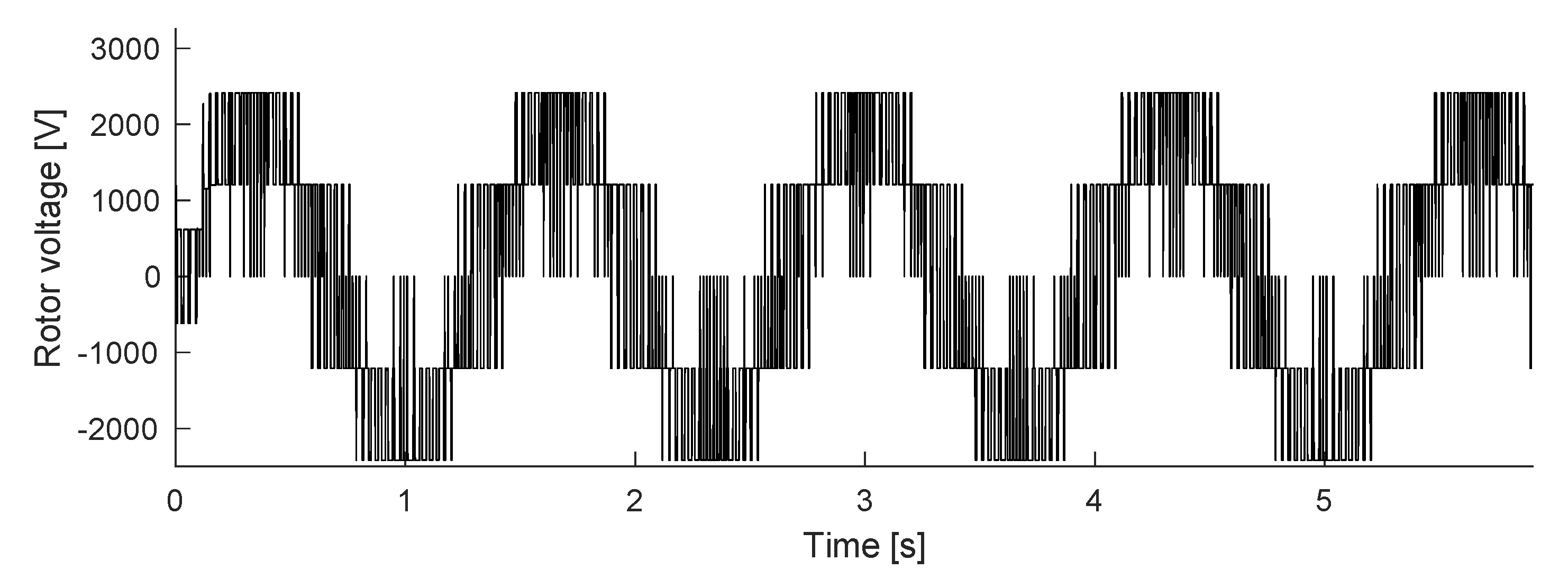
Rotor speed	1500 rpm

. A three-phase balanced voltage source of 2300 V and 60 Hz was applied in the stator, and a three-phase voltage source of 2300 V, 45 Hz was applied in the rotor. The switching technique applied to activate the RSC switches and generate the rotor voltage waveform shown in Figure 29 was SVPWM.

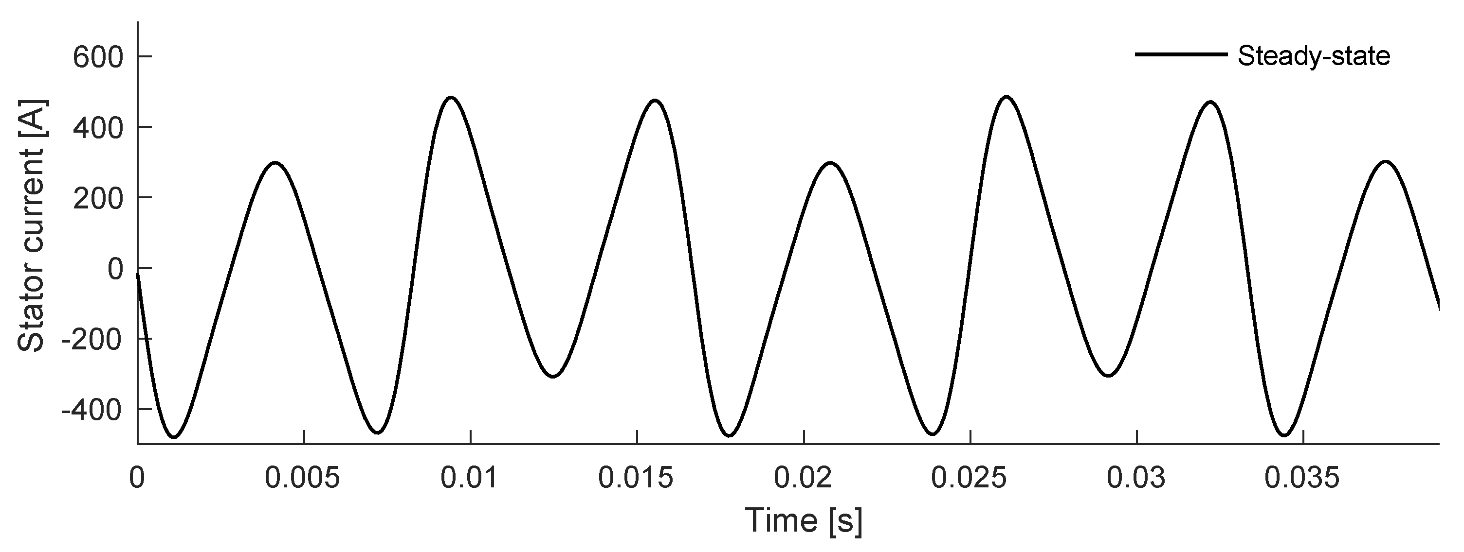
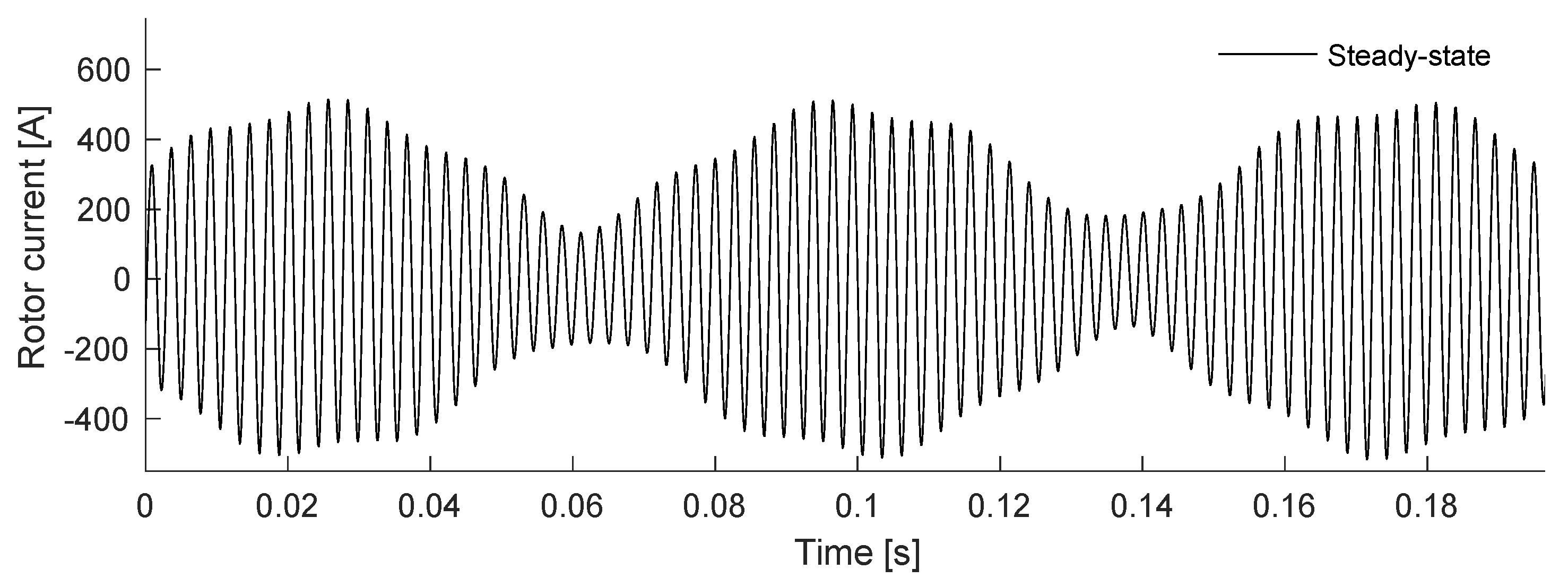
Figure 30 and Figure 31 show the stator and rotor current waveforms, respectively. Both figures show the results obtained from the proposed model in steady-state.

For this case study, the same steady-state model was applied to a 1.6 MW-DFIG equivalent to 2250 HP. It is important to mention that only the simulation results are shown because there is no generator of this capacity in our lab to carry out the relevant experimentation. On the other hand, in the results of this case study, it is clearly visible that the waveforms of both the current in the stator and that of the rotor contained harmonic and interharmonic signals, and this was due to the power of the DFIG, and that at higher power of the generator, the lower the distortion of the currents. Additionally, it was demonstrated that the harmonic voltages generated by the B2B power converter when implementing the SVPWM switching technique had a significant impact on the harmonic emissions of the DFIG and resulted in a range of very high frequency components and interharmonic currents that were slip-dependent. Interharmonic current components for frequencies up to 2 kHz are of special interest in this context.

Table 11. Summary of harmonic currents for case study 4.

STATOR CURRENT				ROTOR CURRENT
Seq.	Magnitude	Angle	Freq. (Hz)	Seq.	Magnitude	Angle	Freq. (Hz)
$+$	100%	$44.5°$	60	$+$	100%	$45.6°$	45
$-$	0.56%	$-17.3°$	300	$-$	0.34%	$-22.1°$	225
$+$	0.51%	$65.8°$	420	$+$	0.31%	$76.4°$	315
$-$	0.48%	$-7.2°$	471	$-$	0.29%	$-98.1°$	332
$+$	0.43%	$-26.3°$	489	$+$	0.23%	$36.2°$	359
$-$	0.39%	$177.4°$	660	$-$	0.12%	$-$$9.7°$	495
$+$	0.33%	$21.6°$	780	$+$	0.11%	$223.1°$	585
$-$	0.28%	$-$$35.3°$	855	$-$	0.1%	$-$$77.9°$	660
$+$	0.22%	$1.2°$	1021	$+$	0.08%	$33.5°$	730
$-$	0.17%	$-9$$3.1°$	1188	$-$	0.08%	$104.2°$	1035
$+$	0.12%	$66.2°$	1290	$+$	0.07%	$100.1°$	1125
$-$	0.09%	$91.9°$	1402	$-$	0.07%	$-$$46.1°$	1174
$+$	0.06%	$-75.6°$	1380	$+$	0.07%	$119.2°$	1203
$-$	0.03%	$22.4°$	1500	$-$	0.06%	$-$$0.45°$	1299
$+$	0.02%	$31.7°$	1677	$+$	0.06%	$59.3°$	1395
$-$	0.01%	$-53.5°$	1789	$-$	0.05%	$-$$56.8°$	1444
$+$	0.01%	$45°$	1890	$+$	0.05%	$7°$	1496
${\mathrm{THD}}_{\mathrm{i}}=7.9\%$				${\mathrm{THD}}_{\mathrm{i}}=18.3\%$

presents the global results of the harmonic currents in the DFIG for each winding.

According to Table 11, for every harmonic voltage, a range of slip dependent interharmonic frequency components will exist in the current spectrum.

The frequencies at which these may appear are related to factors such as operating speed and supply power quality. Additionally, the analysis demonstrated that the harmonic voltages generated by the B2B power converter applying the SVPWM switching technique introduced harmonic components in the stator and rotor current and that, more importantly, they also gave rise to a number of further interharmonic current frequencies whose existence was DFIG design specific. Finally, Figure 32 presents a graphical comparison of the THD levels of the stator and rotor currents when implementing each of the previously mentioned switching techniques.

6. Discussion

In fact, there is no document that compares these three switching techniques together in terms of common results or values in the literature. Therefore, in this section the authors discuss the results and their interpretation from the perspective of previous studies and the hypothesis of the work, as well as highlight the future directions of this research.

In this paper, a 3-kW DFIG is modeled, simulated, and validated in a MATLAB-Simulink^® environment. To connect the DFIG to the electrical grid, a B2B power converter is used interconnected to the rotor winding with the electrical grid, where harmonic distortion is produced in both the stator and rotor currents of the DFIG. Therefore, the waveforms of these currents are investigated and improved from a power quality point of view using various types of switching techniques, including carrier-based PWM compared with a triangle waveform and a sine wave (SPWM), a third harmonic injection carrier-based PWM (THIPWM), and a space vector modulation (SVM). In comparison with the simple PWM technique, SPWM, THIPWM, and SVM switching techniques have many advantages, such as lower THD, minimal number of switching losses, and increased output fundamental voltage. All these techniques are compared from the point of view of power quality, taking into account the limits of the IEEE 519 standard.

It is worth mentioning that this study showed that the proposed approach using THIPWM or SVPWM resulted in a superior performance in terms of THD in all modes of operating conditions and a reduction in complexity and cost of the system:

• The SPWM switching technique cannot use the full voltage of supply in the inverter and has high harmonic distortion in the produced waveform of output voltages because the SPWM characteristics of switching are not of a symmetrical nature.
• The THIPWM switching technique has many features, as the reduction in the losses of commutation, greater modulation index amplitude, higher utilization of the DC-link voltage, and a reduction in the THD of the waveform of output voltages, compared with the SPWM technique lead to better reliability and electrical performance. Therefore, Third Harmonic Injection PWM is preferred in a three-phase application because the third harmonic component will not be introduced in three-phase systems. The THIPWM is better in the utilization of a DC source.
• The results obtained with the SVPWM switching technique show a considerable reduction in THD compared with SPWM for all parameters (inverter voltage, the stator currents, and even for active and reactive power). The SVPWM brings some drawbacks to controllers, however, such as the compromised output current because of the back EMF disturbance and nonlinearity of the system, as well as the lack of inherent overcurrent protection, etc.

As such, the SVPWM and THIPWM offer the same advantages as the SPWM schemes. The simple and direct implementation of THIPWM, however, gives it advantage over the SVPWM: there is no need to track the operating sector or add a state machine for switch sequencing of THIPWM. In terms of harmonic distortion, high switching frequency THIPWM makes it appropriate for harmonic distortion elimination.

7. Conclusions

This paper presented the model of a DFIG in a steady-state connected to the electrical grid by means of a B2B power converter, which was implemented with different switching techniques for harmonic propagation studies. The implemented PWM switching techniques are SPWM, THIPWM, and SVPWM for analyzing the harmonic content of the stator and rotor currents at an established average wind speed. The following are obtained from this study.

• When the rotor of the DFIG is excited with a nonsinusoidal voltage generated by the B2B power converter, harmonic and interharmonic currents are generated in the stator and rotor of the machine. Under such conditions, the appearance of harmonic and interharmonic currents in the stator of a DFIG requires a controller included in the RSC control system.
• The harmonic stator current generation is clearly diminished with increasing rotor speed (i.e., increasing wind speed). This effect is more serious in the case of an unbalanced stator voltage, since the harmonic components and the negative sequence fundamental component always have gains greater than 1.
• For rotor speeds close to nominal speed, where the fundamental rotor voltage is small, the THD becomes very high; the worst condition occurs at synchronous speed where the fundamental voltage is 0.
• The stator and rotor currents of the DFIG connected to the electrical grid coincide with those obtained by means of the experimental prototype, both in magnitude and in phase angle.
• The THD index, both voltage and current, improves with varying switching techniques; the reduction in THD is significant in all tests.

Finally, this paper offers a clear analysis of the harmonic frequencies generated by the DFIG when excited by a B2B power converter to which different switching techniques have been applied, resulting in an appropriate model for the harmonic and interharmonic analysis of the DFIG, which can be used in power systems.