Ultra-Short Window Length and Feature Importance Analysis for Cognitive Load Detection from Wearable Sensors

Abstract

Human cognitive capabilities are under constant pressure in the modern information society. Cognitive load detection would be beneficial in several applications of human–computer interaction, including attention management and user interface adaptation. However, current research into accurate and real-time biosignal-based cognitive load detection lacks understanding of the optimal and minimal window length in data segmentation which would allow for more timely, continuous state detection. This study presents a comparative analysis of ultra-short (30 s or less) window lengths in cognitive load detection with a wearable device. Heart rate, heart rate variability, galvanic skin response, and skin temperature features are extracted at six different window lengths and used to train an Extreme Gradient Boosting classifier to detect between cognitive load and rest. A 25 s window showed the highest accury (67.6%), which is similar to earlier studies using the same dataset. Overall, model accuracy tended to decrease as the window length decreased, and lowest performance (60.0%) was observed with a 5 s window. The contribution of different physiological features to the classification performance and the most useful features that react in short windows are also discussed. The analysis provides a promising basis for future real-time applications with wearable sensors.

1. Introduction

In the near future, unobtrusive, reliable, and affordable wearable sensors will enable cognitive state estimation of a person in real-time. The cognitive state, i.e., a person’s overall capacity and readiness to meet everyday situations, is affected by various conditions such as sleep deprivation [1,2], acute stress [3,4], and cognitive load [5] and thus cognitive state estimation would be beneficial in many application areas, e.g., transportation, industry, rehabilitation, and education.

In many working environments, the modern technology such as human computer interaction (HCI) systems impose high cognitive demands for humans, thus increasing the cognitive load of a person [6]. Real-time assessment of a person’s cognitive load could be used to identify overload situations where the probability of error is increased. Further, in the near future, HCI and cyber-physical systems could use the information to optimize user interface content and interactions to match the imposing workload with the prevailing cognitive capacity of the user. However, this would require seamless operation between the HCI system and the users, meaning accurate and real-time (with minimal delay) assessment of the cognitive load.

Humans respond to external stimuli by adjusting nervous system functions, which causes physiological reactions that can be detected from different type of biosignals. The autonomic nervous system (ANS) is one of the major neural pathways activated by stress [7]: the sympathetic branch of the ANS prepares body for an emergency while the parasympathetic branch facilitates recovery [8]. An increase in the heart rate (HR) reflects the sympathetic nervous system (SNS) activation while parameters derived from the heart rate variability (HRV) parameters can capture variations both in the SNS and parasympathetic nervous system (PNS) activations [9]. Galvanic skin response (GSR) reflects the activity in the sweat glands, which are solely connected to the SNS. Therefore, the GSR is considered to be an undisturbed measure of SNS activation [8]. In addition, in acute stress the SNS triggers peripheral vasoconstriction which reduces the flow in the blood vessels and reduces the skin temperature (ST) [10]. However, the after a short delay the blood flow recovers resulting in delayed skin warming [9,11,12].

The changes in the cognitive load are also reflected in various biosignals that can be measured by using biosensors, e.g., wearable devices [13,14]. For instance, increasing task difficulty (or cognitive load) and acute stress increases the HR and breathing rate [15], ST [11] as well as GSR [16] and decreases the HRV [17], number of eye movements [18], and increases the blink rate [19,20].

Real-time cognitive load estimation means processing a stream of biosignals with minimal latency. Research on affective, or cognitive state/load, detection systems has focused mainly on state recognition methodology and optimizing the used sensor set (see, e.g., [21]). To achieve real-time or continuous monitoring of the cognitive state/load, the segmentation part (i.e., selection of used window length) of the state detection pipeline has received little attention and it requires further research.

The cognitive load is estimated from various biosignals and each of these signals has its own characteristics. For instance, HR could be considered as a periodic signal, whereas some other biosignals, such as eye movements and GSR reactivity, have a bursty nature and are more linked to the stimulus or task at hand. Further, the level of some slow-acting signals, skin temperature and the tonic component of the GSR signal, may increase or decrease during a cognitive load (e.g., due to changes in alertness). Thus, the varying nature of the biosignals sets limits to the window lengths: the length must be long enough to include sufficient variation and periods for the periodic signals but short enough that bursty events do not average out.

In recent studies the window lengths have varied (see

Table 1. Previous studies in the affective computing domain with an emphasis on state detection based on physiological variables conducted mostly in constrained or laboratory environments.

Study	Signals (Sampling Rate in Hz)	Window Lengths Used	Overlap	Optimal Window Length	Model	Classification Performance
Cognitive state detection
[9]	GSR (1000), ST (1000), HRV **	30–300 s	0–90%	30 s/60 s	LDA, kNN, QDA, SVM	97% accuracy (binary)
[14]	ST (1), GSR (1), HR (1), HRV (1)	30 s	-	-	Bagging, XGB	68% and 82% accuracy (binary, two datasets)
[23]	EOG (250)	1–10 s	-	10 s	LDA	87% accuracy (binary)
[20]	HR **, HRV **, EOG (1000)	45 s	15 s	-	XGB, SVM	86% accuracy (three classes) 97% accuracy (binary)
Stress detection
[24]	ST (4), GSR (4), HR (1), HRV *	30–360 s	5–275 s	300 s	SVM	73% accuracy (three classes)
[25]	ST (32), GSR (32), HR **, HRV **, RESP (32)	30 s	29 s	-	dBN	85% mean of sensitivity and specificity (binary)
[26]	HRV **	30–300 s	-	300 s	kNN	94% accuracy
[27]	GSR (32), HRV **	50 s	30 s	-	SOM	79% mean of sensitivity and specificity (binary)
Emotion detection
[28]${}^F$	ACC (NA), GSR (4), HR (NA)	60–300 s	-	-	DT, BN	51% error rate on detecting arousal
[29]	EEG (256), HRV **	90 s	-	-	SVM	75% and 82% accuracy (valence and arousal, binary)
[30]	HRV **	90 s	-	-	SVM	71% accuracy (positive or negative emotion)
[31]	EEG (256)	1 s	-	-	LDA	73% accuracy (positive or negative emotion)
Stress / emotion detection
[32]	ACC (32), ST (4), GSR (4), HR (1), HRV *	15–120 s	0.25 s window slide	120 s	LDA	84% accuracy (binary)
[33]	ACC (32), ST (4), GSR (4), HR (1), HRV *	60 s	0.25 s window slide	-	RF	76% accuracy (three classes) 88% accuracy (binary)
Odor pleasantness classification
[34]	EEG (250), HRV **	6 s	-	-	LDA	0.46 Cohen’s kappa

${}^F$ Field study. * Interbeat intervals used to derive HRV were obtained on-device from blood volume pulse signal sampled at 64 Hz; ** Interbeat intervals used to derive HR/HRV were obtained from an electrocardiogram sampled at 200 Hz [30], 250 Hz [34], 256 Hz [25,27,29], and 1000 Hz [9,20]. Abbreviations: ACC: acceleration, (d)BN: (dynamic) Bayesian network, DT: decision tree, EEG: electroencephalogram, EOG: electro-oculogram, GSR: galvanic skin response, HR: heart rate, HRV: heart rate variability, kNN: k-nearest neighbors, LDA: linear discriminant analysis, NA: not available, QDA: quadratic discriminant analysis, RESP: respiration, RF: random forest, SOM: self-organizing map, ST: skin temperature, SVM: support vector machine, XGB: extreme gradient boosting.

) from 1 s to 360 s. In most studies, the window lengths have been selected based on the physiology, task duration, or previous studies. However, the literature on ultra-short windows (<60 s, especially <30 s), e.g., in HR and HRV analyses is rather limited (see the review by Shaffer and Ginsberg [22]) and therefore, there may not be theoretical limits for the physiological features used in real-time/continuous cognitive state estimation. In addition, there are few studies where the effect of window length to classification accuracy has been studied (see Table 1) and even those have mainly used windows with length of 30 s or more.

Healey et al. [28] attempted emotion detection in a field study in windows of 60 s, 180 s, and 300 s, but the best window length was not reported since each one showed poor performance. Gjoreski et al. [24] experimented with window lengths between 30 s and 360 s in a laboratory study of stress detection, and selected the 300 s window for a continuation study with field data. Anusha et al. [9] found that a 30 s window performed the best for ST, and a 60 s window for GSR in cognitive state detection; however, window length experiments were not conducted for HRV. Marshall [23] detected the cognitive state based on eye movements and found that a 10 s window provided highest detection accuracy. Siirtola [32] studied stress detection in a laboratory with window lengths between 15 s and 120 s. It was found that whereas the 120 s window performed the best, a 15 s window performed better than a 30 s window and almost the same as a 60 s window, which shows that window lengths shorter than 30 s have the potential to perform well despite containing less data than longer windows.

In a related context, Kroupi et al. [34] detected odor pleasantness in 6 s windows based on electroencephalogram and HRV measurements. Moreover, Kreibig [8] reports on multiple studies using shorter than 30 s averaging periods for physiological responses. However, the goal in those studies was to observe the effects emotions have on functions of the autonomous nervous system, rather than classifying between emotional/cognitive states based on those effects.

Thus, the existing research on cognitive state recognition has not focused on the segmentation part of the state detection pipeline. Even when experiments with different window lengths have been conducted, they have focused on rather long window lengths, despite the fact that shorter window lengths have been considered in related contexts. The novelty in this study is on performing a systematic comparison of ultra-short windows (30 s or less) in terms of the classification performance for cognitive load detection. An analysis of the contribution of different features is also presented, and the variation of the most useful features between tasks is discussed. Further, individual differences related to the optimal window length and feature variation between the study subjects as well as the effect of optimizing classifier hyperparameters are studied.

2. Materials & Methods

2.1. Dataset

The CogLoad dataset from [14] was used in this study. The dataset includes 23 participants (7 females, mean age 29.5 years with a standard deviation of 10.1 years) who solved cognitive tasks of varying difficulty. In the first part, the participants solved N-back tasks, i.e., 2-back and 3-back tasks, with a three-minute rest after each of them, and answered questions to determine their personality. In the second part, six elementary cognitive tasks (ECT) each with three difficulty levels were presented: the Gestalt Completion test (GC), the Hidden Pattern test (HP), Finding A’s test (FA), Number Comparison test (NC), Pursuit test (PT), and Scattered X’s test (SX), with a rest period between them. After each task, the participants were asked to fill in the NASA-TLX questionnaire to determine their subjective cognitive load, however, those questionnaires were not utilized here. Further details on the study protocol and tasks can be found in [14].

While doing the tasks, the participants’ physiological response was measured with a wrist device (Microsoft Band). The measurements included the HR, R-to-R intervals (RR), GSR, ST and 3-axis acceleration, which was not used in this study. The open-sourced dataset contains the data re-sampled to a frequency of 1 Hz. However, the HR and RR were derived on-device from an optical sensor and the raw measurements used to obtain those two signals were not available. Thus, the rate at which the HR and RR were measured was truly not constant but dynamic, and depended on when the heartbeats occurred.

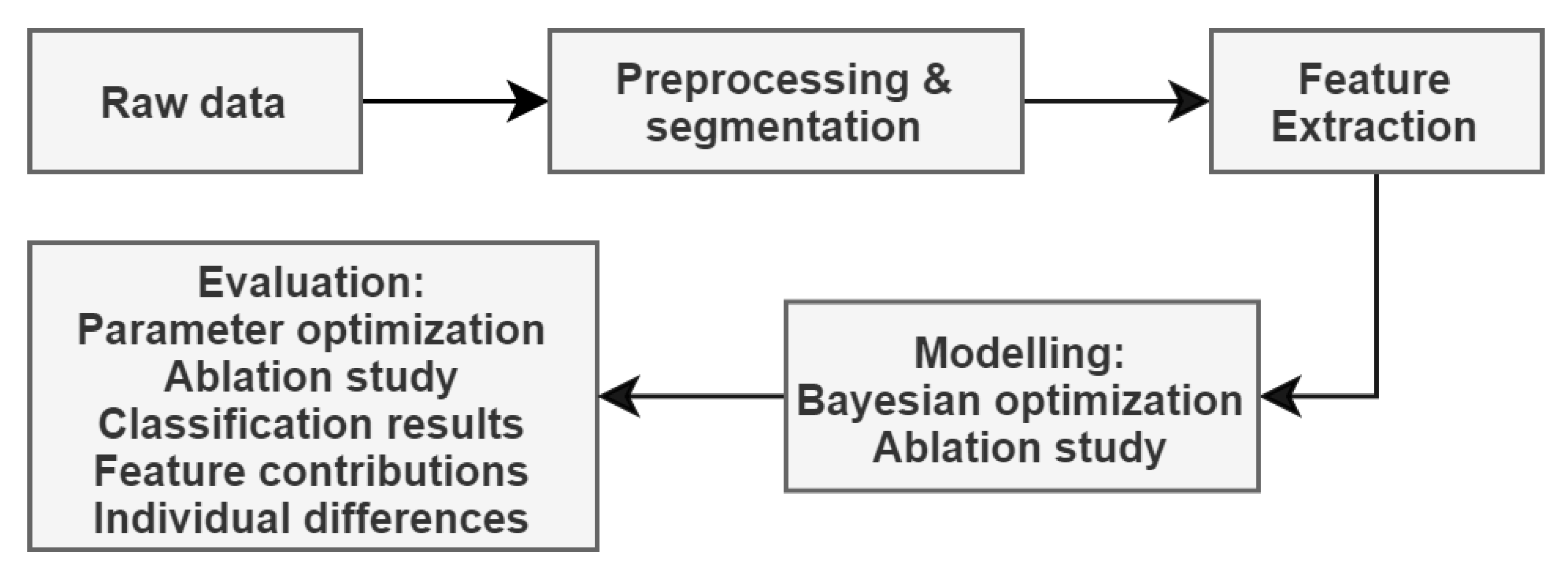
Figure 1 depicts the steps taken in analyzing the dataset and evaluating the results.

2.2. Data Preprocessing, Segmentation and Feature Extraction

The main focus in this study was on evaluating the classification performance of cognitive load at different window lengths of less than 30 s in duration. Window lengths selected were 5 s, 10 s, 15 s, 20 s, 25 s, and 30 s in duration, and a 50% window overlap was employed to increase the amount of data.

The time taken by the participants to complete the tasks varied between 18 s and 190 s. If a task lasted for a shorter time than window length, that single task was removed from the experiment with the specific window length to make sure that a shorter actual task length would not skew the results; approximately 4% of all tasks were completed in less than 30 s. In addition, it was noted that sometimes the data had been filled by carrying the last observation forward, i.e., a signal was constant for a period of time. As many features could not be calculated if there was not enough variation, segments with less than 25% unique values in the RR-, HR-, or GSR-signal were removed.

Next, features were extracted at each window length. According to [21,35], features that are usually extracted from the signals used here contain the statistics of each signal, heart rate variability from the RR-signal, and skin conductance response analysis for the GSR signal.

In this study, the statistical features of the RR, HR, GSR, and ST and their first and second derivatives were computed. The statistical features included the mean, standard deviation, minimum, maximum, difference between minimum and maximum, lower and upper quartile, interquartile range, and coefficient of variation.

A skin conductance response (SCR) analysis was conducted for the GSR signal to extract additional features. Like in the original paper using the same dataset [14], the signal was first preprocessed with a sliding mean filter, and then fast-acting (phasic) and slow-acting (tonic) components were extracted. Normally, the SCR analysis is used especially to extract features from the phasic component and SCR peaks [21,35]. In this analysis, however, it often happened that a segment did not contain any SCR peaks, especially with shorter window lengths. Therefore, the features extracted from the phasic component included the number of SCR peaks and the statistics (mean, standard deviation, median, lower and upper quartile, minimum and maximum) of its first and second derivative, and the total time the first derivative of the phasic component was positive (rise-time) and negative (descend-time). The features extracted from the tonic component included its mean, standard deviation, minimum, maximum, ratio of maximum and minimum, and its correlation with time.

Additionally, heart rate variability (HRV) features were extracted from the R-to-R intervals. Following [22,36], the HRV features extracted included the mean, median, and range of normal-to-normal intervals, standard deviation of normal-to-normal intervals (SDNN) and successive differences, percentage and number of normal-to-normal intervals differing by more than 20 ms and 50 ms, root mean square of successive differences (RMSSD), ratio of SDNN and mean normal-to-normal intervals (CVNNI), ratio of RMSSD and mean normal-to-normal intervals (CVSD), power in very low, low and high frequency bands, total power, ratio of low and high frequency power, normalised low and high frequency power, triangular index, (modified) cardiac sympathetic index, cardiac vagal index, and Poincaré plot indices SD1, SD2, and SD1/SD2.

A total of 157 features were extracted and they are listed in

Table 2. List of computed features. Abbreviations used later in text and in figures are in parenthesis.

Category	Features
Statistical features for each signal (d0) and their first (d1) and second (d2) derivatives	mean, standard deviation (std), minimum (min), maximum (max), difference between minimum and maximum (range), lower (lq) and upper quartile (uq), interquartile range (iqr), and coefficient of variation (cv)
Heart rate variability (HRV)	mean, median, and range of normal-to-normal intervals (mean, median, range nni), standard deviation of normal-to-normal intervals (sdnn) and successive difference (sdsd), root mean square of successive differences (rmssd), ratio of sdnn and mean nni (cvnni), ratio of rmssd and mean nni (cvsd), signal power in very low (vlf), low (lf), and high (hf) frequency bands, total power, ratio of lf and hf, normalised lf and hf (lfnu, hfnu), triangular index, cardiac sympathetic index (csi), modified csi, cardiac vagal index (cvi), and Poincaré plot features (SD1, SD2, ratio of SD1 and SD2)
Skin conductance response (SCR)	phasic component: number of peaks (npeaks), time first derivative was positive (risetime) and negative (dectime), and mean, std, median, lq, and uq of first (diff1) and second (diff2) derivatives tonic component (scl): mean, std, min, max, ratio of max and min (slope), and its correlation with time (corrwithtime)

. Afterwards, a sanity check was conducted for the features computed. Some features had a significant amount of missing or infinite values, or showed little variation. Thus, features with missing values, infinite values, or variance below 0.01 were removed for each window length. The number of remaining features was 93 at window lengths from 20 s to 30 s, 91 at window lengths of 10 s and 15 s, and 82 at a window length of 5 s.

According to the criteria stated above, features that were removed most often were the HRV parameters CVSD and CVNNI, coefficient of variation of the HR and its derivatives, statistical features of the derivatives of the phasic component of the GSR signal, standard deviation of the tonic component of the GSR signal, and statistical features of the derivatives of the ST signal across the different window lengths. Additionally, several HRV parameters were removed from the shortest window length.

The features were normalized using within-subject standardization, meaning that each feature was transformed by subtracting its mean and dividing by its standard deviation separately for each participant. Person-specific standardization was conducted instead of person-independent standardization, since it has shown improved performance in earlier work in similar contexts [14,20,37].

2.3. Model and Experimental Protocol

The classification task was formulated as binary classification between a cognitive load and a rest class. All data segments during a cognitive task (N-back task or one of the six ECTs) were annotated as a cognitive load, and all the rest periods were annotated as rests. The segments during which the participant answered the questionnaires were removed from the data. The number of instances in both classes at each window length are reported in

Table 3. Number of instances in cognitive load and rest classes at each window length.

	30 s	25 s	20 s	15 s	10 s	5 s
Cognitive load	1654	2110	2840	4055	6336	12,763
Rest	1406	1791	2407	3437	5393	10,937

. Because the number of samples in each class is reasonably balanced (approximately 46% rests and 54% cognitive loads for each window length), the classification performance was assessed in terms of accuracy, the percentage of correctly classified samples.

Extreme Gradient Boosting [38] (XGB) was selected as the classification model for the following reasons: the classifiers from the random forest family and the boosting method have been shown to be strong classifiers [39], XGB has shown good performance earlier in similar contexts [14,20] and because XGB is computationally efficient and scales to very large datasets [38]. XGB is an ensemble of decision trees, each of which splits the data hierarchically, aiming to contain data originating from a single class in each leaf node. XGB uses the gradient descent algorithm to construct the trees sequentially so that each subsequent tree attempts to fix the errors made by preceding trees.

Specifically, XGB aims to minimize the regularized objective function

$$\mathcal{L}\left(\widehat{y}\right)=\sum _{i=1}^{n}l({\widehat{y}}_i,y_i)+\sum _{k=1}^K\Omega \left(f_k\right),$$

(1)

where $\Omega \left(f\right)=\gamma T+\frac{1}{2}{\lambda \left|\right|w\left|\right|}^2$. Here, n is the number of observations, l is a differentiable convex loss function measuring the difference between the prediction ${\widehat{y}}_i$ and the target $y_i$, K is the number of classification trees, $f_k$ are classification tree functions, $\Omega$ is a regularization function penalizing the complexity of the model, T is the number of leaves in a tree, $\gamma$ and $\lambda$ are regularization parameters and w are leaf weights. Assume that $I_L$ and $I_R$ are the instance sets of left and right nodes after a split. Then, letting $I=I_L\cup I_R$, the loss reduction after the split is given by

$${\mathcal{L}}_{split}=\frac{1}{2}\left[\frac{{\left({\sum }_{i\in I_L}{g}_i\right)}^2}{{\sum }_{i\in I_L}{h}_i+\lambda }+\frac{{\left({\sum }_{i\in I_R}{g}_i\right)}^2}{{\sum }_{i\in I_R}{h}_i+\lambda }-\frac{{\left({\sum }_{i\in I}{g}_i\right)}^2}{{\sum }_{i\in I}{h}_i+\lambda }\right]-\gamma ,$$

(2)

where $g_i={\partial }_{{\widehat{y}}^{(t-1)}}l(y_i,{\widehat{y}}^{(t-1)})$ and $h_i={\partial }_{{\widehat{y}}^{(t-1)}}^{2}l(y_i,{\widehat{y}}^{(t-1)})$ are the first and the second order gradient statistics of the loss function at the t-th iteration. In practice, the formula above is used for evaluating the split candidates, and the splits are found either with an exact or approximate greedy algorithm that are implemented in [38]. So, at each boosting iteration t, a classification tree $f_t$ whose splits are found using a greedy algorithm with Equation (2) and that most improves the model according to Equation (1) is added to the model.

The performance of the XGB model depends on its hyperparameters that describe the structure of each tree and that affect the convergence of the loss function. The hyperparameters were optimized using Bayesian optimization (see Section 2.4) but an ablation study using default hyperparameters was also conducted. The following hyperparameters were optimized:

• max_depth: the maximum depth of each tree
• n_estimators: the number of estimators in the model
• reg_alpha: L1 regularization term
• reg_lambda: L2 regularization term
• subsample: the ratio training instances used for each boosting iteration
• learning_rate: the step size shrinkage used in each update to prevent overfitting
• gamma: the minimum loss reduction required to make a further split on a leaf node of the tree
• colsample_bytree: the ratio of the number of features used to create each tree
• colsample_bynode: the ratio of the number of features used at each node (split)
• colsample_bylevel: the ratio of the number of features used at each tree level

The dataset was published with participants divided into training and testing sets, with 18 subjects for training and 5 for testing. However, the ablation study without Bayesian optimization showed significantly higher performance for the test subjects than the training subjects even though the model had not seen the data of the test subjects. Therefore, test subjects’ data appeared to be different from the data of the training subjects. So, instead of using the fixed train-test-split the dataset came with, it was decided to use cross-validation with both the training and testing subjects in a single pool to validate the modelling results with Bayesian optimization. Individual differences are further elaborated in Section 3.4.

In general, leave-one-subject-out (LOSO) validation is recommended in the affective computing domain [21], meaning that each subject is left out in turn for testing and the rest of the data is used for training the model. Moreover, when tuning hyperparameters, an internal validation with training data is required to make sure that the best hyperparameters are selected according to the validation performance, and not the testing performance.

Instead of LOSO validation, it was decided to use the leave-two-subjects-out (LTSO) validation method when tuning hyperparameters because the process is computationally intensive, especially since it had to be completed for each window size separately, and because the number of participants in the dataset was relatively large (LOSO validation would correspond to 23-fold cross-validation). So, each hyperparameter configuration was evaluated with data of two randomly selected subjects left out for testing, with internal leave-two-subjects-out validation to select the hyperparameters. This had the effect of approximately halving the computation time during the Bayesian optimization compared to using LOSO validation. However, to comply with earlier research the final results are also reported with LOSO validation for the best hyperparameter configuration.

2.4. Hyperparameter Optimization

Bayesian optimization is a derivative-free search strategy for the global optimization of functions that are expensive to evaluate. The algorithm starts by setting a prior distribution over the parameters to optimize and evaluating the function (here, a function value refers to LTSO validation accuracy with the XGB model) a certain number of times on parameter values sampled from the prior distribution. Then, for a set number of iterations, posterior distributions of each parameter over the function are updated using all the available data, the values maximizing an acquisition function over the current posteriors are sampled, and the function is evaluated using those values. For more details on the algorithm we refer to [40].

Table 4. Hyperparameters optimized for the XGB model, and their prior distributions using the hyperopt syntax.

Hyperparameter	Prior
max_depth	hp.quniform(’max_depth-xg’, 2, 12, 1)
n_estimators	hp.quniform(’n_estimators-xg’, 20, 250, 10)
reg_alpha	hp.uniform(’reg_alpha-xg’, 0, 1)
reg_lambda	hp.uniform(’reg_lambda-xg’, 0, 1)
subsample	hp.choice(’subsample’, [1, hp.uniform(’subsample-xg’, 0.7, 1)])
learning_rate	hp.uniform(’learning_rate-xg’, 0.01, 0.5)
gamma	hp.choice(’gamma’, [0, hp.uniform(’gamma-xg’, 0, 0.05)])
colsample_bytree	hp.choice(’colsample_bytree’, [1, hp.uniform(’colsample_bytree-xg’, 0.7, 1)])
colsample_bynode	hp.choice(’colsample_bynode’, [1, hp.uniform(’colsample_bynode-xg’, 0.7, 1)])
colsample_bylevel	hp.choice(’colsample_bylevel’, [1, hp.uniform(’colsample_bylevel-xg’, 0.7, 1)])

lists the hyperparameters that were optimized and the priors used for each parameter. Overall, non-informative priors were employed, and the prior distributions were either discrete uniform distributions on a given interval and step size (parameters max_depth and n_estimators), continuous uniform distributions on a given interval (parameters reg_alpha, reg_lambda, and learning_rate), or a random choice between a constant or a number sampled from a continuous uniform distribution on a given interval (parameters subsample, gamma, colsample_bytree, colsample_bynode, and colsample_bylevel).

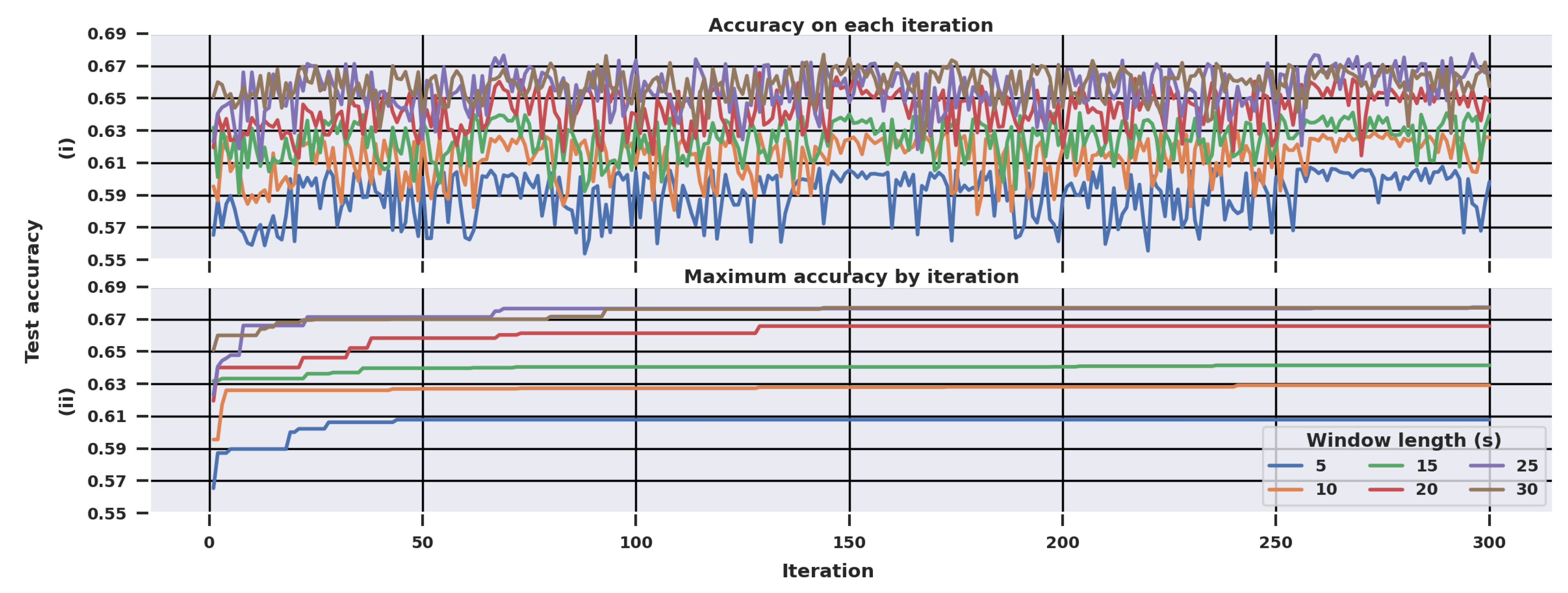
Optimization was continued for a total of 300 iterations at each window length. The number of iterations was selected experimentally. As seen in Section 3.1, the performance improved little after 100–150 iterations. Thus, the procedure was continued for twice that long since it would have been unlikely that scores would improve much after that.

2.5. Statistical Tests

Statistical tests were conducted to determine (1) whether there was a statistically significant difference in the classification performance between the different window lengths, and (2) whether hyperparameter optimization provided statistically significantly more accurate classification (effect of ablating Bayesian optimization). First, subject-by-subject accuracy was obtained for each subject by training the model with all the other subjects in training data. Then, paired t-tests were employed for both scenarios. Pairs were formed from the accuracies observed for each subject at (1) two different window lengths and (2) for optimized and default hyperparameters. A t-test was selected since the subject-by-subject accuracies were normally distributed. In all tests, the Benjamini-Hochberg correction was used to control the false discovery rate, with probability of type I error set to 0.05.

2.6. Computational Tools

The analysis was completed using the Python programming language. The libraries employed were scikit-learn (preprocessing and cross-validation implementation) [41], xgboost (implementation of XGB model) [38], hrv-analysis (calculating HRV features) [42], neurokit2 (signal processing and SCR analysis) [43], and hyperopt (Bayesian optimization) [44].

3. Results

3.1. Parameter Optimization

Figure 2 shows the evolution of the hyperparameter optimization. It is evident from the figure that most improvement took place within the first one hundred iterations for each window length, with only minor improvements afterwards. Overall, 30 s and 25 s window lengths performed similarly, and the accuracy decreased as the window length decreased further.

Figure 3 displays the posterior distributions of the max_depth parameter which describes the depth of each tree in the XGB model. The distribution of each window length is similar to the Gamma distribution truncated between 2 and 12 (since the prior was truncated between 2 and 12). Most of the probability mass was located between the depths from 2 to 6, and the best value found (black vertical lines) are located at depths 2 and 3 for all window lengths except for 25 s, which achieved its best performance at a maximum depth of 6.

Similar figures of posterior distributions for the rest of the hyperparameters are available as supplementary material, together with a table of all the tested hyperparameter configurations and their performance for each window length.

3.2. Classification Results

Table 5. The classification accuracy (%) for each window length, with leave-two-out validation with optimized parameters (LTSOopt), and leave-one-out validation with optimized parameters (LOSOopt) and default model parameters (LOSOdef). Standard deviations in parenthesis.

	30 s	25 s	20 s	15 s	10 s	5 s
LTSOopt	66.9 (4.9)	67.4 (4.5)	66.1 (5.2)	64.1 (4.1)	62.6 (4.3)	60.8 (3.5)
LOSOopt	67.2 (9.0)	67.6 (8.6)	65.4 (8.0)	63.6 (7.7)	62.2 (7.6)	60.0 (6.4)
LOSOdef	65.0 (7.5)	64.5 (8.3)	63.5 (6.6)	60.1 (6.6)	58.5 (6.5)	56.4 (5.7)

presents the classification accuracies obtained for each window length with the LTSO validation used during the Bayesian optimization, and with the LOSO validation with optimized and default model parameters. The results for statistical tests for the performance with default and optimized hyperparameters, and the different window lengths, are shown in

Table 6. Results for the Benjamini-Hochberg corrected paired t-tests between the default and optimized hyperparameters with LOSO validation.

30 s		25 s		20 s		15 s		10 s		5 s
t	p	t	p	t	p	t	p	t	p	t	p
−2.40	0.03	−4.13	<0.001	−2.62	0.02	−3.63	<0.001	−5.09	<0.001	−6.12	<0.001

and

Table 7. Results for the Benjamini-Hochberg corrected paired t-tests between accuracies for different window lengths.

	30 s		25 s		20 s		15 s		10 s
	t	p	t	p	t	p	t	p	t	p
25 s	−0.64	0.53
20 s	1.95	0.07	2.38	0.03
15 s	3.48	0.003	3.82	0.002	3.25	0.005
10 s	4.2	0.001	4.26	0.001	4.78	<0.001	3.3	0.004
5 s	5.58	<0.001	5.69	< 0.001	7.19	<0.001	6.92	<0.001	5.84	<0.001

, respectively.

There were no differences in the mean classification performance between the LTSO and LOSO validation strategies (less than 1% difference at each window length), but LTSO validation seemed to underestimate standard deviations compared to LOSO validation. Since standard deviations were calculated from the overall accuracy and not the subject-specific accuracy across the folds, the distribution was drawn towards the mean when there were two subjects in a fold, which resulted in a lower standard deviation. LOSO validated measures using the optimized hyperparameters yielded a statistically significantly higher classification accuracy than with the default parameters. The difference between the default and optimized parameters was 2–3% at higher window lengths (20–30 s) and 3–4% at lower window lengths (5–15 s).

According to Table 7, there was no statistically significant difference whena window length of 30 s was compared to window lengths of 25 s and 20 s, but all other tests showed significant differences (at significance level $\alpha =0.05$). Thus, apart from the longest window length, a shorter window always resulted in weaker classification performance.

3.3. Feature Contribution Results

The feature importance for the different window lengths was assessed as the normalized total reduction of the Gini impurity brought by that feature in the optimized XGB model. This is visualized in Figure 4. Regardless of the window length, the most important features seem to be related to the heart rate variability and R-to-R intervals statistics, and to the statistics of the derivatives of the GSR signal.

Partial dependence plots of a few features selected from the top-20 witha window length of 25 s are shown in Figure 5. The figure for the 25 s window features was selected since that option provided the highest classification performance, and the six features included were selected from the top-20 features so that each feature category or signal was included. Partial dependence plots display the effect that each feature has on the classification outcome when all other variables are kept constant. The scale of each feature is relative to each subject’s feature value, since the features were normalized person-specifically.

For both HRV variables included, it seems that there is a sudden drop in partial dependence when the feature value approaches zero, i.e., the subject-specific mean, which suggests that both features were used near or at the root of the tree to split the whole of the data in half. The higher RR (rr_d0_lq), higher ST (st_d0_uq), and lower range of the second derivative of the GSR (gsr_d2_range) seem to be related to a higher chance of being classified in the cognitive load class. The mean HR shows a small effect on the outcome overall, but it seems that a higher HR is related to a lower chance of being classified in a cognitive load class.

3.4. Individual Differences

In an ablation study, the performance of the XGB model was inspected with default hyperparameters without Bayesian optimization. The results for different window lengths and individuals are shown in Figure 6, with the means and confidence intervals computed across individuals in the train- and test-splits that the dataset came with. Overall, the mean accuracy increased as the window length increased until a window length of 25 s, and slightly decreased for the longest window length. The mean accuracy for the test-split was systematically higher than for the training-split, but the training accuracy was still within the confidence interval of the testing accuracy. However, the confidence interval of the mean test-split accuracy was obtained by bootstrapping five observations, so it is likely to be somewhat biased.

On an individual level, the accuracy between window lengths varied, but most users’ individual accuracy (i.e., test accuracy when that individual was in the test fold during the LOSO validation) was at its maximum with a 25 s window length.

The individual variation in feature values is shown in Figure 7, which displays the boxplots of differences of the mean feature values between the cognitive load and resting state observed for each individual. The features selected to display were the same features as in Figure 5. The figure shows that usually the heart rate variability was higher (and, consequently, the RR was lower) while resting than when in the cognitive load state, the HR varied between individuals but was mostly higher in the resting state, the range of the second derivative of the GSR was higher in the resting state, and the skin temperature was lower in the resting state. In addition, the distribution of each variable contained positive and negative values: the physiological response to a cognitive load between individuals did not differ only in magnitude but also in the direction of the different responses.

4. Discussion

The objective in this study was to compare the cognitive load detection performance at different ultra-short window lengths. Six window lengths of less than or equal to 30 s in duration were analyzed using a personalized approach with the XGBoost classifier and Bayesian hyperparameter optimization.

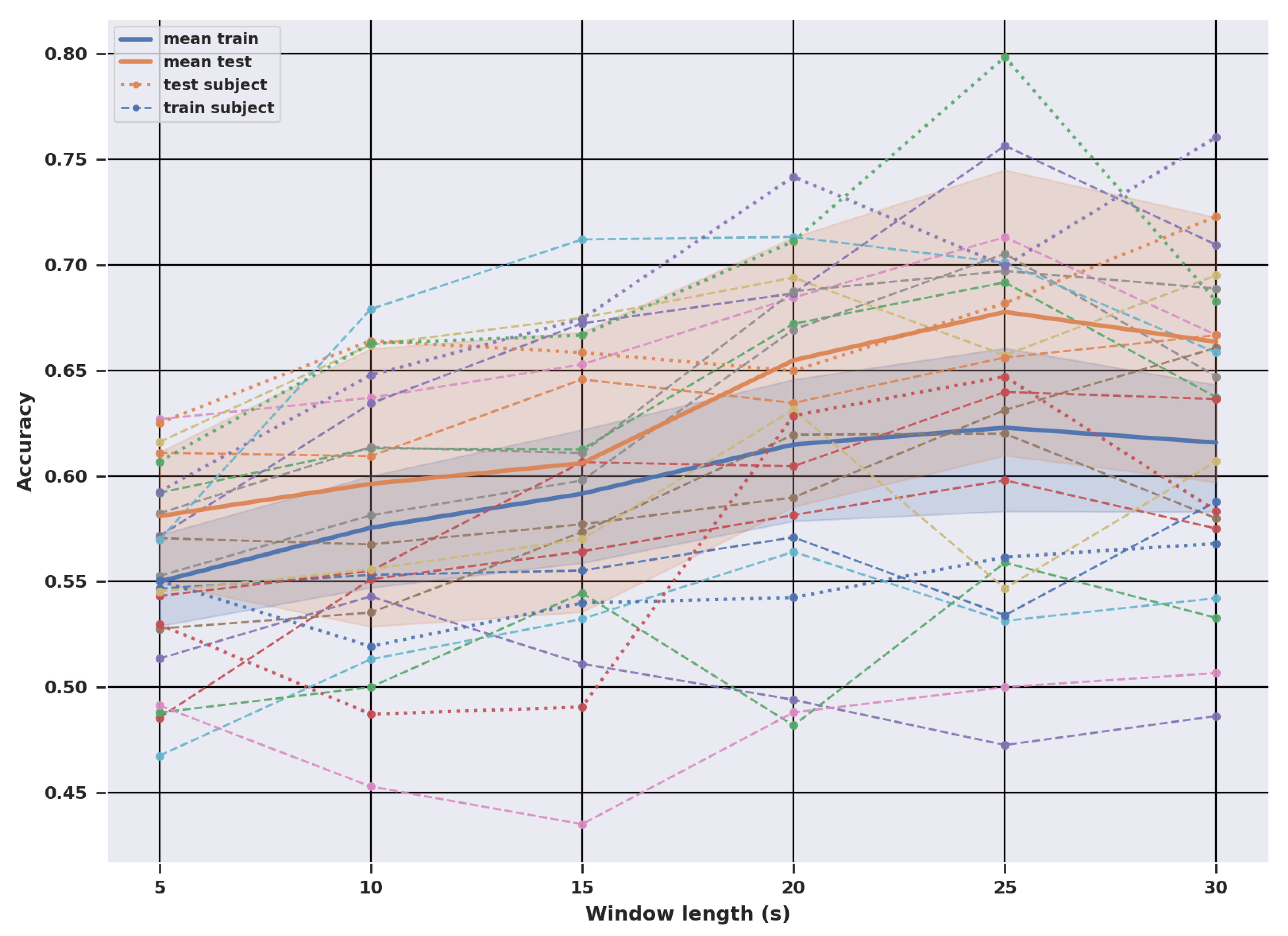
In terms of the overall classification accuracy, shorter windows showed lower performance and the best performance was found for windows of 25 s and 30 s with a statistically insignificant difference between the two. However, even if the differences between other window options were statistically significant, they were modest in absolute terms (lowest accuracy 60% vs. highest accuracy 67.6%). There were also large individual differences and person-specific factors which affected which samples were correctly and incorrectly classified. The individual accuracies ranged from 51% to 80% at a 25 s window length and the individual-specific optimal window length varied between 10 s, 20 s, 25 s, and 30 s.

Although earlier studies that have conducted experiments with different window lengths have not tested for statistical significance and they have mainly used window lengths above 30 s, the overall impression has been similar: longer windows tend to provide better performance. In [32], the best performance was found with a 120 s window and with one exception (15 vs. 30 s) the performance increased as the window length increased. The differences between the window lengths were small in [24], but still, longer windows performed better with nearly all of the tested classifiers.

Compared to the related work mentioned in Table 1, the classification accuracy in this study was rather low at each window length. Still, the highest accuracy (67.6%) at 25 s was almost the same as in the original paper [14] using the same dataset with a 30 s window (68.2%) and higher than in [45] (63.3%) and [46] (62%) using a subset of the same dataset and a 30 s window. The low performance is likely related to large individual differences and the tasks used in the dataset to elicit the cognitive load, which are discussed below.

The six elementary cognitive tasks (ECT) were selected based on [47], where they identified three relevant cognitive capabilities in the ubiquitous computing domain: flexibility of closure (HP), speed of closure (GC) and perceptual speed (FA, NC, PT, SX). However, the ECT refers to any range of basic tasks that require only a small number of mental processes and they have been originally designed to demonstrate individual differences between more than two participant groups (e.g., patients vs. healthy controls) [47]. Therefore, the cognitive load of these six tasks may have been mild compared to the N-back, the working memory task.

Table 8. The proportion of samples correctly classified as cognitive load during each cognitive task, and the number of windows for each task at a window length of 25 s.

	FA	GC	HP	NC	PT	SX	n2	n3
Proportion	0.723	0.469	0.845	0.750	0.638	0.747	0.839	0.730
Windows	382	207	336	388	210	245	168	174

shows the task-wise accuracy for each of the tasks and despite the fact that there were less samples from N-back tasks than the other tasks, they were relatively well-recognized as a cognitive load.

In relation to real-life applications, however, eliciting a relatively mild cognitive load offers a more realistic situation. In real-life, extreme reactions (deep relaxation or high cognitive load) tend to occur rarely and reactions are milder than in laboratory protocols designed to elicit a high cognitive load or stress. All in all, the varying task difficulty between the seven different tasks, the three different task difficulty levels (low, moderate, high) used in the study, as well as the individual differences in cognitive performance and physiological reactions may have affected the varying classification results.

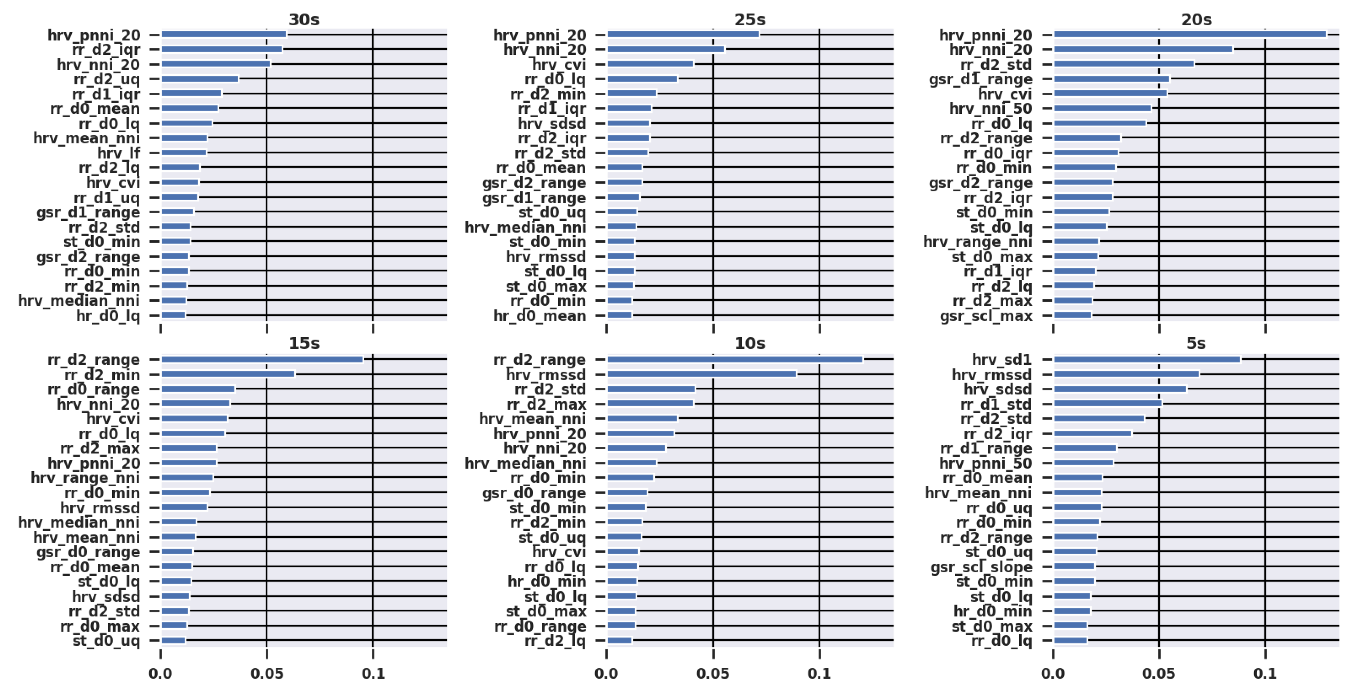
Radüntz et al. [48] suggested that biomarkers, especially heart rate features, exhibit themselves on different timescales in cognitively demanding tasks. They found that the heart rate responded earlier to workload changes than frequency domain HRV parameters. This is in line with the findings in this paper that the most important variables for detecting a cognitive load were statistics of the RR intervals and HRV features from the time- and non-linear domain. Frequency domain variables were among top-20 only at a window length of 30 s, which may indicate that frequency domain measures respond slower than HR-related features from other domains. A similar notion was given in [22], who report that ultra-short frequency domain norms are from 20 to 180 s, and generally windows of 60 s and up to 24 h should be used.

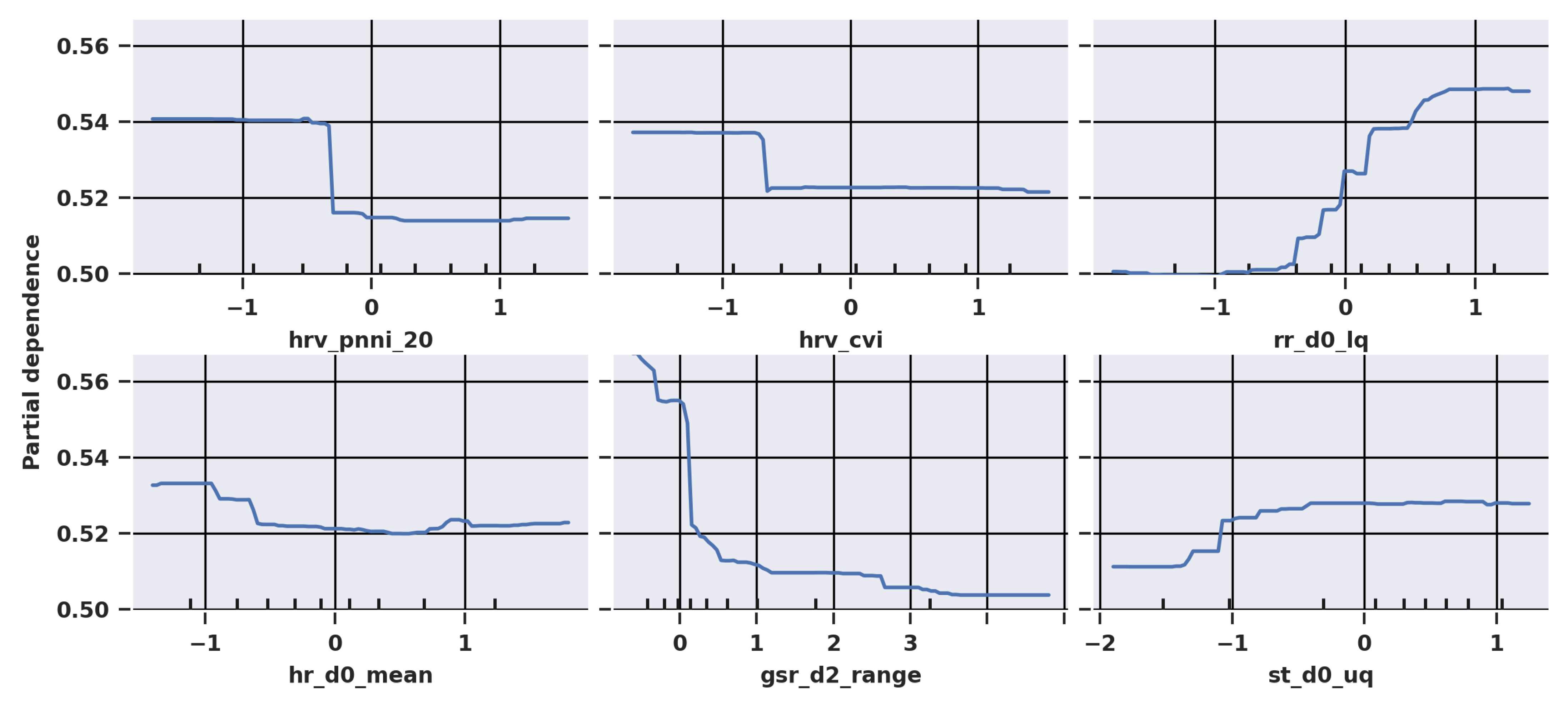
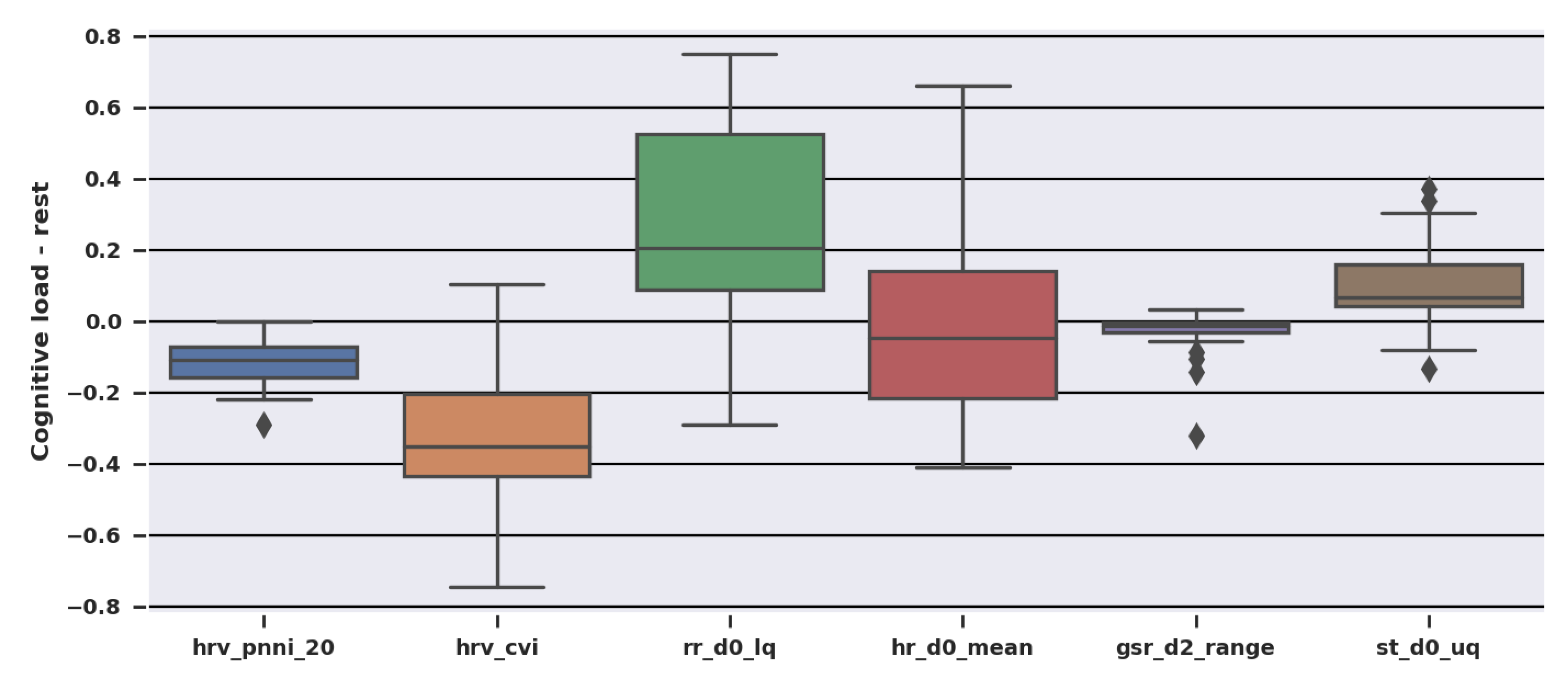
Thus, the tasks were short enough that not all features could respond before the state changed again, which may have affected the feature importances and the direction where the features changed during the tasks. As evidenced in Figure 7, the direction of change between features and individuals varied, and e.g., the HRV was lower in the resting state than in the cognitive load state for some participants. Again, this may be a symptom of the tasks producing a mild cognitive load, but also in the way the resting and cognitive load states were defined. In this study, the states were defined as in the original paper, and the resting state was a combination of all resting periods before and between the cognitive tasks. However, the rest sessions located between the tasks are not similar to the resting state measured as a baseline before the tasks, or at the very end of the measurement protocol. Because people do not recover instantaneously, physiological reactions caused by cognitive tasks are still ongoing when the rest session begins, which likely affected the classification performance. A significantly higher classification performance was found, e.g., in [20], where the resting condition represented a baseline measurement conducted at the beginning and the end of the measurement protocol. However, these kinds of baseline rest periods have not been recorded in this dataset.

An analysis of confusion matrices revealed that errors made by classifying cognitive load periods as resting was quite stable for all the window lengths (between a minimum of 26.2% at 5 s and a maximum of 28.9% at 15 s) whereas the number of errors made by classifying resting as a cognitive load increased as the window length decreased (38.3% at 25 s and increasing to 53.8% at 5 s). Therefore, it seems that the classifier made the most errors when the person was recovering from a cognitive load and that the effect of the used division for cognitive load and resting state may have been especially strong for the shorter window lengths. Analyzing the dynamics of state detection in short windows might reveal more reasons why shorter windows had inferior performance, however, it is beyond scope of this text and is left for future work.

In this study, overlapping was used to utilize the available data more efficiently. Since each task lasted for as long as it took for the subject to complete it, the task length varied between tasks and individuals: easier tasks were completed faster and some subjects were quicker than others. All in all, approximately 34% of the tasks were completed in less than 60 s (needed to have two windows at a 30 s window length without an overlap), 16% in less than 45 s (needed to have two windows at 30 s window length with a 50% overlap), and 23% were completed in less than 50 s (needed to have two windows at a 25 s window length without an overlap) and 10% in less than 37.5 s (needed to have two windows at a 25 s window length with a 50% overlap). So, especially for the longer window lengths, overlapping increased the amount of available data and prevented disregarding data either from the beginning or the end of each task. Although overlapping is often employed in feature extraction (see Table 1) and a 50% overlap is commonly used in signal processing for spectral density estimation [49], its effect on the classification performance in cognitive state detection [9] and human activity recognition [50] has been found to be insignificant. However, overlapping can update the output incrementally and more efficiently than fixed windows [9] and thus it has potential value for future real-time systems with continuous state estimation.

The focus in this study was on cognitive load detection, which is methodologically closely related to affect, or emotion, recognition, where rather long windows are also often employed. Since an affective state tends to last for a very short time [21], shorter feature windows also for affect recognition should be investigated in future studies.

5. Conclusions and Future Work

Cognitive load assessment could serve multiple applications, e.g., in human–computer interaction to recognize and adapt to human overload issues. The future direction in assessing cognitive load is in real-time analysis and detecting the state in a streaming mode. In this study, a step towards more timely, real-time cognitive load detection was taken by analyzing the effect that ultra-short window lengths (30 s or less) have on detection performance.

The results on this dataset showed that longer windows perform better with statistically significant differences. The best performance of 67.6% was observed at a 25 s window length and the accuracy decreased to 60.0% at a 5 s window length. The optimal window length varied on an individual level, and whereas longer windows performed better on average, shorter windows were better for some individuals. Compared to earlier works using longer windows, the classification accuracies obtained were low, but the accuracy on the longer windows tested was similar or higher to those obtained earlier with the same dataset in [14,45,46] using a 30 s window.

The tasks used in the dataset produced rather mild cognitive load, which is closer to real-life circumstances but more difficult to detect than a higher load. Moreover, shorter windows contain less data, and some physiological features could not react on time to changes in the cognitive load and thus were not useful for state detection. R-to-R interval statistics as well as time- and non-linear domain HRV features had the fastest response to changes in cognitive load, followed by GSR statistics and skin temperature.

Short windows allow predicting the state more often, and so they may be more desirable in applications where more timely state detection is needed. However, shorter windows contain less data and physiological events, and so it is more difficult to correctly detect the state with shorter windows than it is with longer windows. Thus, the timeliness will be achieved on the expense of model accuracy as the results of this study demonstrate. The performance on a 5 s window was 7.6% behind of the performance on a 25 s window, despite that it contained five times less data. Although the performance found on this dataset was rather limited, this motivates future studies for real-time, even streaming, cognitive load detection.

Future studies towards this goal would benefit from a larger database to account for individual differences more effectively, to analyze the effects of window overlapping in terms of classification performance and continuous state detection, and to be able to use a larger set of different window lengths. Additionally, the analysis of the effect of short windows could be extended to other state detection tasks within affect recognition, to address similar issues in a broader context.

References

1. Krause, A.J.; Simon, E.B.; Mander, B.A.; Greer, S.M.; Saletin, J.M.; Goldstein-Piekarski, A.N.; Walker, M.P. The sleep-deprived human brain. Nat. Rev. Neurosci. 2017, 18, 404–418. [Google Scholar] [CrossRef] [PubMed]
2. Petruo, V.A.; Mückschel, M.; Beste, C. On the role of the prefrontal cortex in fatigue effects on cognitive flexibility—A system neurophysiological approach. Sci. Rep. 2018, 8, 1–13. [Google Scholar] [CrossRef]
3. Shields, G.S.; Sazma, M.A.; Yonelinas, A.P. The effects of acute stress on core executive functions: A meta-analysis and comparison with cortisol. Neurosci. Biobehav. Rev. 2016, 68, 651–668. [Google Scholar] [CrossRef] [Green Version]
4. Arnsten, A.F.T. Stress signalling pathways that impair prefrontal cortex structure and function. Nat. Rev. Neurosci. 2009, 10, 410–422. [Google Scholar] [CrossRef]
5. Sörqvist, P.; Dahlström, Ö.; Karlsson, T.; Rönnberg, J. Concentration: The neural underpinnings of how cognitive load shields against distraction. Front. Hum. Neurosci. 2016, 10, 1–10. [Google Scholar] [CrossRef] [PubMed] [Green Version]
6. Young, M.S.; Brookhuis, K.A.; Wickens, C.D.; Hancock, P.A. State of science: Mental workload in ergonomics. Ergonomics 2015, 58, 1–17. [Google Scholar] [CrossRef]
7. Won, E.; Kim, Y.K. Stress, the Autonomic Nervous System, and the Immune-kynurenine Pathway in the Etiology of Depression. Curr. Neuropharmacol. 2016, 14, 665–673. [Google Scholar] [CrossRef] [PubMed] [Green Version]
8. Kreibig, S.D. Autonomic nervous system activity in emotion: A review. Biol. Psychol. 2010, 84, 394–421. [Google Scholar] [CrossRef] [PubMed]
9. Anusha, A.S.; Jose, J.; Preejith, S.P.; Jayaraj, J.; Mohanasankar, S. Physiological signal based work stress detection using unobtrusive sensors. Biomed. Phys. Eng. Express 2018, 4. [Google Scholar] [CrossRef]
10. Vinkers, C.H.; Penning, R.; Hellhammer, J.; Verster, J.C.; Klaessens, J.H.G.M.; Olivier, B.; Kalkman, C.J. The effect of stress on core and peripheral body temperature in humans. Stress 2013, 16, 520–530. [Google Scholar] [CrossRef]
11. Larmuseau, C.; Cornelis, J.; Lancieri, L.; Desmet, P.; Depaepe, F. Multimodal learning analytics to investigate cognitive load during online problem solving. Br. J. Educ. Technol. 2020, 51, 1548–1562. [Google Scholar] [CrossRef]
12. Kistler, A.; Mariauzouls, C.; von Berlepsch, K. Fingertip temperature as an indicator for sympathetic responses. Int. J. Psychophysiol. 1998, 29, 35–41. [Google Scholar] [CrossRef]
13. Smets, E.; De Raedt, W.; Van Hoof, C. Into the Wild: The Challenges of Physiological Stress Detection in Laboratory and Ambulatory Settings. IEEE J. Biomed. Health Inform. 2019, 23, 463–473. [Google Scholar] [CrossRef] [PubMed]
14. Gjoreski, M.; Kolenik, T.; Knez, T.; Luštrek, M.; Gams, M.; Gjoreski, H.; Pejović, V. Datasets for cognitive load inference using wearable sensors and psychological traits. Appl. Sci. 2020, 10, 3843. [Google Scholar] [CrossRef]
15. Hidalgo-Muñoz, A.R.; Béquet, A.J.; Astier-Juvenon, M.; Pépin, G.; Fort, A.; Jallais, C.; Tattegrain, H.; Gabaude, C. Respiration and Heart Rate Modulation Due to Competing Cognitive Tasks While Driving. Front. Hum. Neurosci. 2019, 12, 1–8. [Google Scholar] [CrossRef]
16. Visnovcova, Z.; Mestanik, M.; Gala, M.; Mestanikova, A.; Tonhajzerova, I. The complexity of electrodermal activity is altered in mental cognitive stressors. Comput. Biol. Med. 2016, 79, 123–129. [Google Scholar] [CrossRef] [PubMed]
17. Castaldo, R.; Melillo, P.; Bracale, U.; Caserta, M.; Triassi, M.; Pecchia, L. Acute mental stress assessment via short term HRV analysis in healthy adults: A systematic review with meta-analysis. Biomed. Signal Process. Control 2015, 18, 370–377. [Google Scholar] [CrossRef] [Green Version]
18. Dehais, F.; Causse, M.; Vachon, F.; Tremblay, S. Cognitive conflict in human–automation interactions: A psychophysiological study. Appl. Ergon. 2012, 43, 588–595. [Google Scholar] [CrossRef] [Green Version]
19. Paprocki, R.; Lenskiy, A. What does eye-blink rate variability dynamics tell us about cognitive performance? Front. Hum. Neurosci. 2017, 11. [Google Scholar] [CrossRef]
20. Pettersson, K.; Tervonen, J.; Närväinen, J.; Henttonen, P.; Määttänen, I.; Mäntyjärvi, J. Selecting Feature Sets and Comparing Classification Methods for Cognitive State Estimation. In Proceedings of the 2020 IEEE 20th International Conference on Bioinformatics and Bioengineering (BIBE), Cincinnati, OH, USA, 26–28 October 2020; pp. 683–690. [Google Scholar] [CrossRef]
21. Schmidt, P.; Reiss, A.; Dürichen, R.; Laerhoven, K.V. Wearable-based affect recognition—A review. Sensors 2019, 19, 4079. [Google Scholar] [CrossRef] [PubMed] [Green Version]
22. Shaffer, F.; Ginsberg, J.P. An Overview of Heart Rate Variability Metrics and Norms. Front. Public Health 2017, 5, 258. [Google Scholar] [CrossRef] [Green Version]
23. Marshall, S.P. Identifying cognitive state from eye metrics. Aviat. Space Environ. Med. 2007, 78, B165–B175. [Google Scholar]
24. Gjoreski, M.; Luštrek, M.; Gams, M.; Gjoreski, H. Monitoring stress with a wrist device using context. J. Biomed. Inform. 2017, 73, 159–170. [Google Scholar] [CrossRef]
25. Smets, E.; Casale, P.; Großekathöfer, U.; Lamichhane, B.; De Raedt, W.; Bogaerts, K.; Van Diest, I.; Van Hoof, C. Comparison of machine learning techniques for psychophysiological stress detection. In Pervasive Computing Paradigms for Mental Health. MindCare 2015, Communications in Computer and Information Science; Springer: Cham, Switzerland, 2015; Volume 604, pp. 13–22. [Google Scholar] [CrossRef]
26. Castaldo, R.; Montesinos, L.; Melillo, P.; James, C.; Pecchia, L. Ultra-short term HRV features as surrogates of short term HRV: A case study on mental stress detection in real life. BMC Med. Inform. Decis. Mak. 2019, 19, 1–13. [Google Scholar] [CrossRef] [PubMed] [Green Version]
27. Huysmans, D.; Smets, E.; De Raedt, W.; Van Hoof, C.; Bogaerts, K.; Van Diest, I.; Helic, D. Unsupervised learning for mental stress detection exploration of self-organizing maps. In Proceedings of the BIOSIGNALS 2018—11th International Conference on Bio-Inspired Systems and Signal Processing, Part of 11th International Joint Conference on Biomedical Engineering Systems and Technologies (BIOSTEC 2018), Madeira, Portugal, 19–21 January 2018; pp. 26–35. [Google Scholar] [CrossRef]
28. Healey, J.; Nachman, L.; Subramanian, S.; Shahabdeen, J.; Morris, M. Out of the Lab and into the Fray: Towards Modeling Emotion in Everyday Life. In Pervasive Computing; Floréen, P., Krüger, A., Spasojevic, M., Eds.; Springer: Berlin/Heidelberg, Germany, 2010; pp. 156–173. [Google Scholar]
29. Marín-Morales, J.; Higuera-Trujillo, J.L.; Greco, A.; Guixeres, J.; Llinares, C.; Scilingo, E.P.; Alcañiz, M.; Valenza, G. Affective computing ual reality: Emotion recognition from brain and heartbeat dynamics using wearable sensors. Sci. Rep. 2018, 8, 1–15. [Google Scholar] [CrossRef] [PubMed]
30. Guo, H.W.; Huang, Y.S.; Lin, C.H.; Chien, J.C.; Haraikawa, K.; Shieh, J.S. Heart Rate Variability Signal Features for Emotion Recognition by Using Principal Component Analysis and Support Vectors Machine. In Proceedings of the 2016 IEEE 16th International Conference on Bioinformatics and Bioengineering (BIBE 2016), Taichung, Taiwan, 31 October–2 November 2016; pp. 274–277. [Google Scholar] [CrossRef]
31. Stikic, M.; Johnson, R.R.; Tan, V.; Berka, C. EEG-based classification of positive and negative affective states. Brain-Comput. Interfaces 2014, 1, 99–112. [Google Scholar] [CrossRef]
32. Siirtola, P. Continuous stress detection using the sensors of commercial smartwatch. In Proceedings of the UbiComp/ISWC 2019—Adjunct Proceedings of the 2019 ACM International Joint Conference on Pervasive and Ubiquitous Computing and Proceedings of the 2019 ACM International Symposium on Wearable Computers; ACM: London, UK, 2019; pp. 1198–1201. [Google Scholar] [CrossRef] [Green Version]
33. Schmidt, P.; Reiss, A.; Duerichen, R.; Marberger, C.; Van Laerhoven, K. Introducing WESAD, a multimodal dataset for wearable stress and affect detection. In Proceedings of the 2018 on International Conference on Multimodal Interaction (ICMI ’18), Boulder, CO, USA, 16–20 October 2018; ACM Press: New York, NY, USA, 2018; pp. 400–408. [Google Scholar] [CrossRef]
34. Kroupi, E.; Vesin, J.M.; Ebrahimi, T. Subject-Independent Odor Pleasantness Classification Using Brain and Peripheral Signals. IEEE Trans. Affect. Comput. 2016, 7, 422–434. [Google Scholar] [CrossRef]
35. Bota, P.J.; Wang, C.; Fred, A.L.N.; Placido Da Silva, H. A Review, Current Challenges, and Future Possibilities on Emotion Recognition Using Machine Learning and Physiological Signals. IEEE Access 2019, 7, 140990–141020. [Google Scholar] [CrossRef]
36. Jeppesen, J.; Beniczky, S.; Johansen, P.; Sidenius, P.; Fuglsang-Frederiksen, A. Using Lorenz plot and Cardiac Sympathetic Index of heart rate variability for detecting seizures for patients with epilepsy. In Proceedings of the 2014 36th Annual International Conference of the IEEE Engineering in Medicine and Biology Society (EMBC 2014), Chicago, IL, USA, 26–30 August 2014; pp. 4563–4566. [Google Scholar] [CrossRef]
37. Tervonen, J.; Puttonen, S.; Sillanpää, M.J.; Hopsu, L.; Homorodi, Z.; Keränen, J.; Pajukanta, J.; Tolonen, A.; Lämsä, A.; Mäntyjärvi, J. Personalized mental stress detection with self-organizing map: From laboratory to the field. Comput. Biol. Med. 2020, 124, 103935. [Google Scholar] [CrossRef]
38. Chen, T.; Guestrin, C. XGBoost: A scalable tree boosting system. In Proceedings of the 22nd ACM SIGKDD International Conference on Knowledge Discovery and Data Mining, San Francisco, CA, USA, 13–17 August 2016; ACM: New York, NY, USA, 2016; Volume 19, pp. 785–794. [Google Scholar] [CrossRef] [Green Version]
39. Fernández-Delgado, M.; Cernadas, E.; Barro, S.; Amorim, D. Do we need hundreds of classifiers to solve real world classification problems? J. Mach. Learn. Res. 2014, 15, 3133–3181. [Google Scholar] [CrossRef]
40. Frazier, P.I. A Tutorial on Bayesian Optimization. arXiv 2018, arXiv:1807.02811. [Google Scholar]
41. Pedregosa, F.; Varoquaux, G.; Gramfort, A.; Michel, V.; Thirion, B.; Grisel, O.; Blondel, M.; Prettenhofer, P.; Weiss, R.; Dubourg, V. Scikit-learn: Machine Learning in Python. J. Mach. Learn. Res. 2011, 12, 2825–2830. [Google Scholar]
42. Champseix, R. Heart Rate Variability Analysis. 2018. Available online: https://github.com/Aura-healthcare/hrvanalysis (accessed on 18 January 2021).
43. Makowski, D.; Pham, T.; Lau, Z.J.; Brammer, J.C.; Lespinasse, F.; Pham, H.; Schölzel, C.; Chen, S.H.A. NeuroKit2: A Python Toolbox for Neurophysiological Signal Processing. Behav. Res. Methods 2020. [Google Scholar] [CrossRef]
44. Bergstra, J.; Yamins, D.L.K.; Cox, D.D. Making a Science of Model Search: Hyperparameter Optimization in Hundreds of Dimensions for Vision Architectures. In Proceedings of the 30th International Conference on Machine Learning (ICML’13), Atlanta, GA, USA, 16–21 June 2013; Volume 28, pp. 115–123. [Google Scholar]
45. Li, X.; De Cock, M. Cognitive load detection from wrist-band sensors. In UbiComp/ISWC 2020 Adjunct—Proceedings of the 2020 ACM International Joint Conference on Pervasive and Ubiquitous Computing and Proceedings of the 2020 ACM International Symposium on Wearable Computers; ACM: Cancun, Mexico, 2020; pp. 456–461. [Google Scholar] [CrossRef]
46. Salfinger, A. Deep learning for cognitive load monitoring: A comparative evaluation. In UbiComp/ISWC 2020 Adjunct—Proceedings of the 2020 ACM International Joint Conference on Pervasive and Ubiquitous Computing and Proceedings of the 2020 ACM International Symposium on Wearable Computers; ACM: Cancun, Mexico, 2020; pp. 462–467. [Google Scholar] [CrossRef]
47. Haapalainen, E.; Kim, S.; Forlizzi, J.F.; Dey, A.K. Psycho-physiological measures for assessing cognitive load. In UbiComp’10—Proceedings of the 2010 ACM Conference on Ubiquitous Computing; ACM: Copenhagen, Denmark, 2010; pp. 301–310. [Google Scholar] [CrossRef]
48. Radüntz, T.; Mühlhausen, T.; Freyer, M.; Fürstenau, N.; Meffert, B. Cardiovascular Biomarkers’ Inherent Timescales in Mental Workload Assessment During Simulated Air Traffic Control Tasks. Appl. Psychophysiol. Biofeedback 2020. [Google Scholar] [CrossRef] [PubMed]
49. Heinzel, G.; Rüdiger, A.; Schilling, R. Spectrum and Spectral Density Estimation by the DISCRETE Fourier Transform (DFT), Including a Comprehensive List of Window Functions and Some New at-Top Windows. (unpublished). 2002, 1–84. Available online: https://holometer.fnal.gov/GH_FFT.pdf (accessed on 18 January 2021).
50. Dehghani, A.; Sarbishei, O.; Glatard, T.; Shihab, E. A Quantitative Comparison of Overlapping and Non-Overlapping Sliding Windows for Human Activity Recognition Using Inertial Sensors. Sensors 2019, 19, 5026. [Google Scholar] [CrossRef] [Green Version]
Figure 1. Pipeline followed in data processing and evaluating the results.
Electronics 10 00613 g001
Figure 2. Progress of the Bayesian parameter optimization, (i) test accuracy obtained at each iteration with leave-two-out validation (top panel), and (ii) the cumulative maximum accuracy obtained by each iteration (bottom panel).
Electronics 10 00613 g002
Figure 3. Posteriors of the max_depth parameter, describing the depth of each tree in the ensemble, after 300 Bayesian optimization iterations at each window length. Vertical lines denote the best value found.
Electronics 10 00613 g003
Figure 4. Importance of the top-20 features for each window length.
Electronics 10 00613 g004
Figure 5. Partial dependency plots of selected features for the model with 25 s window length.
Electronics 10 00613 g005
Figure 6. Classification accuracy observed with the dataset’s default train-test split using the XGB model with default hyperparameters (ablating Bayesian optimization). Solid lines denote mean accuracy with confidence regions obtained by bootstrapping around them. Dashed lines depict the validation (training-split) and dotted lines the test (test-split) accuracy of a single subject.
Electronics 10 00613 g006
Figure 7. Difference of selected mean feature values between cognitive load and rest sessions across each individual, computed with 25 s window length. Positive values denote that the feature value was higher in cognitive load. Differences of rr_d0_lq and hrv_pnni_20 were scaled by dividing by 100, and hr_d0_mean by dividing by 10 to show the distribution of each feature better.
Electronics 10 00613 g007