A Comparison of Deep Learning Methods for Timbre Analysis in Polyphonic Automatic Music Transcription

Abstract

Automatic music transcription (AMT) is a critical problem in the field of music information retrieval (MIR). When AMT is faced with deep neural networks, the variety of timbres of different instruments can be an issue that has not been studied in depth yet. The goal of this work is to address AMT transcription by analyzing how timbre affect monophonic transcription in a first approach based on the CREPE neural network and then to improve the results by performing polyphonic music transcription with different timbres with a second approach based on the Deep Salience model that performs polyphonic transcription based on the Constant-Q Transform. The results of the first method show that the timbre and envelope of the onsets have a high impact on the AMT results and the second method shows that the developed model is less dependent on the strength of the onsets than other state-of-the-art models that deal with AMT on piano sounds such as Google Magenta Onset and Frames (OaF). Our polyphonic transcription model for non-piano instruments outperforms the state-of-the-art model, such as for bass instruments, which has an F-score of 0.9516 versus 0.7102. In our latest experiment we also show how adding an onset detector to our model can outperform the results given in this work.

1. Introduction

Automatic Music Transcription (AMT) is the capability of transcribing music audio into music notation and it is one of the main research tasks in the fields of music signal processing and music information retrieval (MIR), and one of the most competitive tasks in music information retrieval evaluation eXchange (https://www.music-ir.org/mirex/wiki/MIREX_HOME, accessed on March 2021) [1,2]. Although transcribing a monophonic recording is considered to be a solved problem, AMT still remains an open research problem when it comes to mixed signals with multiple instruments and polyphonic music [3].

AMT approaches can be organized into four subtasks or categories: multi-pitch estimation (MPE) or frame-level transcription, note-level transcription also known as note tracking (NT), stream-level transcription and notation-level transcription. These categories stand for the level of abstraction of the music notation that it is desirable to achieve.

Previous studies addressed AMT by two principal methods: Non-Negative Matrix Factorization (NMF) and Neural Networks (NNs). NN methods usually use spectrograms as inputs to later process the spectrograms with different neural network structures: long short-term memory layers or CNNs, for example. A high number of AMT works use NN and they are based on polyphonic piano transcription. An example of these models is Google Magenta Onsets and Frames (OaF) [4] which is composed by two heads, the onsets head and the frames head. A description of these piano transcription approaches is presented in Section 1.2. There are new approaches that present alternative methods that improve the transcription accuracy by reconstructing the input spectrogram [5]. However, these approaches are trained and tested with piano tracks, but there is a lack of information about the behavior of these models using other instrument families or comparing them with different onset envelopes.

Other studies address AMT by taking a mixed-signal and apply multi-task deep learning, so they perform AMT after separating the sources of the signal which implies the addition of a source separation head to the network. Cerberus [6] uses three heads which correspond to a sources separation head, a deep clustering head and a transcription head and combines them in multi-task deep learning to address AMT problem. New studies on AMT address the multi-instrument music transcription, which also requires to perform the instrument identification subtask, with a self-attention mechanism [7].

As it is described above, AMT can be divided in subcategories. Our AMT approaches are based on attempting AMT by doing frame-level and then note-level transcription, but not both at the same time as previous works that have been introduced above. A brief introduction of the AMT subsections are described below.

1.1. Frame-Level Transcription

The first step in single-instrument AMT is the frequency estimation. There are two subcategories in this level: Fundamental Frequency Estimation (f0 estimation) and Multi-f0 estimation.

Fundamental frequency estimation. Fundamental frequency estimation has been studied over decades. The estimation of f0 consists of the identification of the fundamental frequency of the notes that are present in each time frame (of the order of 10 ms). Some approaches to estimate f0 in monophonic signals are based on template matching with the spectrum of a waveform such as SWIPE [8], and a probabilistic variant of the YIN algorithm [9] that uses a Hidden Markov Model (HMM) to decode the most probable sequence of pitch values, pYIN [10]. Other methods try to estimate the predominant f0 in polyphonic signals by using the so-called salience function [11]. The most recent and best-performing methods such as CREPE [12], use deep learning approaches to address the f0 estimation by converting the input signal into spectrograms and pass them through CNNs.

Multi-f0 estimation. Multi-f0 estimation is the estimation of the multiple fundamental frequencies that are present in a polyphonic signal. In this case, multiple notes are simultaneously present in each time frame. Previous studies of multi-f0 estimation model spectral peaks [13] or learn salience representations for estimating fundamental frequencies by using CNNs with the constant Q-Transform as their inputs [14].

1.2. Frame-Level and Note-Level Transcription in Polyphonic Music

As we introduced in Section 1.1, the piano is the most studied instrument when it comes to polyphonic music transcription. The handful of datasets for piano transcription and the fact that the piano is an instrument with an onset similar to percussive instrument onsets makes the piano the main case of study when it comes to multi-f0 estimation. These models are almost end-to-end models based on CNNs and LSTMs [15,16]. The term end-to-end means that an input is taken and AMT is performed with just deep NNs. In AMT, as it is done in other MIR tasks, some models need to apply subtasks separately. Some models use the signal in the waveform domain as the input of a deep NN and other need a preprocessing step to convert the waveform to a time-frequency representation of the signal, so they can be called end-to-end models.

Onset and Frames (OaF) [4] is a model developed to address polyphonic piano and drums transcription by detecting note onsets and pitch prediction. Depending on the dataset used to train the model it can be used to transcribe piano with the MAESTRO dataset [17] or drums with the Expanded MIDI Groove (E-GMD) dataset [18]. Other models such as [5] also try to transcribe piano. These models are trained with input spectrograms which [19] demonstrate to be the best input for the AMT task. These models have demonstrated to perform well on piano datasets because their architecture reinforces the transcription quality by predicting the onsets which can be well estimated for piano pieces, but there is no evidence on how these models perform with instruments that have different timbres and onset envelopes.

1.3. Stream-Level Transcription

Stream-level transcription is also known as Multi-Pitch Streaming (MPS), timbre tracking or instrument tracking. It takes the note-level transcription where notes are grouped in events and targets them into streams, being each stream one instrument or voice. This is related to source separation tasks where a mixed signal is taken and then separated into multiple instruments and then AMT is performed [6,7,20]. The inputs of these models are mixtures where multiple instruments are present. The frame-level transcription in this case is called multi-pitch streaming and the note-tracking of the single instrument transcription is defined as note streaming. There are also different approaches in this task that correspond to the instrument information. This refers to whether the model is capable of identify the instruments (agnostic) or if it needs information about the genre to dismiss some channels that correspond to instruments that are not probable to be in the mixture (informed). These methods do not perform as well as frame-level or note-level methods of single-instrument transcription due to the fact that the input is not an isolated instrument but a mixture, and this introduces an additional loss that worsens the final transcription. In our work, we do not focus on this AMT level because we perform single-instrument AMT.

1.4. Notation-Level

Notation-level transcription aims to transcribe music from an audio file into a human-readable musical score. This type of transcription requires a deeper understanding of musical structures, including harmonic (key and chords), rhythmic (beats and bars that allows us to quantize the notes) and stream structures. Previous works on notation-level transcription are related to timing quantization [21] among others, and there are some approaches that use deep learning [22] for this purpose. Some of these models [22] try to face this problem with end-to-end models which take a signal or time-frequency representation as their input and they output the score of the musical piece. Other methods [21] do not try to implement an end-to-end approach but they focus on the transcription from a MIDI file to a score. This AMT level deviates from our work due to the fact that our methods try to improve the frame-level and note-level AMT subtasks.

In our work, we describe two methods: in the first method we perform f0 detection and in the second method we detect multi-f0 followed by the corresponding note tracking algorithms. We perform f0 estimation with the CREPE pre-trained weights and then we use the model output to perform the note tracking. We test our results over multiple music instruments with different timbres and we compare the results with the state of the art OaF model that we have also tested with the same instruments despite it being designed for polyphonic piano transcription, so we can see how timbre affects the pitch estimation and note tracking. After the first timbre analysis a multi-f0 model has been trained that allows us to transcribe polyphonic signals of single instruments in a wide range of timbres.

This paper is structured as follows: in this Section 1 we introduce AMT and the previous studies on frame-level and note-level transcription, in the Section 2 we describe the two methods proposed in our work, in the Section 3 we show the results of each of our methods comparing them with the state of the art results, in the Section 4 we discuss the results exposed in Section 3 and finally, in Section 5 we discuss possible next steps and future work.

2. Methods

2.1. Method 1: Monophonic Note-Level Transcription

In this method, we perform monophonic AMT to analyze how timbre affects the AMT results. To do this, we take a clean stem of an instrument as an input, so we have to approach the music transcription task by applying in order some MIR tasks such as f0 estimation and note tracking (Figure 1). The f0 is estimated using the pre-trained CREPE NN and we have implemented and tested a note-tracking algorithm. The innovation presented by this method is the combined use of a deep NN for f0 estimation with a subsequent note tracking algorithm. The tracking algorithm uses the confidence values provided by the last layer of the NN to reinforce the quality of the transcription.

CREPE takes 1024 raw audio samples with a 16 kHz sample rate as its input, passes them through a CNN of 6 layers followed by a fully connected layer at the end, and its output is a 360-dimensional vector that corresponds to a specific pitch value defined in cents. The 360 pitch values are denoted as $c_i$ where $i=1,...,360$ in order to cover six octaves with 20-cent intervals between 32.70 Hz (C1) and 1975.5 Hz (B7). Cent is a distance measure which represents music intervals respect to a reference pitch ($f_{ref}$) in Hz, defined as a function of frequency f in Hz. Cents provide a logarithmic pitch scale, with 100 cents corresponding to a distance of one semitone. Equation (1) shows the relationship between frequency (f) and cents (c):

$$c\left(f\right)={log}_2\frac{f}{f_{ref}}$$

(1)

where $f_{ref}$ = 10 Hz as it is described in [12].

As it is described in [12], CREPE model is trained with a binary cross entropy loss function. The resulting pitch estimate $\widehat{c}$ is a weighted average of pitches $c_i$ according to the output ${\widehat{y}}_i$, which is the estimated frequency in Hz:

$$\widehat{c}=\frac{{\sum }_{i=1}^{360}{\widehat{y}}_i{c}_i}{{\sum }_{i=1}^{360}{\widehat{y}}_i}$$

(2)

$$\widehat{f}=f_{ref}·2^{\widehat{c}/100}$$

(3)

There are 5 different CREPE models depending on the capacity: tiny, small, medium, large and full. We take the full model and we do not apply temporal smoothing to the pitch curve.

Note Tracking (NT) Algorithm

Our note tracking algorithm is based on the minimum confidence value that CREPE NN outputs in each time step. Some studies in different MIR tasks such as audio synthesis fix this value around 85% [23], however, we estimate this value by building the histogram of confidences that the CREPE NN outputs.

The minimum confidence value (c) can be estimated by different approaches based on the histogram of the estimated confidences that the frequencies have for every time step of 10 ms. In our work, we have used a triangulation algorithm, a gaussian distribution over the frequencies histogram and the Otsu’s thresholding algorithm. A histogram of confidences of a Slakh2100 dataset track is shown in Figure 2. We show how we obtain the minimum confidence for each of the proposed methods: triangulation algorithm (Figure 2a), gaussian (Figure 2b) and Otsu’s threshold (Figure 2c).

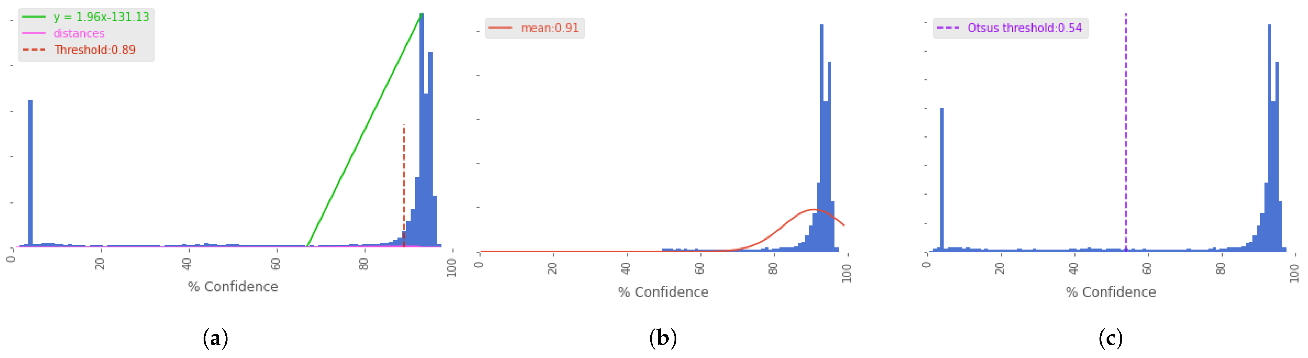
• Triangulation algorithm. To perform the triangulation algorithm we calculate the maximum value of the histogram to its right (close to one) and the nearest minimum value to the maximum at its left. Then, we obtain the line that passes through this maximum and minimum values and we compute the distance from each point of the histogram between the minimum and maximum values to the line. The optimum threshold is equal to the minimum confidence value. This value is the one that maximizes the distance from the histogram points to the line.
• Gaussian distribution. This approach is based on fitting the right part of the histogram (confidences from 0.5 to 1) built from the CREPE output with a gaussian distribution and taking the mean as the minimum confidence value.
• Otsu’s threshold [24]. This method is most often used by the image processing community to perform image thresholding. In these applications the algorithm returns a threshold which separates two classes of pixels by computing the histogram built with the pixel distributions. Here, we use this method to predict the minimum confidence value by taking the minimum confidence histogram of CREPE’s output.

The tracking algorithm designed for this work takes the output of the CREPE NN and groups constant frequencies over time depending on their confidence. The algorithm takes as its inputs the outputs of the CREPE network that are a list or arrays of frequency, time and confidence and outputs a MIDI file by writing the Note ON, Note OFF and pitch events. There is an additional input passed to the algorithm that we call minimum confidence which is the minimum pitch confidence that our algorithm uses to group the same pitch values over time. Pitch confidences below the minimum confidence value are discarded. Once we have all the note events we discard the notes within which the duration is smaller than 50 ms. We set the output of CREPE NN to a time step of 10 ms, so the model predicts an estimated frequency and confidence every 10 ms along the duration of the audio file. The developed algorithm is shown in Algorithm 1.

Algorithm 1: Tracking algorithm.

2.2. Method 2: Polyphonic Note-Level Transcription

Due to the fact that many instruments are polyphonic we introduce a second method to improve the monophonic transcription by implementing a multi-f0 transcription. In this case, the neural network will be trained with multiple timbres with which CREPE has not been trained. The main innovation of this method is the study of the behavior of a deep NN for multi-f0 estimation with different instrument families. This NN uses as input the CQT and its harmonics to perform, subsequently, the training of the model. In this way, we can demonstrate the importance of the timbre and the onsets envelope of different instrument families for the correct note identification in AMT. Furthermore, in this method (Figure 3), we propose the addition of an onsets detection stage to the implemented NN that improves the results presented in this work.

This method is based on Deep Salience [14], a neural network that learns a series of convolutional filters that produce a salience representation. This network uses the harmonic constant-Q transform (HCQT) as the input representation of a CNN. The HCQT is defined as a 3-dimensional vector which dimensions are: frequency (f), time (t) and harmonic (h), which corresponds to the h-th harmonic of the frequency f and time t. Harmonics are defined to be greater than zero ($h>0$) so the CQT is computed as a standard CQT with the same frequency resolution of octaves for all harmonics and the minimum frequency is scaled by the harmonic $h\times f_{min}$. The input of the CNN is the time-frequency CQT vector of depth equal to the number of harmonics that we compute.

The harmonics can be obtained as powers of 2, $h=2^n$ being n an integer number. This means that the k-th frequency can be obtained using Equation (4):

$$f_k=h\times f_{min}\times 2^{k/B}$$

(4)

with B equal to the number of bins per octave.

Following [14], we compute 6 harmonics that corresponds to h = 0.5, 1, 2, 3, 4 and 5, being h = 1 to the fundamental and h = 0.5 one subharmonic below the fundamental. We compute the CQTs with a hop size value of 512 samples, B = 60 bins per octave, 6 octaves and $f_{min}$ = 32.7 Hz which corresponds to the C1 note.

In our implementation, we do not calculate the CQTs for the entire tracks at once to pass them to the CNN but we calculate a CQT slice with a margin of 64 × 512 samples to the right and left part of the slice. This process allows us to reduce the training time of the model although the resolution in the low-frequency region is not as good as if we compared to calculating the CQT of the whole audio file at once and divide it in CQT slices. The selected margin of 64 × 512 samples ensures that the resolution loss does not affect the results of the transcription metrics P, R and F-score (see Section 3) due to the fact that there is no strong presence of notes in the low frequencies range. The final CQT dimensions used in our model are 50 time frames and 360 frequency bins. We calculate the CQTs with the librosa library [25], implemented in python. In Figure 4 left, we show an example of a slice of CQT obtained with our method and in the right we show the same slice of the CQT in the left side of the figure but in this case the CQT has been calculated for the entire song. As Figure 4 shows, there is no difference between the CQT slice obtained with our method and the one obtained by calculating the CQT of the entire song.

Adapting the structure proposed in [14], the CNN of our model is shown in Figure 5 and has about 406.000 parameters. It contains 6 convolutional layers. The first 5 convolutional layers are followed by Relu activations and Batch Normalization layers and the 6th layer is followed by a sigmoid activation function that maps each bin’s output to the range [0,1]. We use the Adam optimizer [26] and cross-entropy loss function. The output of the CNN is a 2-dimensional matrix. The time dimension is equal to the input CQT slice dimension and the frequency dimension is equal to 72 that corresponds to the pitch range between C1 and C7 (6 octaves). An important aspect to emphasize is the fact that we do not obtain frequencies in the output of our model, but pitch values that allow us to directly perform the note tracking in a further step.

After training the model, we apply a threshold to discard any predicted pitches which are in a range of [0, 1] due to the sigmoid activation function that is in the last layer of our model, thus we convert these values to just zeros (no note) and ones (note). To calculate this threshold we take 100 random instrument tracks of the Slakh2100 dataset. We take the threshold which gives the maximum F-score obtained in each track, and then we calculate the mean of all the thresholds. In Figure 6 we show how the F-score changes given different threshold values.

The obtained threshold for the database is equal to 0.44 when training the model with all the instrument families of the Slakh2100 dataset. In other experiments of our work, the threshold value will vary when training our model with isolated instrument families. This is because, as explained in Section 3, we train our model with different instrument families so we calculate a threshold for each family.

3. Experiments and Results

3.1. Datasets

For our first method, we take a CREPE pretrained model that has been trained with audio of 16 kHz sampling rate of the following datasets: MIR-1K [27], Bach10 [13], RWC-Synth [10], MedleyDB [28], MDB-STEM-Synth [29], NSynth [30].

We test the f0 detection and note tracking algorithm (Algorithm 1) in the Slakh2100 dataset [31] which provides MIDI files and their synthesized audio files, and we compare the performance of this approach with the OaF model [4]. It is important to note that the tests have been performed on the same dataset although the OaF model has only been trained with the MAESTRO dataset [17] only for piano transcription. Note that we are testing a monophonic transcription model with a dataset of polyphonic instruments and we are comparing the performance with a model (OaF) that has been trained for piano polyphonic transcription. This will lead our results to be non-comparable with OaF model, but our overall goal is to see the impact of the different timbres on AMT, and based on our observations to later train a polyphonic model (see Section 2.2) and improve the transcription results.

For our second method, we train the CNN model for polyphonic transcription with the Slakh2100 dataset [31]. It contains 145 h of mixtures and a total of 2100 automatically mixed tracks and their corresponding MIDI files synthesized. The train, validation and test splits are shown in

Table 1. Train, validation and test splits in Slakh2100 dataset.

Instrument	Train	Validation	Test
Total	12782	3198	1893
Piano	2458	634	380
Bass	1578	374	233
Guitar	3831	991	569
Strings	2381	142	86
Reed	550	600	345
Brass	627	134	92
Chromatic Precussion	317	130	85
Flute	514	67	42
Organ	526	126	61

.

We have tested our model with the split test data from the Slakh2100 dataset, with the Bach10 dataset and the MedleyDB dataset.

3.2. Evaluation Metrics

3.2.1. Method 1: Monophonic Note-Level Transcription

AMT (note-level transcription) is evaluated with Precision (P), Recall (R) and F-measure (F). These metrics can be obtained with the mir_eval python module [32] and they compare the onsets, offsets and pitches of the tracked or predicted notes with the ground truth. An estimated note is considered correct if its onset is within a tolerance of 50ms of the reference note, if its pitch is within a tolerance of 50 cents (which corresponds to a quarter tone) of the reference note, and if its offset is within a tolerance of 50ms of the reference note. Note velocities have not been analyzed in this work. The expressions corresponding to Precision (P), Recall (R), F-score (F${}_1$) and Accuracy (A) are shown in Equations (5)–(7) and (9) respectively [33]. The final F-score is computed with a $\beta =1$ and it is given in Equation (8).

$$\mathrm{Precision}:\mathrm{P}=\frac{\mathrm{TP}}{\mathrm{TP}+\mathrm{FP}}$$

(5)

$$\mathrm{Recall}:\mathrm{R}=\frac{\mathrm{TP}}{\mathrm{TP}+\mathrm{FN}}$$

(6)

$$\mathrm{F}\mathrm{score}:{\mathrm{F}}_{\beta }=(1+{\beta }^2)\times \frac{\mathrm{P}\times \mathrm{R}}{{\beta }^2\times \mathrm{P}+\mathrm{R}}$$

(7)

$$\mathrm{F}\mathrm{score}:{\mathrm{F}}_1=\frac{\mathrm{P}\times \mathrm{R}}{\mathrm{P}+\mathrm{R}}$$

(8)

$$\mathrm{A}=\frac{\mathrm{TP}}{\mathrm{TP}+\mathrm{FP}+\mathrm{FN}}$$

(9)

In the above equations, TP (True Positives) are the estimated events of a given class that start and end at the same temporal positions as reference events of the same class within a time-window of specified tolerance, FP (False Positives) are the estimated events of a given class that start and end at temporal positions where no reference events of the same class do, within a time-window of specified tolerance, and FN (False Negatives) are reference events of a given class that start and end at temporal positions where no estimated events of the same class do for a tolerance time-window.

In Figure 7 we show the transcription (note-level) results for different instrument families in Slakh2100 dataset. Figure 7a shows the comparison between the three minimum confidence prediction methods: triangulation, Gaussian and Otsu. On the other hand, Figure 7b compares the transcription results of the CREPE network with our note tracking algorithm with those obtained with the OaF implementation using the Slakh2100 database.

The results show that, in general, OaF model performs better due to the fact that the prediction of the onset allows the model to transcribe notes in a more efficient way and because of the presence of polyphony in the stems that CREPE cannot predict. Despite this, we can see that the performance of both methods decreases when testing different timbres and instruments whose onsets are not as pronounced as percussive or plucked string instruments. The OaF model suffers more with non-percussive and non-plucked instruments because it does not detect onsets as well as in percussive instruments, and the CREPE NN suffers more with timbral variations which may be because some of our test timbres were not in the dataset with which CREPE was trained. This makes the estimation of f0 with CREPE worse and leads to a decrease in the quality of the music transcription results when performing the note-tracking algorithm.

3.2.2. Method 2: Polyphonic Note-Level Transcription

To improve the results obtained with CREPE plus the note tracking algorithm approach, we train a CNN on polyphonic music (see Section 2.2). To evaluate the results of this method we test our model on the Slakh2100 test split (see Table 1) and we also test the model on the Bach10 and MedleyDB datasets. The metrics that are used to measure the multi-f0 prediction are the following ones: Raw Chroma Accuracy (CA), Accuracy (A), Recall (R), Precision (P) and F-score (F) and Accuracy (A) [33]. Raw Chroma Accuracy measures the pitch accuracy by mapping pitches into one octave so octave errors are ignored. Following the definition given by Bosch et al. in [34] the Raw Croma Accuracy (CA) is defined by the expression shown in Equation (10).

$$\mathrm{CA}=\frac{N}{{\sum }_i{v}_i}$$

(10)

where N is the number of chroma matches and v the ground truth of melodic pitches (voiced).

In

Table 2. Multi-f0 metrics of our model for Slakh2100, Bach10 and MedleyDB datasets. Best result for every metric is highlighted in bold.

Test Dataset	Instrument	CA	Accuracy	R	P	F
Slakh2100	Piano	80.42	78.83	88.39	88.16	87.28
	Bass	85.78	76.08	83.14	84.66	83.36
	Guitar	70.85	67.50	80.07	80.34	78.67
	Strings	82.94	82.01	85.68	91.96	87.96
	Reed	75.88	75.42	82.46	88.24	84.67
	Brass	72.55	50.66	54.72	65.61	58.44
	Chromatic Percussion	21.15	15.05	21.44	30.75	23.82
	Pipe	78.80	77.04	84.95	88.27	86.49
	Organ	68.43	55.32	70.84	65.60	67.00
Bach10	Bach10single	82.37	70.86	84.06	81.00	82.48
	Bach10multi	69.71	67.39	73.93	88.39	80.47
MedleyDB	All	51.89	47.18	68.73	56.89	61.01

we show the multi-f0 metrics results for all the instruments of the Slakh2100 dataset and the means of the metrics obtained testing our model with Bach10 single (separated instruments) and multi (mixed tracks), and MedleyDB datasets calculated with the multipitch functions of the mir_eval library. In Figure 8 we show the results of our model tested in MeldleyDB (Figure 8a), on the Slakh2100 pianos (Figure 8b), and in Bach10 multi (Figure 8c) and Bach10 single (Figure 8d) datasets.

Analyzing the results, we can see the high performance of the piano, bass and strings instruments. The string instruments analyzed in our first method yield poor results due to the fact that this family of instruments presents less percussive onsets than other instruments like the piano, but with our second method we demonstrate that this method is less dependent on the shape of the attack that the notes played on the instrument exhibit.

We show the final transcription comparison results of our model in

Table 3. Transcription metrics of our first model (CREPE + NT) which is monophonic and our second model (CNN) which is polyphonic, and OaF test with Slakh2100 dataset. Best result for every metric is highlighted in bold.

Instrument	Threshold	Note without Offset			Note with Offset
		P	R	F	P	R	F
Piano (CNN)	0.44	65.42	78.72	67.07	30.91	39.06	33.45
Piano (CREPE + NT)	Gaussian	39.01	26.77	30.00	19.39	13.94	15.34
Piano (OaF [4])	-	88.47	94.73	90.68	58.48	63.93	60.49
Bass (CNN)	0.44	68.65	85.96	74.81	53.87	65.02	57.48
Bass (CREPE + NT)	Otsu	48.18	68.06	55.75	44.22	62.32	51.12
Bass (OaF [4])	-	65.98	78.52	71.02	62.39	73.85	66.94
Guitar (CNN)	0.44	55.36	73.25	59.73	36.77	45.85	40.19
Guitar (CREPE + NT)	Otsu	28.19	43.21	31.68	14.08	23.10	16.81
Guitar (OaF [4])	-	55.20	84.95	64.32	39.92	60.63	46.43
Strings (CNN)	0.44	34.24	62.32	41.70	17.91	26.27	20.29
Strings (CREPE + NT)	Otsu	3.54	8.12	4.56	13.06	29.77	16.31
Strings (OaF [4])	-	40.16	81.03	48.88	15.78	30.25	19.72
Reed (CNN)	0.44	66.12	75.84	69.23	51.76	57.68	53.57
Reed (CREPE + NT)	Otsu	24.87	38.16	28.54	9.63	14.70	11.12
Reed (OaF [4])	-	42.91	75.69	52.95	24.99	43.91	30.91
Brass (CNN)	0.44	49.32	58.64	49.98	39.35	41.52	39.25
Brass (CREPE + NT)	-	30.17	40.12	32.15	10.75	14.34	11.79
Brass (OaF [4])	-	45.11	68.53	48.99	37.28	52.42	39.59
Chromatic Perc. (CNN)	0.44	25.77	26.07	22.97	4.99	3.98	4.04
Chromatic Perc. (CREPE + NT)	Triang.	26.40	26.28	23.44	13.24	13.30	11.82
Chromatic Perc. (OaF [4])	-	50.31	68.79	56.27	7.84	11.38	9.11
Pipe (CNN)	0.44	45.55	53.51	47.86	30.89	34.36	31.88
Pipe (CREPE + NT)	Otsu	13.30	15.60	12.64	4.58	4.38	3.71
Pipe (OaF [4])	-	20.66	59.56	29.40	4.35	11.25	6.00
Organ (CNN)	0.44	19.58	54.47	25.31	9.77	19.01	11.39
Organ (CREPE + NT)	Gaussian	35.85	25.84	27.31	29.60	20.59	22.22
Organ (OaF [4])	-	20.59	57.47	27.67	15.92	30.61	19.98

. We have found that there is not a big difference between the metrics between different instrument families, such as our first method that compares OaF and CREPE with the note tracking algorithm. The best multi-f0 results are most surprisingly exhibited by the string instruments. These instruments do not have strong onsets such as plucked strings or percussive instruments which leads us to think that our model is less sensitive to the instruments with strong onsets than the OaF model. As Table 3 shows, there is a high difference in the results between our first and second methods, and this is due to the fact that the first method uses a monophonic NN and the second method is implemented for polyphonic transcription. This leads to better results with our second method because almost every instrument of the Slakh2100 dataset has polyphonic notes. Surprisingly, for Chromatic Percussion instruments, the monophonic approach outperforms the polyphonic models when testing the notes with offset. This is due to the lack of polyphony of this instrument family and the note tracking algorithm which reinforces the consistency of note’s duration.

We also trained our model with isolated instruments classified by families such as bass, brass or reed. In

Table 4. Transcription metrics of our second model (CNN) in comparison with Onsets anf Frames model trained with Maestro dataset. Best result for every metric is highlighted in bold.

Instrument	Threshold	Test Dataset	Note without Offset			Note with Offset
			P	R	F	P	R	F
Bass (CNN)	0.407	Slakh2100	92.91	90.78	91.54	85.54	85.41	84.99
Bass (OaF [4])	-	Slakh2100	65.98	78.52	71.02	62.39	73.85	66.94
Brass (CNN)	0.416	Slakh2100	57.26	76.05	61.07	42.76	50.32	44.10
Brass (OaF [4])	-	Slakh2100	45.11	68.53	48.99	37.28	52.42	39.59
Reed (CNN)	0.302	Slakh2100	76.34	84.26	79.02	61.12	65.12	62.31
Reed (OaF [4])	-	Slakh2100	42.91	75.69	52.95	24.99	43.91	30.91
Pipe (CNN)	0.334	Slakh2100	64.98	74.47	66.58	48.20	51.78	48.02
Pipe (OaF [4])	-	Slakh2100	20.66	59.56	29.40	4.35	11.25	6.00

we show the transcription results of the training of our model with these instruments. As it is shown in Table 4, training the model with only a family of instruments improves the transcription results. For these experiments, we calculated new threshold values that were obtained by testing the model with the instrument with which it was trained. The threshold values for each instrument family are also shown in Table 4.

As it is shown in Table 4, if we compare the results of Table 3 and Table 4 the model performance improves when training isolated instrument families. Not only do the results of our model improve, but they also outperform the OaF model which is tested with the same dataset (Slakh2100). As an example, we can see the results of the bass instrument. In this case, we have an improvement from a previous F${}_1$ value (without offset) of 74.81% to a 91.54% which improves the F${}_1$ value of 71.02% obtained by the OaF network. This improvement shows that training a CNN model with CQTs instead of mel spectrograms can lead to better results when working with instruments that have a lower strength onset envelope than piano or plucked strings instruments.

Finally, we did another experiment by detecting the onsets given a CQT with its harmonics and training the same CNN model presented in Figure 5, but in this case, the output is compared with only the onset and pitch value of the ground truth to calculate the loss, but not with the notes and its duration. The input of our model is a CQT with its harmonics as the input channels and the ground truth is a 72 × 50 pitch-frame representation where all values are 0 except the pixels (frame and pitch coordinates) where there is a note onset, which we set to 1. An example of the input of the model for this experiment is shown in Figure 9. We compute the analysis metrics (P, R and F) of this experiment by taking into account the onset and also the pitch, but not the offset because the goal of this experiment is not predicting the duration of the note. The results show how our model could be improved with an onset detector in a similar way that OaF model does. Our results in the piano subset of the Slack2100 dataset give a P value of 95.16%, a R value of 87.32% and a F value of 90.16% respectively, which remarks our statement on the need of an onsets head in our model.

This could not only allow us to perform polyphonic piano transcription which is the most common object of study in AMT polyphonic transcription, but also this could allow us to outperform the results presented in this work.

4. Discussion

This work shows an overview of how different timbres affect some subtasks of automatic music transcription such as note tracking from an estimated f0 or onsets and frames prediction. After testing isolated polyphonic instruments from the Slakh2100 dataset with Magenta’s OaF model and with a pitch estimation model followed by a note tracking algorithm based on predicted confidence, we found that there was large variability in the transcription results for different instrument families.

In our second method, which is based on Deep Salience, we have shown how we can outperform the Onsets and Frames model on non-piano instrument families. We also show how transcription results improve when training the model with one instrument family at a time. The results illustrate that there is not such a big difference between the transcription metrics calculated without and with offset, which differs from the OaF model, where the transcription metrics with offset are lower. Adding a head for onsets detection in our model could improve the actual results by increasing the Precision metric. This would help the threshold and note tracking subtasks and we could get a better transcription from the multi-f0 prediction.

5. Conclusions

Our work demonstrated that AMT has a high dependency on timbre and onset strength of the instruments. That is the reason why multiple state-of-the-art models perform really well for piano but their performance decreases when trying to transcribe instruments with other timbres or onset envelope. In our experiments, we have shown how a CNN model trained with multiple CQTs (one per harmonic) is able to transcribe instruments whose onset envelope is smoother than percussive or plucked string instruments. We also show how the model improves the transcription by adding an onset detector. Future research could be done by adding an onsets detector stage to the CNN model and then concatenate both transcription and the onset detector outputs to improve the results presented in this work. It would also be a useful avenue for future research to retrain the OaF model with the instrument families studied in this work and see the impact on the results. In this case, the dependence of the developed model on the timbre and envelope of the onsets will have to be analyzed.

References

1. Klapuri, A.; Davy, M. Signal Processing Methods for Music Transcription; Springer: Berlin/Heidelberg, Germany, 2006. [Google Scholar]
2. Benetos, E.; Dixon, S.; Giannoulis, D.; Kirchhoff, H.; Klapuri, A. Automatic music transcription: Challenges and future directions. J. Intell. Inf. Syst. 2013, 41, 407–434. [Google Scholar] [CrossRef] [Green Version]
3. Benetos, E.; Dixon, S.; Duan, Z.; Ewert, S. Automatic Music Transcription: An Overview. IEEE Signal Process. Mag. 2019, 36, 20–30. [Google Scholar] [CrossRef]
4. Hawthorne, C.; Elsen, E.; Song, J.; Roberts, A.; Simon, I.; Raffel, C.; Engel, J.; Oore, S.; Eck, D. Onsets and Frames: Dual-Objective Piano Transcription. In Proceedings of the 19th International Society for Music Information Retrieval Conference, Paris, France, 23–27 September 2018; pp. 50–57. [Google Scholar]
5. Cheuk, K.W.; Luo, Y.; Benetos, E.; Herremans, D. The Effect of Spectrogram Reconstruction on Automatic Music Transcription: An Alternative Approach to Improve Transcription Accuracy. arXiv 2020, arXiv:2010.09969. [Google Scholar]
6. Manilow, E.; Seetharaman, P.; Pardo, B. Simultaneous Separation and Transcription of Mixtures with Multiple Polyphonic and Percussive Instruments. In Proceedings of the IEEE International Conference on Acoustics, Speech and Signal Processing, ICASSP 2020, Barcelona, Spain, 4–8 May 2020; pp. 771–775. [Google Scholar]
7. Wu, Y.; Chen, B.; Su, L. Multi-Instrument Automatic Music Transcription With Self-Attention-Based Instance Segmentation. IEEE ACM Trans. Audio Speech Lang. Process. 2020, 28, 2796–2809. [Google Scholar] [CrossRef]
8. Camacho, A.; Harris, J.G. A sawtooth waveform inspired pitch estimator for speech and music. J. Acoust. Soc. Am. 2008, 124, 1638–1652. [Google Scholar] [CrossRef] [PubMed] [Green Version]
9. De Cheveigné, A.; Kawahara, H. YIN, a fundamental frequency estimator for speech and music. J. Acoust. Soc. Am. 2002, 111, 1917–1930. [Google Scholar] [CrossRef] [PubMed] [Green Version]
10. Mauch, M.; Dixon, S. PYIN: A fundamental frequency estimator using probabilistic threshold distributions. In Proceedings of the IEEE International Conference on Acoustics, Speech and Signal Processing, ICASSP 2014, Florence, Italy, 4–9 May 2014; pp. 659–663. [Google Scholar]
11. Salamon, J.; Gómez, E. Melody Extraction From Polyphonic Music Signals Using Pitch Contour Characteristics. IEEE Trans. Speech Audio Process. 2012, 20, 1759–1770. [Google Scholar] [CrossRef] [Green Version]
12. Kim, J.W.; Salamon, J.; Li, P.; Bello, J.P. Crepe: A Convolutional Representation for Pitch Estimation. In Proceedings of the IEEE International Conference on Acoustics, Speech and Signal Processing, ICASSP 2018, Calgary, AB, Canada, 15–20 April 2018; pp. 161–165. [Google Scholar]
13. Duan, Z.; Pardo, B.; Zhang, C. Multiple Fundamental Frequency Estimation by Modeling Spectral Peaks and Non-Peak Regions. IEEE Trans. Speech Audio Process. 2010, 18, 2121–2133. [Google Scholar] [CrossRef]
14. Bittner, R.M.; McFee, B.; Salamon, J.; Li, P.; Bello, J.P. Deep Salience Representations for F0 Estimation in Polyphonic Music. In Proceedings of the 18th International Society for Music Information Retrieval Conference, ISMIR 2017, Suzhou, China, 23–27 October 2017; pp. 63–70. [Google Scholar]
15. Böck, S.; Schedl, M. Polyphonic piano note transcription with recurrent neural networks. In Proceedings of the IEEE International Conference on Acoustics, Speech and Signal Processing, ICASSP 2012, Kyoto, Japan, 25–30 March 2012; pp. 121–124. [Google Scholar]
16. Sigtia, S.; Benetos, E.; Dixon, S. An End-to-End Neural Network for Polyphonic Piano Music Transcription. IEEE ACM Trans. Audio Speech Lang. Process. 2016, 24, 927–939. [Google Scholar] [CrossRef] [Green Version]
17. Hawthorne, C.; Stasyuk, A.; Roberts, A.; Simon, I.; Huang, C.A.; Dieleman, S.; Elsen, E.; Engel, J.H.; Eck, D. Enabling Factorized Piano Music Modeling and Generation with the MAESTRO Dataset. In Proceedings of the 7th International Conference on Learning Representations, ICLR 2019, New Orleans, LA, USA, 6–9 May 2019. [Google Scholar]
18. Callender, L.; Hawthorne, C.; Engel, J.H. Improving Perceptual Quality of Drum Transcription with the Expanded Groove MIDI Dataset. arXiv 2020, arXiv:2004.00188. [Google Scholar]
19. Cheuk, K.W.; Agres, K.; Herremans, D. The Impact of Audio Input Representations on Neural Network based Music Transcription. In Proceedings of the International Joint Conference on Neural Networks, IJCNN 2020, Glasgow, UK, 19–24 July 2020; pp. 1–6. [Google Scholar]
20. Pedersoli, F.; Tzanetakis, G.; Yi, K.M. Improving Music Transcription by Pre-Stacking A U-Net. In Proceedings of the IEEE International Conference on Acoustics, Speech and Signal Processing, ICASSP 2020, Barcelona, Spain, 4–8 May 2020; pp. 506–510. [Google Scholar]
21. Grohganz, H.; Clausen, M.; Müller, M. Estimating Musical Time Information from Performed MIDI Files. In Proceedings of the 15th International Society for Music Information Retrieval Conference, ISMIR 2014, Taipei, Taiwan, 27–31 October 2014; pp. 35–40. [Google Scholar]
22. Carvalho, R.G.C.; Smaragdis, P. Towards end-to-end polyphonic music transcription: Transforming music audio directly to a score. In Proceedings of the IEEE Workshop on Applications of Signal Processing to Audio and Acoustics, WASPAA 2017, New Paltz, NY, USA, 15–18 October 2017; pp. 151–155. [Google Scholar]
23. Hantrakul, L.; Engel, J.H.; Roberts, A.; Gu, C. Fast and Flexible Neural Audio Synthesis. In Proceedings of the 20th International Society for Music Information Retrieval Conference, ISMIR 2019, Delft, The Netherlands, 4–8 November 2019; pp. 524–530. [Google Scholar]
24. Otsu, N. A threshold selection method from gray-level histograms. IEEE Trans. Syst. Man Cybern. 1979, 9, 62–66. [Google Scholar] [CrossRef] [Green Version]
25. McFee, B.; Raffel, C.; Liang, D.; Ellis, D.P.; McVicar, M.; Battenberg, E.; Nieto, O. Librosa: Audio and music signal analysis in python. In Proceedings of the 14th Python in Science Conference, Austin, TX, USA, 6–12 July 2015; Volume 8, pp. 18–25. [Google Scholar]
26. Kingma, D.P.; Ba, J. Adam: A Method for Stochastic Optimization. In Proceedings of the 3rd International Conference on Learning Representations, ICLR 2015, San Diego, CA, USA, 7–9 May 2015. [Google Scholar]
27. Hsu, C.; Jang, J.R. On the Improvement of Singing Voice Separation for Monaural Recordings Using the MIR-1K Dataset. IEEE Trans. Speech Audio Process. 2010, 18, 310–319. [Google Scholar]
28. Bittner, R.M.; Salamon, J.; Tierney, M.; Mauch, M.; Cannam, C.; Bello, J.P. MedleyDB: A Multitrack Dataset for Annotation-Intensive MIR Research. In Proceedings of the 15th International Society for Music Information Retrieval Conference, ISMIR 2014, Taipei, Taiwan, 27–31 October 2014; pp. 155–160. [Google Scholar]
29. Salamon, J.; Bittner, R.M.; Bonada, J.; Bosch, J.J.; Gómez, E.; Bello, J.P. An Analysis/Synthesis Framework for Automatic F0 Annotation of Multitrack Datasets. In Proceedings of the 18th International Society for Music Information Retrieval Conference, ISMIR 2017, Suzhou, China, 23–27 October 2017; pp. 71–78. [Google Scholar]
30. Engel, J.H.; Resnick, C.; Roberts, A.; Dieleman, S.; Norouzi, M.; Eck, D.; Simonyan, K. Neural Audio Synthesis of Musical Notes with WaveNet Autoencoders. In Proceedings of the 34th International Conference on Machine Learning, ICML 2017, Sydney, NSW, Australia, 6–11 August 2017; pp. 1068–1077. [Google Scholar]
31. Manilow, E.; Wichern, G.; Seetharaman, P.; Roux, J.L. Cutting Music Source Separation Some Slakh: A Dataset to Study the Impact of Training Data Quality and Quantity. In Proceedings of the IEEE Workshop on Applications of Signal Processing to Audio and Acoustics, WASPAA 2019, New Paltz, NY, USA, 20–23 October 2019; pp. 45–49. [Google Scholar]
32. Raffel, C.; McFee, B.; Humphrey, E.J.; Salamon, J.; Nieto, O.; Liang, D.; Ellis, D.P.W. MIR_EVAL: A Transparent Implementation of Common MIR Metrics. In Proceedings of the 15th International Society for Music Information Retrieval Conference, ISMIR 2014, Taipei, Taiwan, 27–31 October 2014; pp. 367–372. [Google Scholar]
33. Bay, M.; Ehmann, A.F.; Downie, J.S. Evaluation of Multiple-F0 Estimation and Tracking Systems. In Proceedings of the 10th International Society for Music Information Retrieval Conference, ISMIR 2009, Kobe International Conference Center, Kobe, Japan, 26–30 October 2009; pp. 315–320. [Google Scholar]
34. Bosch, J.J.; Marxer, R.; Gómez, E. Evaluation and combination of pitch estimation methods for melody extraction in symphonic classical music. J. New Music. Res. 2016, 45, 101–117. [Google Scholar] [CrossRef]
Figure 1. General block diagram of the first method described in this work.
Electronics 10 00810 g001
Figure 2. Confidence histogram of a Slakh2100 example track and its Minimum confidence estimation (see Section 2.1.1) according to our three approaches: (a) Triangulation, (b) Gaussian, (c) Otsu.
Electronics 10 00810 g002
Figure 3. General block diagram of the second method described in this work.
Electronics 10 00810 g003
Figure 4. Constant-Q transform (CQT) calculated with our method with a margin of 64 × 512 samples (left), CQT slice clipped from the full CQT (right) of a Slakh2100 piano track. The horizontal axis of the CQT slices in the figure have been rescaled for a better visualization.
Electronics 10 00810 g004
Figure 5. Neural Network (NN) structure used in our model for polyphonic transcription.
Electronics 10 00810 g005
Figure 6. CNN accuracy in terms of F-score on one single track of the Slakh2100 dataset as a function of the threshold. The horizontal axis corresponds to the threshold value and the vertical axis is the F-score value.
Electronics 10 00810 g006
Figure 7. Transcription (note-level) results in terms of F-score for different instrument families in Slakh2100 dataset for: (a) Minimum confidence estimation methods and (b) CREPE with the note tracking algorithm and Onset and Frames (OaF) comparison.
Electronics 10 00810 g007
Figure 8. Multi-f0 metrics for: (a) MedleyDB dataset, (b) Pianos of Slakh2100 dataset, (c) Bach10 multi dataset and (d) Bach10 single dataset. The horizontal axis in all subfigures correspond to the value of each metric that is represented in the vertical axis of the box plot. The displayed metrics are: Chroma Accuracy (CAcc), Accuracy (Acc), Precision (P), Recall (R) and F-score (F).
Electronics 10 00810 g008
Figure 9. Input to our onsets detection experiment. In the left, the input CQT of the first harmonic obtained as it is explained in Section 2 and in the right, the the onsets representation of pitch (vertical axis) and time frames (horizontal axis) that our model predicts. The horizontal axis of the CQT slice in the left has been rescaled for better visualization.
Electronics 10 00810 g009