
Accelerating Neural Network Inference on FPGA-Based Platforms—A Survey


1
School of Electronic and Information Engineering, Harbin Institute of Technology, Harbin 150000, China
2
School of Astronautics, Harbin Institute of Technology, Harbin 150000, China
3
Science and Technology on Special System Simulation Laboratory, Beijing Simulation Center, Beijing 100000, China
*
Author to whom correspondence should be addressed.
†
These authors contributed equally to this work.
Electronics 2021, 10(9), 1025; https://0-doi-org.brum.beds.ac.uk/10.3390/electronics10091025
Submission received: 2 March 2021
/
Revised: 21 March 2021
/
Accepted: 1 April 2021
/
Published: 25 April 2021
(This article belongs to the Section Artificial Intelligence Circuits and Systems (AICAS))
Abstract
:The breakthrough of deep learning has started a technological revolution in various areas such as object identification, image/video recognition and semantic segmentation. Neural network, which is one of representative applications of deep learning, has been widely used and developed many efficient models. However, the edge implementation of neural network inference is restricted because of conflicts between the high computation and storage complexity and resource-limited hardware platforms in applications scenarios. In this paper, we research neural networks which are involved in the acceleration on FPGA-based platforms. The architecture of networks and characteristics of FPGA are analyzed, compared and summarized, as well as their influence on acceleration tasks. Based on the analysis, we generalize the acceleration strategies into five aspects—computing complexity, computing parallelism, data reuse, pruning and quantization. Then previous works on neural network acceleration are introduced following these topics. We summarize how to design a technical route for practical applications based on these strategies. Challenges in the path are discussed to provide guidance for future work.
1. Introduction
In machine learning, deep neural network (DNN) has shown great improvement over traditional algorithms [1]. DNN models have been proposed in many areas such as image classification, detection and segmentation. However, as these models have become increasingly accurate, their data and computing resource requirements have also increased [2]. DNN models have become deeper and have developed great accuracy with high storage complexity and computation, which demands to design specialized accelerators on the deployment platforms for these models. The deployments can be summarized into two kinds—cloud and edge. The cloud deployment needs to transport the data from sensors to data centers. Training and inference of models are executed in data centers. The edge computing performs network inference closed to where data is produced, and models can be pre-trained in data centers. Marchisio et al. [3] splits these deployments into four use-case scenarios of DNNs: (1) offline DNN training in data centers, (2) inference in data centers, (3) online learning on edge device, (4) inference on edge device. In this paper, we focus on the 4th scenarios.
Mostly, edge device cannot provide huge memory and computation resource for DNNs. The power consumption for network inference is also limited. Therefore, the first scenario focuses on designing and offline training highly optimized models through methods like pruning, quantization, shift, and so forth. In another word, it is software optimization. Typical models like ResNet [4], Yolov3 [5] achieve high recognition rate as well as frame rate but have hundreds of millions parameters, which means storage burden, high bandwidth occupation and complex computation. Lightweight models such as MobileNet [6,7,8] and ShuffleNet [9,10] try to reduce the size of the network as well as the storage use and computation through advanced network structures, but at the cost of accuracy loss. Software optimization methods like pruning and quantization aim at fix storage burden and high bandwidth occupation. To reduce computation complexity, technologies such as stochastic computing, shift are adopted to replace the multiply operations in networks. When it comes to inference on edge device, optimization methods are about high parallelism and high data reuse, which are adopted on the hardware perspective to build optimized accelerators. Multiply Accumulate (MAC) is the main computing operation in DNN. We can not only replace the multiply to reduce complexity but also perform multiple computing operations at the same time to achieve high parallelism and reduce latency. For example, a feature map in size is the input of network, the convolution kernel is and the step size is 2. The total MAC operations can be 22,151,168 for the single input feature map and they can be operated at the same time. Our hardware platform may not be able to perform them totally at the same cycle, but it is beneficial to execute them as many as possible in a single loop to realize high parallelism. Since we cannot finish computing in a single loop, data read/write, and bandwidth are new challenges in hardware acceleration. Off-chip memory read and write mean more latency and power consumption. On-chip memory is too small to afford the computing. Take the same example, the feature map is too big, and parameters of operations are huge, edge platforms cannot store all of them in the on-chip memory and process elements are not enough for all the computing operations. As a result, off-chip memory must be involved as well as more latency and power consumption, and bandwidth is another limitation. In order to reduce the disadvantages, data reuse is the key method. We can choose a part of data according to computing times it costs, on-chip memory size, and the number of parameters it contains. Then all operations about this part of data are performed. Afterwards, it will be abandoned and never be used again, and another part of data will be read into on-chip memory. In this way, we can minimize off-chip memory read/write and maximize bandwidth. Data reuse is essential in edge computing.
After briefly discussing the main challenges and solutions about deployment of DNNs on edge platforms, we can summarize five primary topics in DNN acceleration: computing complexity, pruning, quantization, computing parallelism and data reuse. We survey the architecture of DNNs and analyze its computing and deployment requirements on edge platforms (Section 2). We then introduce the popular edge computing platform—FPGA, and compare it with others like GPU, ASIC, MCU (Section 3). After discussing the architecture of DNNs and characteristics of platforms, acceleration strategies are studied (Section 4) and technical routes are analyzed (Section 5). Existing challenges are presented for future work (Section 5). Finally, we conclude our paper (Section 6).
2. Architecture of Deep Neural Network
Deep Neural Networks (DNNs) have been developed many categories, based on their targets and architectures. Convolutional Neural Networks (CNNs) and Recurrent Neural Networks (RNNs) are two forms of DNNs with different architectures. The architecture and parameter of DNNs are two main topics in the discussion of deployment on edge platforms. The parameter determines the computing form in the networks. For example, the weight and input of one cell are eight bits wide fixed-point numbers, single multiplier in FPGA can perform multiply operations twice in one clock cycle if the results need to be accumulated. Other edge platforms roughly follow the same rule. The architecture of DNNs is the significant factor about programming. Whatever acceleration strategies are adopted, whole program must be the reflection of network architecture. This part we study the basic architecture of DNNs and their implementation requirements.
2.1. Convolutional Neural Network
The typical architecture of CNN comprises convolutional layers, pooling layers, activation function, batch normalization, dropout and fully connected layers. These structures are all related with particular computing methods, so the implementation of these submodules is the basic of acceleration. The convolutional layer is composed of a set of convolutional kernels where each neuron acts as a kernel [11]. The feature map is divided into several small blocks by convolutional kernels contain a set of weights and the kernels are slidden on the map. Main operations in convolutional layer are multiplying weights with corresponding elements in feature map and accumulating the results. The purpose of convolutional layer is extracting features from figures. The pooling layer has similar structures and computing operation to the convolutional layers. The difference are the size of convolutional kernels and the sliding step size. The function of pooling layers is to sum up similar information in the neighborhood of the receptive field and output the dominant response within this local region [12]. Activation function follows after convolutional layers and adds non-linear characteristic into feature combination. The convolutional layer and pooling layer are just multiplication and accumulation, which means they are linear process and cannot approximate nonlinearity. However, nonlinearity exists widely in reality scenario so activation functions such as sigmoid, tanh, maxout, SWISH, ReLU, MISH are introduced after convolutional layers to perfect the approximation ability of CNN. Batch normalization is adopted to solve the problem about the internal covariance shift in feature maps which causes slow convergence. Batch normalization unifies the distribution of feature-map values by setting them to zero mean and unit variance [13]. The computing operation of this process is different from others above so new computing module needs to be designed. Dropout skips some connections and units randomly to improve the generalization of CNNs. It is important and efficient in training, not inference, as well as acceleration design. Fully connected layer is introduced at the end of the network to serve as a classifier. Different from the convolutional layer and pooling layer, which are partial processes, the fully connected layer takes input from feature extraction stages and globally analyses the output of all the preceding layers [14]. Nevertheless, the computing structure is still convoluted.
In conclusion, the computing operations in CNN can be divided into three categories—convolution, activation function and batch normalization but the inner connections of convolution vary from different layers and requires diverse implementation strategies.
2.2. Recurrent Neural Network
Recurrent neural networks are feedforward neural networks augmented by the inclusion of edges that span adjacent time steps, introducing a notion of time to the model [15]. The connections between adjacent time steps are called recurrent edges, which form cycles connecting from a node to itself across time. The architectures of CNNs and RNNs are similar, including convolution layers, pooling layers, activation functions, and so forth. The difference is in the hidden layer, where the output of the neuron will be saved and transmitted to the next time step with a special weight. Figure 1 shows the comparison of CNNs and RNNs. Recurrent edges are exhibited in Figure 2 but the real implementation would be more complex. Take Long Short-Term Memory (LSTM) as an example, the memory cell which performs the function of connect adjacent time steps consists of input node acting as activation function for each time step, input gate deciding maintained new information, internal state keeping constant error, forget gate deciding maintained history information and output gate serving as the output of current time. The complicated architecture of recurrent edges leads to harder acceleration methods than CNNs.
2.3. Implementation Requirements
According to the analysis of the architectures of CNNs and RNNs, complicated data routes versus unmatched hardware topology and heavy memory use versus limited on-chip memory space are the contradictions which cause implementation difficulties. Since data routes/connections are complicated and hardware cannot effectively implement them without optimization, we need to split the connections into small pieces and designing processing module will be easier. The performance can be better if parallel computing is adopted in the pieces. Pruning is an additional and no-conflict method because it can reduce the connections by cut them away. However, other than splitting, performance degradation appears due to pruning. The memory use in hardware relates to more limitations. Firstly, on-chip memory is too small to meet the whole model requirement. Secondly, bandwidth and read-write speed (usually determined by clock frequency) are taken into consideration if leveraging off-chip memory. So, it is better to read a part of data into on-chip memory and make all use of it and throw it away without future call. Combining above two method, we can realize an efficient implementation architecture of DNNs on edge platforms. Problems of parameters will be introduced in the Section 4 along with quantization and computing complexity.
3. Resource-Limited Platform
Besides the architecture of DNNs, the platform of acceleration is another significant module. This part we research four kinds of platforms—FPGA, GPU, ASIC and MCU. They all resource-limited and require optimizations for network implementation. The advantages and disadvantages of each platform are taken into account to conclude the trends of acceleration strategies on them.
3.1. FPGA-Based Acceleration
FPGA shows tremendous potential for NN acceleration because of its programmability, enabling the developers to consider both the logic and the algorithm and implement specific logic for target computation. For typical FPGA-based accelerators, there are two architectures, SoC FPGA and standard FPGA. Figure 3 shows their structures. All FPGA accelerators consist of two parts, FPGA and CPU. The difference is whether the FPGA and CPU are arranged on one chip. CPUs are commonly ARMs in edge scenarios.
Both CPUs and FPGAs work with their own external memory and can access each other’s memory through inner connections. The SoC FPGA provides a higher inner bandwidth between the CPU and FPGA, while the standard FPGA offers more logic and clock resources. However, the connections between FPGA and ARM are not an important factor to acceleration performance. ARM module cannot afford massive computing operations, so it serves as a switch to launch the whole system and provides some non-linear computing capabilities such as non-maximum suppression. FPGA module is a programmable device which provide many multiplying units and on-chip memory resource. All computation is executed on FPGA. During the calculation, ARM can also shift the index address of input or output data according to the computing steps and transmit it to FPGA. Furthermore, the on-chip storage of both platforms is too small to reach the requirements of popular NN models. Thus, the measurement of choosing which platform relies on performance and resource of chips on it rather than structures in generic scenarios.
It is necessary to introduce external storage units or develop massive FPGAs such as Virtex UltraScale+ VU19P launched by Xilinx or Stratix10 GX 10M announced by Intel. Until now, developers have still worked on common FPGAs with few resources. Table 1 presents the latest accelerator designs on FPGA-based platforms and compares their performance. In general, FPGA-based designs have achieved outstanding energy efficiency, which is important in mobile and edge applications. However, the speed still needs to be improved.
As is summarized in Section Section 1, strategies taken in FPGA-based acceleration follow five guidelines—computing complexity, pruning, quantization, computing parallelism and data reuse. Computing complexity can be reduced by shift operation, look-table, approximate computing, stochastic computing and Winograd algorithm. The adoption of special instruction sets such as RSIC-V or ISA is also helpful. Pruning in FPGA acceleration mostly focus on structural methods because irregular tunnels are incompatible with the design philosophy of FPGA. Quantization tends to transform long float-point data to short fix-point one due to the gap between the computing burden of two data forms. Computing parallelism and data reuse are methods taken in accelerator design. The typical rule in acceleration is to make the best of on-chip memory and minimize data transmission from or to off-chip memory. If data transmission is inevitable, bandwidth should be fully utilized. We elaborate these methods as well as relative samples in Section 4.
3.2. GPU-Based Acceleration
GPUs are still the most widely used processors in neural network development. A typical GPU consists of many of arithmetic logic units (ALUs) for data processing and a few caches for data retransmission. Controllers merge multiple data accesses into fewer. GPUs can afford massive, parallel and pipelined computation which is important in DNN inference. Meanwhile, the high parallel structure and high inner bandwidth of a GPU determine its excellent performance in DNN training processes. However, common GPUs is not a good choice for edge application due to high power consumption, large space requirement and severe thermal design.
In addition to common GPUs, embedded GPUs have become the other development platforms because of the limits of applications of common GPUs in mobile scenarios. Taking the NVIDIA Jetson TX2 as an example, Figure 4 shows the structure of the TX2. The GPU core in Jetson TX2 is small and have low complexity, enough for network inference but hard to train DNNs on this platform. Jetson TX2 can afford 1.3 TFLOPS (Tera Floating-point operations per second) with single precision floating point data.
Acceleration on embedded GPUs centers on lightweight design of network, namely, quantization and pruning. Unstructured pruning is still ineffective on the GPUs, just like on FPGAs. Nevertheless, quantization methods are unlimited because of professional floating-point units (FPUs) in GPUs. But the units support different precision floating point numbers so consideration about data format is necessary. The deployment of DNNs on embedded GPUs, as well as the acceleration strategies, relies on frameworks such as Tensorflow, Pytorch, which lead to short development times and less program difficulty, compared to FPGAs.
3.3. ASIC Acceleration
ASIC designs can achieve higher efficiency than FPGA-based accelerators but require a much longer development cycle and higher cost. They are optimized for particular algorithms or even specific computational operations. Well-known ASIC products include TPU [23], DianNao series [24,25,26,27], and so forth. Table 2 shows some of the latest ASIC accelerators and their performance.
The development time and difficulty of ASIC platforms are far beyond embedded GPUs or FPGAs. The co-design of hardware and software makes ASIC chips the most efficient platform with relatively smaller areas. Meanwhile, the co-design, which is maturely realized on embedded GPUs by development frameworks and can be realized through Integrated Development Environment (IDE) on FPGAs (FPGAs act as customize platform that can build specific circuits by code), in ASIC demand developers with professional hardware and software knowledge. In general, ASIC is a good choice for commercial and industrial application rather than explorative research.
3.4. Microprogrammed Control Unit Acceleration
Microprogrammed Control Unit (MCU) is another striving direction in hardware acceleration. MCUs have been widely promoted in various application because of cheap cost and stable performance. Namely, deploying and accelerating DNNs on MCUs is the most economical choice. However, MCU, just like its name, Sis good at controlling rather than computing. Complicated logic control units, large cache and high clock frequency guarantee that MCUs can execute multi processes in short latency. Meanwhile, limited floating point units lead to poor computing performance. So lightweight networks are suitable for MCUs. Quantization on MCUs aims at fixed point data with short bit width to reduce computing burden. Structured pruning is also helpful on MCUs. NNoM [35] is proposed as a framework to effectively implement neural networks on MCUs. Evaluating the development time and difficulty of DNN deployment on MCUs is hard on account of a lack of published works but we consider it as a relatively simple task without potentiality bounded by hardware resource.
3.5. Why Choose FPGA
After discussing all these resource-limited platforms and barriers in acceleration, we are going to illustrate why we prefer FPGA as acceleration platform. Five aspects are taken into account including—development time (t), development difficulty (d), cost (c), flexibility (f), throughput (p). In fact, these indicators vary in different designs even they are in the same hardware, not to mention that ASIC platforms are actually different hardware chips each. Our comparison relies on our research which could be imperfect and reaches compromise, qualitative standards among diverse designs.
Development time. The development time of ASIC is the longest without doubt. Then is FPGA. Embedded GPU and MCU is similar if mature frameworks are adopted.
Development difficulty. ASIC is still the first in this aspect due to its complicated design process combine hardware and software. FPGA is the next. MCU is the third one because of its limited hardware resource. Embedded GPU is the last.
Cost. It is obvious that MCU is the cheapest among four categories. Embedded GPU is the second one after mass production. FPGA is a little expensive if we need high performance. Dedicated chips have the potential to become economical if be mass-produced. However, ASIC is now still an expensive, rare choice.
Flexibility. FPGA is the most flexible device due to its programmability. Embedded GPU, MCU and AISC are all immutable designs so the flexibility of them is limited.
Throughput. As is shown in Table 1 and Table 2, ASIC and FPGA share approximate performance level. Embedded GPU shows excellent capacity of computing floating point data. MCU, limited by poor computing resource, has poor throughput. Figure 5 intuitively compares these platforms and illustrates merits and demerits of each kind chip.
Based on Figure 5, we summarize our reasons for choosing FPGA. Firstly, the programmability of FPGA, namely flexibility, shows compatibility of diverse algorithms and acceleration strategies. Secondly, the development time and difficulty are moderate, not a circumstance to ASIC. Thirdly, throughput of FPGA is enough for network deployment, even though it is not up to embedded GPU. Although the price of high-performance FPGAs is not very cheap, we think it is acceptable considering its benefits.
4. Computing and Memory Oriented Accelerating
In this part, we expound how the architecture and parameter of DNNs determine the acceleration strategies on FPGA-based platforms. The parameter determines the computing form in the networks while the architecture of DNNs is the significant factor of program structure. Illustrating from five points: computing complexity, pruning, quantization, computing parallelism and data reuse, we refer to the latest works of other developers, summarizing and comparing different methods.
4.1. Reducing Computing Complexity
4.1.1. Multiplication Optimization
The computing complexity comes from multiplications in network inference, so it is a direct optimization to replace or remove part of multiplications. In [20], the authors propose DiracDeltaNet, which is based on ShuffleNetV2, where all of the convolutions and depth wise convolutions are replaced with shift operations and convolutions. The shift operators aggregate spatial information by copying nearby pixels directly to the center position [20]. A convolution needs to traverse 9 points. If the number of channels is greater than 9, in order to traverse the information of all pixels, they divide channels into 9 groups and adopt the same shift in each group, while the rest channels choose the center point. However, the contribution of each channel to the output in this approach needs to be evaluated according to the model and data set. An ideal allocation should consider not only the redundancy of features but also the contributions of each shifted feature.
Baluja et al. [36] eliminates all multiplications and float-point operations by deploying a precomputed multiplication table. The authors receive activations after quantizing nonlinear activation functions and confirm weights in the neural network. Then, they compute all of the multiplications and store the results in a table. Figure 6 shows the working process. According to the input of the layer, we can calculate the index and find the multiplication results in a simple 1D array. This approach does avoid the consumption of processing elements, but it presents new challenges for both storage and index by requiring scaling of the boundaries of the multiplication table in the face of different activation functions, and by calculating more multiplication tables if different quantization of weights is adopted.
4.1.2. Approximate Computing
The rising performance demands are expected to outpace the growth in resource budgets; hence, over provisioning of resources alone will not solve the conundrum that awaits the computing industry in the near future [37]. Approximate computing (AC) has become a promising method for solving this problem. In [38], the authors propose an AC strategy that trains a neural network to mimic an approximable code region. This method enables the compiler to invoke a low-power NPU to replace the original code. In [39], the researchers present a technique to accelerate approximable code regions on limited-precision analog hardware by a NN approach. ApproxANN [40] considers the impact of each neuron on the output quantity and energy consumption and obtains a criticality ranking, whereas unimportant neurons have higher priorities for approximation. Then, the authors use iterative heuristics to decide the number of neurons to be approximated and the approximation strategy. A method is proposed in [41] to transform any given neural network to an approximate neural network (AxNN) and a quality-configurable neuromorphic processing engine (qcNPE) to execute the AxNNs. Xu et al. adopt iterative training in the quality control of approximate computing. They propose an optimization framework to coordinate the training of the classifier and accelerator with a judicious selection of training data [42]. In [43], a new method of approximate computation is introduced, namely, dynamic-voltage-accuracy-frequency-scaling (DVAFS), which can dynamically balance the energy and accuracy. DVAFS reuses inactive arithmetic cells under reduced precision to improve the energy efficiency.
4.1.3. Stochastic Computing
Stochastic computing (SC) is a very unique algorithm that represents and processes information in the form of digitized probabilities [44]. It has low computational complexity but needs long computation times and shows low accuracy. Figure 7 shows a demonstration of SC. The data in SC are coded as the probabilities of observing a 1 at a bit-stream with a given length. The output of the AND gate is the product of two probabilities if two bit-streams are suitably uncorrelated or independent. So, improvement of the accuracy of a stochastic computation requires an exponential increase in the bit-stream length as well as the computation time. A high degree of error tolerance is another feature of SC, especially for transient or soft errors caused by process variations or cosmic radiation [44]. Changing a single bit of output, as shown in Figure 7b, the result would not change greatly because each bit of the output in SC enjoys the same weight.
Stochastic computing can radically simplify the hardware implementation of arithmetic units and has the potential to bring the success of DCNNs to embedded systems [45]. SC-DCNN [46] is the first framework that applies SC to DNN, according to the authors. They propose the most efficient implementations of SC to inner product/convolution, pooling and activation functions. For example, they replace the conventional AND gate of SC to a 16-bit approximate parallel counter (APC) in order to improve the accuracy; they split each of four bit-streams into several segments and infer the largest bit-stream according to the largest segment of the four candidates in order to reduce the latency of the pooling; and they adopt Btanh as an activation function to address different bit-stream lengths. In [47], near-zero weights is removed to improve the accuracy of SC when it was adopted in a DNN. Their experiments show that the XNOR operation, which represents multiplication in bipolar encoding, causes a very large error if the near-zero weights are introduced into the computing. They also scale the weights to a large range in such a way that the weights would become far from the zero center.
SC is also inefficient with storage; thus, some researchers convert bit-streams into binary numbers to avoid the overhead of SC and reduce computing time. BISC-MVM [48] has been developed by introducing a novel stochastic number generator (SNG). By simplifying and restructuring the computation process from BN-to-SN conversion to an SC process and to SN-to-BN conversion, the authors apply this method in DCNN acceleration, reducing the computing time. In [45], authors introduce normalization and drop-out to the SC-based DCNN framework. The authors use an approximate parallel counter, a near-max pooling block and an SC-based rectified linear activation unit to extract the features and propose a novel SC-based normalization design. Researchers have found that SC multiplication would be more accurate after logarithmic quantization and integrates SC and logarithmic quantization [49]. SkippyNN [50] proposes a differential multiply-and-accumulate unit called the DMAC to reduce the computation time of SC-based multiplications in convolutional layers. In the SC domain, the computation time of this product is determined by the length of the bit-streams. For example, takes clock cycles in BISC-MVM [48]. Thus, SkippyNN uses in the calculation to reduce the computation time. The weights are reordered in ascending order so that .
4.1.4. Winograd: Fast Convolution Algorithm
The Winograd algorithm was first discovered by Toom [51] and Cook [52] and it was generalized by Winograd [53]. In [54] this method was introduced into neural networks. The Winograd algorithm can decrease multiplications in the convolution at the cost of increasing a small number of additions and shifts which shows great potential for hardware accelerators because most hardware can perform addition by consuming negligible logic and power resources. In [55], researchers propose the application of Winograd on FPGAs. To minimize the bandwidth requirement, they design a line-buff structure that caches the feature map for the Winograd algorithm to reuse the data and propose an efficient Winograd PE to enhance the parallelism during the convolution operation progress. UniWiG [56] is a unified architecture that can accelerate Winograd-based convolution and general matrix multiplication (GEMM) on the same process elements (PEs). Previous studies, such as [55,57,58], all design especially designed PEs for Winograd-based convolution, which means that the CONV layers and FC layers need separate PEs, thus leading to heavy resource utilization. Moreover, the Winograd algorithm is mostly used to accelerate convolutions with a small kernel size, and large kernels need direct convolution. UniWiG transforms the Winograd operation into matrix multiplication by a blocked Winograd filtering algorithm in order to perform the GEMM and Winograd algorithm on the same data path.
4.2. Increasing Computing Parallelism
4.2.1. Loop Unrolling
To increase the parallelism of computation, the basic strategy is loop unrolling. Loop unrolling is a multi-dimensional expansion of convolution operation. It can be divided into four categories—unrolling convolution kernel, unrolling input channel, unrolling output feature map, unrolling output channel. Though all of these methods utilize the parallelism in network inference, only unrolling convolution kernel and unrolling input channel are commonly used considering their combination with data reuse.
Figure 8a demonstrates the process of unrolling convolution kernel. The width and height of th kernel is and . After initialization, the multiplication of weights and features are parallelly performed in a single cycle and accumulated to get intermediate results which are stored in on-chip memory. The final results are restored in off-chip memory and will be transmitted to on-chip memory when involved in subsequent computing.
Figure 8b shows the expansion of the input channel. Pixels in the same region of each channel multiply the relative weights in the kernel in a single clock cycle. Whole convolution operation needs all pixels in feature map are traversed. We can accomplish it with two approaches—feature map precedence or kernel weight precedence, which determine whether we calculate all multiplications about one pixel then move to the next or we prefer to completely utilize one weight and never require it afterwards. We will expound the options and relevant conditions in the part of data reuse.
4.2.2. Pipeline
Another path to realizing high parallelism hides in the loop processing during inference. Single loop contains the data read and write. The generic approach only performs an operation in one clock cycle. Therefore, at least eight clock cycles are needed to complete 3 loops. A method called pipeline are introduced to read, write and calculate at the same time, which can improve the effective utilization rate of bandwidth and data storage. In [59], three versions of pipeline are presented: single loop optimization, nested loop optimization and array partition optimization. Figure 9a is the common flow of loop processing with three steps—reading, computing and writing. Figure 9b shows how a pipeline reduces processing time from 8 clock cycles to 3 by executing reading, computing and writing simultaneously. Nested loop optimization adopts a strategy named rewinding to deal with nested loops. When the first loop is finished, there will be an idle period for reestablishing a new reading and writing operations for the next loop. Therefore, we rewind the address from end to start in advance before the first loop finished and preload the data for the next loop. In this way, the first and second loop are connected just like a single one. When the above methods are employed, the inner bandwidth of on-chip memory becomes a bottleneck. Only one element can be updated form BRAM in one clock cycle. If one loop is much longer than others, it would make other computing to wait for its accomplishment. On account of this phenomenon, array partition optimization is introduced to loop processing, where a single loop is divided into two part and processed in two data routes. It can decrease the inner-layer latency obviously. Other methods such as dataflow, ping-pong operation follow the same guideline.
4.2.3. In-Memory Processing
In-memory processing (IMP) is a newly developed technology which is suitable for parallel computing. The computation is moved from digital logic to analog domain. The application of IMP in hardware acceleration can be divided into several types—one type is using the inherent dot-product characteristics of the crossbar architecture to accelerate matrix multiplication [60]; another type is to utilize the analog nature of eNVMs to implement a neuromorphic network; and the third type is to avoid ADC/DAC blocks in the IMP by implementing logic using memristor switching. Most IMP technologies depend on emerging nonvolatile memory technologies (eNVMs), such as phase change memory (PCM) [61] and resistive RAM (RRAM) [62], especially RRAM which has been wide used.
RRAM becomes a promising solution in the implementation of CNNs on embedded platforms because of its capacity for calculating the matrix-vector product with high precision [63], high parallelism and the characteristic of energy efficiency. RRAM devices are able to support a large number of signal connections within a small footprint by taking advantage of the ultra-integration density [64]. RRAM can realize a resistive cross-point structure called the crossbar. The RRAM crossbar can store weights as conductance values of cells, and feature maps are converted into input voltage signals. The output feature maps can be read out through the accumulated currents on the bitlines. Figure 10 shows the basic structure of the RRAM crossbar and the operations on it, which are elementary units in the computing process. The crossbar and operations on it are independent. times M-V products which replace multiplications can be performed concurrently and intermediate results are the accumulated currents on the bitlines. RRAM offer concurrent computing ability based on its circuit configuration while methods we proposed above center on program structure. Namely, they are orthogonal because those methods are software design, but RRAM is an excellent hardware module for realizing them. FPGA and RRAM are also compatible.
There are several challenges while applying RRAM in NN accelerators. It mainly suffers from two challenges: parametric variation and switching variation [65]. Parametric variation is caused by imperfect fabrication such as line-edge roughness, oxide thickness fluctuations and random discrete dopants [66]. Switching variation is due to driving circuits. Any changes in the current or voltage during programming would cause a large variation in the resistance. Consequently, the resistance of a memristor might not be changed as required. In [67], researchers present a fault-tolerant training method as well as an online fault detection system for RRAM-based neural network adaption. Researchers avoid mapping the large-weight synapses to the abnormal memristors by deriving a weight-memristor mapping for variations and defects [65].
In addition to the fact that faults can occur during implementation, there is divergence between NN networks and RRAM structures. First, RRAM is used as an analog computing device, and it is difficult to directly store large amounts of analog intermediate results, while some other functions in the CNN, such as max pooling, are difficult to implement in analog circuits [64]. Therefore, the analog-to-digital converters (ADCs) and digital-to-analog converters (DACs) are necessary for RRAM, which causes more than consumption of power and area. In [64], the DACs are eliminated by quantizing the data between the layers into single bits and reduces the employment of ADCs while merging the results of RRAM crossbars by using quantized data as selection signals. Second, RRAM crossbar-based architectures cannot take advantage of the sparsity of neural networks since RRAM is a dense device. In [68], researchers propose a neural network computation architecture called SNrram, which is based on RRAM to leverage the sparsity in both the weights and activations. In [69], researchers present MaxNVM, which is a codesign of sparse coding and eNVM technologies (i.e., RRAM). The authors find a balance between the density and reliability.
4.3. Data Reuse
4.3.1. Loop Tiling
In addition to computing, we must allocate the on-chip memory reasonably. Due to cost and other factors, the on-chip memory is commonly not large enough to meet the requirements of storing all the weights, input feature maps and intermediate calculation results on the chip. Therefore, data must be stored in off-chip memory but there is a big gap between bandwidth of off-chip and on-chip memory. In the convolution computation, the problem of reading off-chip memory is involved both in and between layers. In the layer, blocks of weights or pixels need to be read from off-chip memory and intermediate should be stored in on-chip memory while final results are stored in off-chip memory (determined by memory space) and reload from it if used. Between the layer, we have to load the new pixels and weights of next layer which are saved in off-chip memory. In order to avoid the network inefficiency caused frequent memory reading and writing, efficient memory architecture design and reasonable data reuse are necessary.
Loop Tiling is the basic strategy. As is shown in Figure 11, the input feature map is divided into blocks of size and kernel weights are in blocks. Only input channels and output channel are taken into account in a single part of whole loop. After the loop is partitioned, input feature maps and weights of block size are respectively read and stored on the chip during calculation. In order to reduce the reading and writing times of off-chip storage to the greatest extent, it is necessary to carry out data reuse after block circulation, and the choice of data reuse needs to be considered comprehensively according to block size and block calculation times. In addition, as we mentioned above, the block loop after cyclic partitioning can also apply a higher-level flow design like pipeline or dataflow to improve the parallelism of elements reading, computing, and writing.
After introducing loop tiling, another choice appears. We have the final results of several regions in the layer and start to calculate the next part. Whether should we wait the whole layer finished or we just start to calculate the next layer with existing results along with the next part of current layer? The answer depends on the resource consumption and bandwidth requirement of current layer. The key point is that only calculating a single layer needs to write results back to DRAM which could be directly transmitted and used in the next layer. If parameters are huge, such as the first and second layer, and the rest resource can afford the computing of the next layer, we should start the next layer to save bandwidth. If the layer is small with more kernels and channels, namely huge potential parallelism with fewer parameters, starting the next layer is a not wise attempt. Furthermore, if the bandwidth cannot reach the requirements of the first case (we need to write intermediate results to BRAM and final results back to DRAM) and on-chip memory is big enough (the second case requires results for next layer computing, so they are stored in BRAM), the second scheme is better.
4.3.2. Parameter Reordering
When the block inputs are load into chip, latency exist owning to discrete memory access since we initialize parameters and stored them in the order but in usage, they are not continuous due to loop tiling. So, reordering the parameters as we required can improve the utilization efficiency of bandwidth. Figure 12 demonstrates the flow of parameter reordering. Inputs whether pixels or weights are saved in the order of they are gathered not in the logic order. The continuous access to DRAM (commonly serves as off-chip memory) determines large burst length, namely, high bandwidth.
4.3.3. Near-Memory Process
The long data path of reading or writing is another cause of latency in memory access which makes near-memory process (NMP) an effective strategy. Fundamentally different from IMP, the underlying principle of NMP is processing in proximity of memory—by physically placing monolithic compute units (GPU, FPGA, ASIC, CPU and CGRA) closer to monolithic memory—to minimize the data transfer cost [60]. Previous work, such as EXECUBE [70] and DIVA [71], is not being widely applied due to the cost and manufacturability of the implementation. Along with the progress in die stacking technology, the challenges in NMP have been alleviated, and newly developing memories contribute to the application of NMP in the hardware acceleration of neural networks. TensorDIMM [72] is a NMP architecture for embeddings and tensor operations. This method gathers tensors in “near-memory” and copies a single, reduced result to GPU memory, which can reduce the latency of the gathering as well as the size of the data transmission. Moreover, commodity DRAM devices are still leveraged in this method, so the cost and manufacturability are acceptable.
In [73], authors concentrate on accelerating the training in hardware accelerators. The authors propose a near-memory acceleration engine called NTX, which is an FP streaming coprocessor on TCDM. Combining NTX with a general RSIC-V processor core on a TCDM that provides a shared memory space with single-cycle access, this method is proven to require less area and power consumption as well as less latency.
These considerations are based on ideal conditions. In practice, the storage read latency, data transmission latency, time consumption of computing exists, and the existence of such factors makes optimization more complicated. How to use pipeline covering the time delay, maximum bandwidth utilization and processing elements, minimize the latency in the accelerator? It is hard to give the optimal decision and various factors in the actual situation require deliberateness and experiments.
4.3.4. Reconfigurable Convolutional Kernels
The reconfigurable convolutional kernel is proposed in [74]. The authors find that interval parameters in a convolution do not change over a long time in weight stationary CNNs, which provides feasibility in adopting reconfiguration. This work presents a scheme that uses a variant of Chapman’s KCM technique [75], fast LUT -based reconfiguration [76,77], pipelined compressor trees [78,79] and faithful rounding [80]. The authors construct their reconfigurable architecture based on LUTs, which is the fundamental unit in FPGAs. The reconfigurable cell consists of two LUTs controlled by the same input. One of the LUTs is called shadow LUT, which means that it is not involved in current calculations and can be activated in a single clock cycle. The reconfigurable time can be ignored if it is faster than the convolution operations with the same parameters, and results can be achieved by switching the select signal during the computation. However, more memory resources are required. This method provides a new direction of data reuse.
4.4. Pruning
Weight reduction is a common method for making the models sparse. There are many approaches that have been proposed. One kind is to approximate the weight matrix with a low-rank representation [1], which has been applied in [81,82,83,84], and so forth. Another method is pruning. By utilizing the inherent redundancy in the neural network, pruning directly removes weights with small absolute values with negligible accuracy loss. In [85,86,87], this solution is applied in different processes, and divergent pruning criteria can be used for compact networks.
Pruning can be divided into two categories: structured pruning and unstructured pruning. Unstructured pruning just remove the connections but reserve the neurons. A neuron will not be deleted if at least one connection exists. The unrestricted sparsity lead to irregular computation and memory accesses, limiting the realizable parallelism, especially when the implementation is on FPGAs [19] or GPUs [88]. Unique encoding formats like CSC, CSR are adopted to optimize memory access. Structured pruning delete unimportant neurons so the network is still density. This is hardware friendly but the importance of all connections linking to the removed neurons is difficulty for detailed analysis.
An algorithm combining unstructured pruning and structured pruning is proposed in [85]. A hardware-friendly compact model is generated. They trim unimportant connections and neurons according to the weight and size of the output, removing connections (neurons) if and only if the weight (neuron output) is smaller than a predefined threshold. Specifically, it is divided into two steps: deleting weights and deleting neurons. They treat connections with low effective weights as irrelevant and remove them. In each iteration, only the least important weights (such as the top ) in each layer are removed, and then the entire DNN is retrained to restore its performance. After each iteration of insignificant weight pruning, if all inputs or outputs of a neuron are deleted, the neuron pruning is performed to remove the neuron. Furthermore, they propose a local region convolution algorithm, which allows the convolution kernel to convolve only the regions of the image of interest. This method drastically reduces the number of Floating-point operations per second (FLOP).
In [19], a proposed pruning method called “bank-balanced sparsity" is used in the long short-term memory (LSTM) network on the FPGA platform. In a bank-balanced sparsity (BBS) pattern, each matrix is split into multiple equal-sized banks, and each bank has the same number of nonzero values [19]. The relatively large weights would remain so that the model accuracy can be maximally maintained. Parallelism can also be utilized inside and between the banks instead of using block sparsity. Figure 13 shows an example of the comparison of unstructured sparsity, block sparsity and BBS with a 50% sparsity ratio. As shown in Figure 13, unstructured sparsity selects the smallest number (50%) of weights globally; block sparsity divides the entire matrix into 8 banks with a size and represents each bank with their average weight; and bank-balanced sparsity splits each matrix row into 2 equal banks and fine-grained prunes within every bank. In order to realize effective implementation of BBS in FPGA, they put forward the Compressed Sparse Banks (CSB) encoding format using the balance characteristic of the BBS, eliminating the need for decoding.
In [89], the sparsity in Resistive Random-Access Memory (ReRAM) accelerators is different from that in common methods because of the characteristics of ReRAM. This kind of accelerator consists of multiple processing engines (PEs) connected with on-chip interconnects [89]. Each PE is composed of multiple computation units (CUs) that have multiple crossbar arrays. The acceleration of the convolution and fully connected layers depends on these crossbars. Weights are stored as conductance values of ReRAM cells, and feature maps are converted into input voltage signals; the output feature maps can be read out through the accumulated currents on the bitlines [89]. Therefore, we must find all-zero rows/columns of a crossbar array for compression and all-zero decomposed input bits of a crossbar array to exploit the activation sparsity. In [90], ReCom is proposed to regularize the distribution of zero weights and to find more all-zero rows/columns. In [68], all-zero filters are used to compress the models. A special method based on k-means clustering is presented in [91]. Authors exploit the weight and activation sparsity together by practical fine-grained OU-based computations [89]. In [92], authors put forward an approach that reduces the computation by the ReLU function.
Generic sparsification exposes several inefficiencies on GPUs [93]. Similar to FPGAs, GPUs are not optimized for sparse matrices since they have different rows and columns from the original matrix. It is difficult to partition the workload evenly into GPUs [94]. Second, the number of nonzero elements in each row is unknown until runtime, which makes it difficult to choose an optimal tiling scheme for data reuse [88]. Furthermore, the long latency of the memory access is nonnegligible even if a sparse matrix theoretically has less computation. In [88], researchers run 2 sparsity on an NVIDIA Tesla V100 GPU, and the result shows that even if we increase the sparsity to 96%, the sparse layer cannot achieve the same performance of the dense layer, only 73% of it. Therefore, to realize the advantages of sparsity on GPUs, we need optimized methods. A pruning methodology called Vector Sparse is presented with iterative vector wise sparsification and retraining for CNNs and RNNs [88]. Collaboratively designed with Tensor Core, the ultimate accuracy of Vector Sparse exhibits a negligible difference between the network having 75% sparsity and the dense network, while Vector Sparse is 63% faster than the dense counterparts on the GPU CUDA Cores.
ASIC CNN accelerators show higher performance and efficiency than other platform accelerators, and the sparsity technique can be more individual. Eyeriss [30] uses a power gating unit to power off the multiplier when the activation or weight is zero [95]. EVISION [31] adopts the same strategy. The sparsity of the activations and weights can be used to improve the energy efficiency but not the performance because the total clock cycles remain unchanged. Eyeriss v2 [96] integrates a new PE architecture that enables sparse weights and input activations to be handled directly in the compressed domain, resulting in not only energy efficiency but also throughput improvement. STICKER [33] proposes autonomous neural network processors and multi-sparsity compatible convolution PE arrays, routing nonzero results to 2-way memory banks and ultimately realizing high energy efficiency and computation acceleration at the same time. Moreover, [95] presents an N-way group association architecture to reduce the output memory overhead in sparse CNN accelerators.
4.5. Quantization
Quantization is a parameter-level optimization strategy. The influence of parameters on network inference focuses the speed and precision. The weights and activations are represented and stored by floating point data in most neural networks, which retains information but leads to slow computing, especially on FPGA. Replacing this representation with low-bit and fixed-bit data can not only reduce bandwidth usage and memory storage space but also simplify the computation and reduce the cost of each operation, nevertheless, sacrificing the precision. In this part, we discuss three quantization methods: linear quantization, nonlinear quantization and binary neural networks.
Linear quantization represented the floating points with fixed points. The large gap between the range of the floating points and fixed points makes most of the weights and activations underflow or overflow if the nearest fixed points is adopted. Scaling and biasing factors can avoid this phenomenon by changing the value range of parameters. In [81], authors indicate that the range of the weights and activations in a single network is limited and shows a difference between different layers. Thus, the authors adopt diverse bit widths for the weights and activations according to their layers. Researchers attempt to maintain a large data width for only the first and last layers, and the middle layers would be quantized to 3 or 2 bits [97]. However, it is proved in [98] that selecting the same data width for all of the values in the network, even the width differs in each layer, would not be a good choice. The authors propose Shape Shifter, which suggests groupings of weights and activations and uses a specific data width to encode each group, the sizes of which vary from 16 to 256 values. In addition to shortening the bits of weights and activations, we can scale the data on the basis of the exponent sign or a logarithm. REQ-YOLO implements a heterogeneous weight quantization using the alternating direction method of multipliers (ADMM) [99]. For some convolutional layers, they adopt isometric quantization; for other convolutional layers, they use the mixed powers-of-two-based quantization. The mixed weight representation based on two powers consists of symbol bit part and amplitude bit part. The first bit represents symbol bit, and the last five bits represent amplitude bit. The product of the input and the weight is the sum of the two shifted values. In [100], they adopt a logarithmic data representation in the data quantization. This method reduces the bit width of both the weights and the activations, and it further reduces the complexity of the processing elements (PEs) and the energy consumption.
Different from linear quantization, nonlinear quantization introduces a look-up table, assigning weights and activations to binary codes in the table. In [101], researchers use a hash function to create a look-up table and train the values in it. Weight sharing and clusters are adopted in data quantization in [102]. Table-based neural units [103] propose to quantify all parts of the neural networks and replace the activation-weight-multiply step with a simple table-based look-up. In [104], the authors formulate the weights and activations quantization operation as a differentiable nonlinear function and explore a simple and uniform method for quantization. This method achieves lossless results with only 3 bits of weight quantization on ResNet-18 and obtains slightly better results than ADMM on object detection tasks.
The binary neural network (BNN) is the result of extreme quantization, where data can have only two possible values, namely, −1(0) or +1 [105]. The benefit of this method is that it has less memory storage because all weights and activations are represented by 1 bit. Furthermore, the multiplication operations can be simplified as XNOR or Bit count operations which shows hardware-friendly properties. The challenge is to optimize the strategies of model binarization to maintain the model accuracy. In [106], Bi-Real Net is proposed, which focuses on reducing the information loss by adding a strategy called Bi-Real. Researchers show that the number of neurons is more influential to the BNN and improves the performance of a BNN by ensemble methods [107]. Liu et al. propose that the binarization of the activations is the main cause of the large performance loss of binary networks and suggest applying multiple binarizations to the activations [108]. In [109], authors takes advantage of BNNs, combining parallel SRAM arrays with BNNs and proposing HBNN and XNOR-BNN. Binary convolutions are also adopted on SRAM to accelerate the BNN [110]. The authors present two proposals, namely, one based on a charge sharing approach to perform vector XNOR and approximate pop count and another based on bitwise XNOR followed by a digital bit-tree adder for an accurate pop count.
5. Technique Discussion
After discussing various techniques in Section 4, we summarize how to design a technical route for practical application in this part. As shown in Figure 14, starting from model and deployment platform (M-P), all techniques are around the base circle and stratified according to their optimization targets. The inner layers include multiplication optimization, approximate computing, stochastic computing and Winograd algorithm, all of which centers on reducing computing complexity, namely, remove or replace multiplications, and cannot be employed together. The second layer is quantization. After the computing format is decided, the length and range of parameters are taken into account. Afterwards, pruning becomes the third layer, which change the inner connection structure of network. The mutual effect of quantization and pruning need to be paid attention since they both influence the precision of network. The fourth layer is IMP and NMP. These technologies are adopted in hardware designs as optional choices. IMP is a potential way to parallel computing. NMP can reduce the memory access latency through shortening the data route. The outermost is about efficient computing and memory access, including loop tiling, loop unrolling and pipeline. The three strategies can be united. Loop unrolling and pipeline are basic optimizations but prominently improve the speed of network inference. Loop tiling is the foundation of data reuse. Reconfigurable convolutional kernels are a special and optional approach which reuses the data by retaining the state of LUTs concerned to former computing, at the cost of on-chip resource. Parameter reordering is an optional optimization method when loop tiling is used.
The technical route can be drawn on the figure from inside out. The innermost and outermost layers are necessary as the start and end. The innermost layer determines the model and platform in the acceleration task. The outermost layer is essential because without at least one of these strategies, acceleration is impossible on the edge platforms especially FPGAs. Other layers can be skipped because they are all optional methods. describes a ordinary design of accelerator which only adopts quantization, pruning. utilizes multiplication optimizations such shift operations. Quantization and pruning are also taken into consideration. This design requires a extra hardware platform supporting NMP. The outermost methods are all in use to realize the optimal accelerator structure.
There are still challenges in the path. The quantization approaches we introduced in Section 4 are various and all reach pretty good performance as well as precision. It is hard to differentiate these methods and provide a guideline for quantization strategy selection. Furthermore, though shorter bit width of parameters is normally regarded as better choice for faster computing and transmitting, the latency of each layer is determined by the most time-consuming operation which means low-bit computing sometimes may not be able to obviously reduce the delay. Namely, longer bit width can be explored and precision may be improved. Challenges also exist in pruning. The struggle between structured and unstructured pruning is presented in Section 4. Besides the ambiguous effects to precision and inference efficiency of both kinds of methods, the role of pruning in hardware accelerator design is more confusing. Different from quantization which directly improve throughput, pruning brings more complicated memory access but same computing format, which means no hardware efficiency improved. When it comes to segmentation networks, the encode-decode connections make sparseness of network difficult to analyze. In addition to common detailed convolution structure, there are still heteroideus operators such as atrous convolution, depthwise separable convolution, deformable convolution. It is necessary to redesign memory structure and data reuse scheme. The generalization of acceleration frameworks is another topic worth studying. Most implementations are based on specific platforms and algorithms. Xilinx has proposed a framework called DPU with Vitis-AI library, which has officially supported Resnet50, Inception V1/V2/V3, Mobilenet V2, Yolov1, Yolov2, Yolov3, FPN, SP-net, and so forth. However, segmentation algorithms like DeepLab, SetNet still need developers’ future work.
6. Conclusions
In this paper, we review resource-limited platforms and neural networks about acceleration. We analyze the architecture of networks and characteristics of hardware platforms, generalizing their effects on acceleration strategies. Potential techniques for acceleration are divided into five topics—computing complexity, computing parallelism, data reuse, pruning and quantization. We illustrate their technical details and benefits as well as disadvantages. Our research provides a feasible method to design technical routes for acceleration tasks. The research also shows that there are still challenges about method selection/evaluation. There are many special structures waiting for optimization. The generalization of acceleration frameworks is another issue. More research is needed in both hardware and software to make neural networks practical in production.
Author Contributions
Writing—original draft preparation, R.W.; writing—review and editing, X.G.; supervision, J.D.; project administration, J.L.; funding acquisition, X.G. All authors have read and agreed to the published version of the manuscript.
Funding
This work is supported by National Science Foundation of China under Grant No. 61671170, 61872085, and 51875138, Science and Technology Foundation of National Defense Key Laboratory of Science and Technology on Parallel and Distributed Processing Laboratory(PDL) under Grant No. 6142110180406, Science and Technology Foundation of ATR National Defense Key Laboratory under Grant No.6142503180402, China Academy of Space Technology (CAST) Innovation Fund under Grant No.2018CAST33, Joint Fund of China Electronics Technology Group Corporation and Equipment Pre-Research under Grant No.6141B08231109, China Aviation Science Foundation under Grant 2019ZC077006, Science Foundation of Science and Technology on Near-Surface Detection Laboratory under Grant TCGZ2020C005.
Conflicts of Interest
The authors declare no conflict of interest.
Abbreviations
The following abbreviations are used in this manuscript:
| FPGA | Field Programmable Gata Array |
| GPU | Graphics Processing Unit |
| MCU | Microprogrammed Control Unit |
| ASIC | Application Specific Integrated Circuit |
| DNN | Deep Neural Network |
| CNN | Convolutional Neural Network |
| RNN | Recurrent Neural Network |
| ReRAM/RRAM | Resistance Random Access Memory |
References
- Guo, K.; Zeng, S.; Yu, J.; Wang, Y.; Yang, H. A survey of fpga-based neural network accelerator. arXiv 2017, arXiv:1712.08934. [Google Scholar]
- Lacey, G.; Taylor, G.W.; Areibi, S. Deep learning on fpgas: Past, present, and future. arXiv 2016, arXiv:1602.04283. [Google Scholar]
- Marchisio, A.; Hanif, M.A.; Khalid, F.; Plastiras, G.; Kyrkou, C.; Theocharides, T.; Shafique, M. Deep learning for edge computing: Current trends, cross-layer optimizations, and open research challenges. In Proceedings of the 2019 IEEE Computer Society Annual Symposium on VLSI (ISVLSI), Miami, FL, USA, 15–17 July 2019; pp. 553–559. [Google Scholar]
- He, K.; Zhang, X.; Ren, S.; Sun, J. Deep residual learning for image recognition. In Proceedings of the IEEE Conference on Computer Vision and Pattern Recognition, Las Vegas, NV, USA, 27–30 June 2016; pp. 770–778. [Google Scholar]
- Redmon, J.; Farhadi, A. Yolov3: An incremental improvement. arXiv 2018, arXiv:1804.02767. [Google Scholar]
- Howard, A.G.; Zhu, M.; Chen, B.; Kalenichenko, D.; Wang, W.; Weyand, T.; Andreetto, M.; Adam, H. Mobilenets: Efficient convolutional neural networks for mobile vision applications. arXiv 2017, arXiv:1704.04861. [Google Scholar]
- Sandler, M.; Howard, A.; Zhu, M.; Zhmoginov, A.; Chen, L.C. Mobilenetv2: Inverted residuals and linear bottlenecks. In Proceedings of the IEEE Conference on Computer Vision and Pattern Recognition, Salt Lake City, UT, USA, 18–23 June 2018; pp. 4510–4520. [Google Scholar]
- Howard, A.; Sandler, M.; Chu, G.; Chen, L.C.; Chen, B.; Tan, M.; Wang, W.; Zhu, Y.; Pang, R.; Vasudevan, V.; et al. Searching for mobilenetv3. In Proceedings of the IEEE International Conference on Computer Vision, Seoul, Korea, 27 October–2 November 2019; pp. 1314–1324. [Google Scholar]
- Zhang, X.; Zhou, X.; Lin, M.; Sun, J. Shufflenet: An extremely efficient convolutional neural network for mobile devices. In Proceedings of the IEEE Conference on Computer Vision and Pattern Recognition, Salt Lake City, UT, USA, 18–23 June 2018; pp. 6848–6856. [Google Scholar]
- Ma, N.; Zhang, X.; Zheng, H.T.; Sun, J. Shufflenet v2: Practical guidelines for efficient cnn architecture design. In Proceedings of the European Conference on Computer Vision (ECCV), Munich, Germany, 8–14 September 2018; pp. 116–131. [Google Scholar]
- Khan, A.; Sohail, A.; Zahoora, U.; Qureshi, A.S. A survey of the recent architectures of deep convolutional neural networks. Artif. Intell. Rev. 2020, 53, 5455–5516. [Google Scholar] [CrossRef] [Green Version]
- Lee, C.Y.; Gallagher, P.W.; Tu, Z. Generalizing pooling functions in convolutional neural networks: Mixed, gated, and tree. Artif. Intell. Stat. 2016, 51, 464–472. [Google Scholar]
- Ioffe, S.; Szegedy, C. Batch normalization: Accelerating deep network training by reducing internal covariate shift. arXiv 2015, arXiv:1502.03167. [Google Scholar]
- Lin, M.; Chen, Q.; Yan, S. Network in network. arXiv 2013, arXiv:1312.4400. [Google Scholar]
- Lipton, Z.C.; Berkowitz, J.; Elkan, C. A critical review of recurrent neural networks for sequence learning. arXiv 2015, arXiv:1506.00019. [Google Scholar]
- Han, S.; Kang, J.; Mao, H.; Hu, Y.; Li, X.; Li, Y.; Xie, D.; Luo, H.; Yao, S.; Wang, Y.; et al. Ese: Efficient speech recognition engine with sparse lstm on fpga. In Proceedings of the 2017 ACM/SIGDA International Symposium on Field-Programmable Gate Arrays, Monterey, CA, USA, 22–24 February 2017; pp. 75–84. [Google Scholar]
- Wang, S.; Li, Z.; Ding, C.; Yuan, B.; Qiu, Q.; Wang, Y.; Liang, Y. C-LSTM: Enabling efficient LSTM using structured compression techniques on FPGAs. In Proceedings of the 2018 ACM/SIGDA International Symposium on Field-Programmable Gate Arrays, Monterey, CA, USA, 25–27 February 2018; pp. 11–20. [Google Scholar]
- Gao, C.; Neil, D.; Ceolini, E.; Liu, S.C.; Delbruck, T. DeltaRNN: A power-efficient recurrent neural network accelerator. In Proceedings of the 2018 ACM/SIGDA International Symposium on Field-Programmable Gate Arrays, Monterey, CA, USA, 25–27 February 2018; pp. 21–30. [Google Scholar]
- Cao, S.; Zhang, C.; Yao, Z.; Xiao, W.; Nie, L.; Zhan, D.; Liu, Y.; Wu, M.; Zhang, L. Efficient and effective sparse LSTM on fpga with bank-balanced sparsity. In Proceedings of the 2019 ACM/SIGDA International Symposium on Field-Programmable Gate Arrays, Seaside, CA, USA, 24–26 February 2019; pp. 63–72. [Google Scholar]
- Yang, Y.; Huang, Q.; Wu, B.; Zhang, T.; Ma, L.; Gambardella, G.; Blott, M.; Lavagno, L.; Vissers, K.; Wawrzynek, J.; et al. Synetgy: Algorithm-hardware co-design for convnet accelerators on embedded fpgas. In Proceedings of the 2019 ACM/SIGDA International Symposium on Field-Programmable Gate Arrays, Seaside, CA, USA, 24–26 February 2019; pp. 23–32. [Google Scholar]
- Zhou, S.; Wu, Y.; Ni, Z.; Zhou, X.; Wen, H.; Zou, Y. Dorefa-net: Training low bitwidth convolutional neural networks with low bitwidth gradients. arXiv 2016, arXiv:1606.06160. [Google Scholar]
- Rastegari, M.; Ordonez, V.; Redmon, J.; Farhadi, A. Xnor-net: Imagenet classification using binary convolutional neural networks. In European Conference on Computer Vision; Springer: Amsterdam, The Netherlands, 2016; pp. 525–542. [Google Scholar]
- Jouppi, N.P.; Young, C.; Patil, N.; Patterson, D.; Agrawal, G.; Bajwa, R.; Bates, S.; Bhatia, S.; Boden, N.; Borchers, A.; et al. In-datacenter performance analysis of a tensor processing unit. In Proceedings of the 44th Annual International Symposium on Computer Architecture, Toronto, ON, Canada, 24–28 June 2017; pp. 1–12. [Google Scholar]
- Chen, T.; Du, Z.; Sun, N.; Wang, J.; Wu, C.; Chen, Y.; Temam, O. Diannao: A small-footprint high-throughput accelerator for ubiquitous machine-learning. ACM Sigarch Comput. Archit. News 2014, 42, 269–284. [Google Scholar] [CrossRef]
- Chen, Y.; Luo, T.; Liu, S.; Zhang, S.; He, L.; Wang, J.; Li, L.; Chen, T.; Xu, Z.; Sun, N.; et al. Dadiannao: A machine-learning supercomputer. In Proceedings of the 2014 47th Annual IEEE/ACM International Symposium on Microarchitecture, Cambridge, UK, 13–17 December 2014; pp. 609–622. [Google Scholar]
- Du, Z.; Fasthuber, R.; Chen, T.; Ienne, P.; Li, L.; Luo, T.; Feng, X.; Chen, Y.; Temam, O. ShiDianNao: Shifting vision processing closer to the sensor. In Proceedings of the 42nd Annual International Symposium on Computer Architecture, Portland, OR, USA, 13–17 June 2015; pp. 92–104. [Google Scholar]
- Liu, D.; Chen, T.; Liu, S.; Zhou, J.; Zhou, S.; Teman, O.; Feng, X.; Zhou, X.; Chen, Y. Pudiannao: A polyvalent machine learning accelerator. ACM Sigarch Comput. Archit. News 2015, 43, 369–381. [Google Scholar] [CrossRef]
- Han, D.; Lee, J.; Lee, J.; Yoo, H.J. A low-power deep neural network online learning processor for real-time object tracking application. IEEE Trans. Circuits Syst. Regul. Pap. 2018, 66, 1794–1804. [Google Scholar] [CrossRef]
- Han, D.; Lee, J.; Lee, J.; Yoo, H.J. A 1.32 TOPS/W Energy Efficient Deep Neural Network Learning Processor with Direct Feedback Alignment based Heterogeneous Core Architecture. In Proceedings of the 2019 Symposium on VLSI Circuits, Kyoto, Japan, 9–14 June 2019; pp. C304–C305. [Google Scholar]
- Chen, Y.H.; Krishna, T.; Emer, J.S.; Sze, V. Eyeriss: An energy-efficient reconfigurable accelerator for deep convolutional neural networks. IEEE J. Solid-State Circuits 2016, 52, 127–138. [Google Scholar] [CrossRef] [Green Version]
- Moons, B.; Uytterhoeven, R.; Dehaene, W.; Verhelst, M. 14.5 envision: A 0.26-to-10tops/w subword-parallel dynamic-voltage-accuracy-frequency-scalable convolutional neural network processor in 28nm fdsoi. In Proceedings of the 2017 IEEE International Solid-State Circuits Conference (ISSCC), San Francisco, CA, USA, 5–9 February 2017; pp. 246–247. [Google Scholar]
- Lee, J.; Kim, C.; Kang, S.; Shin, D.; Kim, S.; Yoo, H.J. UNPU: A 50.6 TOPS/W unified deep neural network accelerator with 1b-to-16b fully-variable weight bit-precision. In Proceedings of the 2018 IEEE International Solid-State Circuits Conference-(ISSCC), San Francisco, CA, USA, 11–15 February 2018; pp. 218–220. [Google Scholar]
- Yuan, Z.; Yue, J.; Yang, H.; Wang, Z.; Li, J.; Yang, Y.; Guo, Q.; Li, X.; Chang, M.F.; Yang, H.; et al. Sticker: A 0.41-62.1 TOPS/W 8Bit neural network processor with multi-sparsity compatible convolution arrays and online tuning acceleration for fully connected layers. In Proceedings of the 2018 IEEE Symposium on VLSI Circuits, Honolulu, HI, USA, 18–22 June 2018; pp. 33–34. [Google Scholar]
- Zhang, J.F.; Lee, C.E.; Liu, C.; Shao, Y.S.; Keckler, S.W.; Zhang, Z. SNAP: A 1.67—21.55 TOPS/W Sparse Neural Acceleration Processor for Unstructured Sparse Deep Neural Network Inference in 16nm CMOS. In Proceedings of the 2019 Symposium on VLSI Circuits, Kyoto, Japan, 9–14 June 2019; pp. C306–C307. [Google Scholar]
- Ma, J. Neural Network on Microcontroller. Available online: https://github.com/majianjia/nnom (accessed on 9 November 2020).
- Baluja, S.; Marwood, D.; Covell, M.; Johnston, N. No Multiplication? No Floating Point? No Problem! Training Networks for Efficient Inference. arXiv 2018, arXiv:1809.09244. [Google Scholar]
- Mittal, S. A survey of techniques for approximate computing. ACM Comput. Surv. 2016, 48, 1–33. [Google Scholar] [CrossRef] [Green Version]
- Esmaeilzadeh, H.; Sampson, A.; Ceze, L.; Burger, D. Neural acceleration for general-purpose approximate programs. In Proceedings of the 2012 45th Annual IEEE/ACM International Symposium on Microarchitecture, Vancouver, BC, Canada, 1–5 December 2012; pp. 449–460. [Google Scholar]
- St. Amant, R.; Yazdanbakhsh, A.; Park, J.; Thwaites, B.; Esmaeilzadeh, H.; Hassibi, A.; Ceze, L.; Burger, D. General-purpose code acceleration with limited-precision analog computation. ACM Sigarch Comput. Archit. News 2014, 42, 505–516. [Google Scholar] [CrossRef]
- Zhang, Q.; Wang, T.; Tian, Y.; Yuan, F.; Xu, Q. ApproxANN: An approximate computing framework for artificial neural network. In Proceedings of the 2015 Design, Automation & Test in Europe Conference & Exhibition (DATE), Grenoble, France, 9–13 March 2015; pp. 701–706. [Google Scholar]
- Venkataramani, S.; Ranjan, A.; Roy, K.; Raghunathan, A. AxNN: Energy-efficient neuromorphic systems using approximate computing. In Proceedings of the 2014 IEEE/ACM International Symposium on Low Power Electronics and Design (ISLPED), La Jolla, CA, USA, 11–13 August 2014; pp. 27–32. [Google Scholar]
- Xu, C.; Wu, X.; Yin, W.; Xu, Q.; Jing, N.; Liang, X.; Jiang, L. On quality trade-off control for approximate computing using iterative training. In Proceedings of the 2017 54th ACM/EDAC/IEEE Design Automation Conference (DAC), Austin, TX, USA, 18–22 June 2017; pp. 1–6. [Google Scholar]
- Moons, B.; Uytterhoeven, R.; Dehaene, W.; Verhelst, M. DVAFS: Trading computational accuracy for energy through dynamic-voltage-accuracy-frequency-scaling. In Proceedings of the Design, Automation & Test in Europe Conference & Exhibition (DATE), Lausanne, Switzerland, 27–31 March 2017; pp. 488–493. [Google Scholar]
- Alaghi, A.; Hayes, J.P. Survey of stochastic computing. ACM Trans. Embed. Comput. Syst. 2013, 12, 1–19. [Google Scholar] [CrossRef]
- Li, J.; Yuan, Z.; Li, Z.; Ren, A.; Ding, C.; Draper, J.; Nazarian, S.; Qiu, Q.; Yuan, B.; Wang, Y. Normalization and dropout for stochastic computing-based deep convolutional neural networks. Integration 2019, 65, 395–403. [Google Scholar] [CrossRef]
- Ren, A.; Li, Z.; Ding, C.; Qiu, Q.; Wang, Y.; Li, J.; Qian, X.; Yuan, B. Sc-dcnn: Highly-scalable deep convolutional neural network using stochastic computing. ACM SIGPLAN Not. 2017, 52, 405–418. [Google Scholar] [CrossRef]
- Kim, K.; Kim, J.; Yu, J.; Seo, J.; Lee, J.; Choi, K. Dynamic energy-accuracy trade-off using stochastic computing in deep neural networks. In Proceedings of the 53rd Annual Design Automation Conference, Austin, TX, USA, 5–9 June 2016; pp. 1–6. [Google Scholar]
- Sim, H.; Lee, J. A new stochastic computing multiplier with application to deep convolutional neural networks. In Proceedings of the 54th Annual Design Automation Conference 2017, Austin, TX, USA, 18–22 June 2017; pp. 1–6. [Google Scholar]
- Sim, H.; Lee, J. Log-quantized stochastic computing for memory and computation efficient DNNs. In Proceedings of the 24th Asia and South Pacific Design Automation Conference, Tokyo, Japan, 21–24 January 2019; pp. 280–285. [Google Scholar]
- Hojabr, R.; Givaki, K.; Tayaranian, S.R.; Esfahanian, P.; Khonsari, A.; Rahmati, D.; Najafi, M.H. Skippynn: An embedded stochastic-computing accelerator for convolutional neural networks. In Proceedings of the 2019 56th ACM/IEEE Design Automation Conference (DAC), Las Vegas, NV, USA, 2–6 June 2019; pp. 1–6. [Google Scholar]
- Toom, A.L. The complexity of a scheme of functional elements realizing the multiplication of integers. Sov. Math. Dokl. 1963, 3, 714–716. [Google Scholar]
- Cook, S. On the Minimum Computation Time for Multiplication. Ph.D. Thesis, Harvard University, Cambridge, MA, USA, 1966. [Google Scholar]
- Winograd, S. Arithmetic Complexity of Computations; Siam: Philadelphia, PA, USA, 1980; Volume 33. [Google Scholar]
- Lavin, A.; Gray, S. Fast algorithms for convolutional neural networks. In Proceedings of the IEEE Conference on Computer Vision and Pattern Recognition, Las Vegas, NV, USA, 27–30 June 2016; pp. 4013–4021. [Google Scholar]
- Lu, L.; Liang, Y.; Xiao, Q.; Yan, S. Evaluating fast algorithms for convolutional neural networks on FPGAs. In Proceedings of the 2017 IEEE 25th Annual International Symposium on Field-Programmable Custom Computing Machines (FCCM), Napa, CA, USA, 30 April–2 May 2017; pp. 101–108. [Google Scholar]
- Kala, S.; Mathew, J.; Jose, B.R.; Nalesh, S. UniWiG: Unified winograd-GEMM architecture for accelerating CNN on FPGAs. In Proceedings of the 2019 32nd International Conference on VLSI Design and 2019 18th International Conference on Embedded Systems (VLSID), Delhi, India, 5–9 January 2019; pp. 209–214. [Google Scholar]
- Li, H.; Fan, X.; Jiao, L.; Cao, W.; Zhou, X.; Wang, L. A high performance FPGA-based accelerator for large-scale convolutional neural networks. In Proceedings of the 2016 26th International Conference on Field Programmable Logic and Applications (FPL), Lausanne, Switzerland, 29 August–2 September 2016; pp. 1–9. [Google Scholar]
- Motamedi, M.; Gysel, P.; Akella, V.; Ghiasi, S. Design space exploration of FPGA-based deep convolutional neural networks. In Proceedings of the 2016 21st Asia and South Pacific Design Automation Conference (ASP-DAC), Macao, China, 25–28 January 2016; pp. 575–580. [Google Scholar]
- Wu, R.; Liu, B.; Fu, J.; Xu, M.; Fu, P.; Li, J. Research and Implementation of ε-SVR Training Method Based on FPGA. Electronics 2019, 8, 919. [Google Scholar] [CrossRef] [Green Version]
- Khoram, S.; Zha, Y.; Zhang, J.; Li, J. Challenges and opportunities: From near-memory computing to in-memory computing. In Proceedings of the 2017 ACM on International Symposium on Physical Design, Portland, OR, USA, 19–22 March 2017; pp. 43–46. [Google Scholar]
- Lee, B.C.; Ipek, E.; Mutlu, O.; Burger, D. Architecting phase change memory as a scalable dram alternative. In Proceedings of the 36th Annual International Symposium on Computer Architecture, Austin, TX, USA, 20–24 June 2009; pp. 2–13. [Google Scholar]
- Wong, H.S.P.; Lee, H.Y.; Yu, S.; Chen, Y.S.; Wu, Y.; Chen, P.S.; Lee, B.; Chen, F.T.; Tsai, M.J. Metal–oxide RRAM. Proc. IEEE 2012, 100, 1951–1970. [Google Scholar] [CrossRef]
- Cheng, M.; Xia, L.; Zhu, Z.; Cai, Y.; Xie, Y.; Wang, Y.; Yang, H. Time: A training-in-memory architecture for memristor-based deep neural networks. In Proceedings of the 2017 54th ACM/EDAC/IEEE Design Automation Conference (DAC), Austin, TX, USA, 18–22 June 2017; pp. 1–6. [Google Scholar]
- Xia, L.; Tang, T.; Huangfu, W.; Cheng, M.; Yin, X.; Li, B.; Wang, Y.; Yang, H. Switched by input: Power efficient structure for RRAM-based convolutional neural network. In Proceedings of the 53rd Annual Design Automation Conference, Austin, TX, USA, 5–9 June 2016; pp. 1–6. [Google Scholar]
- Chen, L.; Li, J.; Chen, Y.; Deng, Q.; Shen, J.; Liang, X.; Jiang, L. Accelerator-friendly neural-network training: Learning variations and defects in RRAM crossbar. In Proceedings of the Design, Automation & Test in Europe Conference & Exhibition (DATE), Lausanne, Switzerland, 27–31 March 2017; pp. 19–24. [Google Scholar]
- Asenov, A.; Kaya, S.; Brown, A.R. Intrinsic parameter fluctuations in decananometer MOSFETs introduced by gate line edge roughness. IEEE Trans. Electron Devices 2003, 50, 1254–1260. [Google Scholar] [CrossRef] [Green Version]
- Xia, L.; Liu, M.; Ning, X.; Chakrabarty, K.; Wang, Y. Fault-tolerant training with on-line fault detection for RRAM-based neural computing systems. In Proceedings of the 54th Annual Design Automation Conference 2017, Austin, TX, USA, 18–22 June 2017; pp. 1–6. [Google Scholar]
- Wang, P.; Ji, Y.; Hong, C.; Lyu, Y.; Wang, D.; Xie, Y. SNrram: An efficient sparse neural network computation architecture based on resistive random-access memory. In Proceedings of the 2018 55th ACM/ESDA/IEEE Design Automation Conference (DAC), San Francisco, CA, USA, 24–28 June 2018; pp. 1–6. [Google Scholar]
- Pentecost, L.; Donato, M.; Reagen, B.; Gupta, U.; Ma, S.; Wei, G.Y.; Brooks, D. MaxNVM: Maximizing DNN storage density and inference efficiency with sparse encoding and error mitigation. In Proceedings of the 52nd Annual IEEE/ACM International Symposium on Microarchitecture, Columbus, OH, USA, 12–16 October 2019; pp. 769–781. [Google Scholar]
- Kogge, P.M. EXECUBE-a new architecture for scaleable MPPs. In Proceedings of the 1994 International Conference on Parallel Processing Vol. 1., Raleigh, NC, USA, 15–19 August 1994; Volume 1, pp. 77–84. [Google Scholar]
- Hall, M.; Kogge, P.; Koller, J.; Diniz, P.; Chame, J.; Draper, J.; LaCoss, J.; Granacki, J.; Brockman, J.; Srivastava, A.; et al. Mapping irregular applications to DIVA, a PIM-based data-intensive architecture. In Proceedings of the 1999 ACM/IEEE Conference on Supercomputing, Portland, OR, USA, 13–19 November 1999; p. 57. [Google Scholar]
- Kwon, Y.; Lee, Y.; Rhu, M. TensorDIMM: A Practical Near-Memory Processing Architecture for Embeddings and Tensor Operations in Deep Learning. In Proceedings of the 52nd Annual IEEE/ACM International Symposium on Microarchitecture, Columbus, OH, USA, 12–16 October 2019; pp. 740–753. [Google Scholar]
- Schuiki, F.; Schaffner, M.; Gürkaynak, F.K.; Benini, L. A scalable near-memory architecture for training deep neural networks on large in-memory datasets. IEEE Trans. Comput. 2018, 68, 484–497. [Google Scholar] [CrossRef]
- Hardieck, M.; Kumm, M.; Möller, K.; Zipf, P. Reconfigurable convolutional kernels for neural networks on FPGAs. In Proceedings of the 2019 ACM/SIGDA International Symposium on Field-Programmable Gate Arrays, Seaside, CA, USA, 24–26 February 2019; pp. 43–52. [Google Scholar]
- Chapman, K.D. Fast Integer Multipliers Fit in FPGAs. EDN 1994, 39, 80. [Google Scholar]
- Kumm, M.; Möller, K.; Zipf, P. Dynamically reconfigurable FIR filter architectures with fast reconfiguration. In Proceedings of the 2013 8th International Workshop on Reconfigurable and Communication-Centric Systems-on-Chip (ReCoSoC), Darmstadt, Germany, 10–12 July 2013; pp. 1–8. [Google Scholar]
- Wiatr, K.; Jamro, E. Constant coefficient multiplication in FPGA structures. In Proceedings of the 26th Euromicro Conference, EUROMICRO 2000, Informatics: Inventing the Future, Maastricht, The Netherlands, 5–7 September 2000; Volume 1, pp. 252–259. [Google Scholar]
- Brunie, N.; De Dinechin, F.; Istoan, M.; Sergent, G.; Illyes, K.; Popa, B. Arithmetic core generation using bit heaps. In Proceedings of the 2013 23rd International Conference on Field programmable Logic and Applications, Porto, Portugal, 2–4 September 2013; pp. 1–8. [Google Scholar]
- Kumm, M.; Zipf, P. Pipelined compressor tree optimization using integer linear programming. In Proceedings of the 2014 24th International Conference on Field Programmable Logic and Applications (FPL), Munich, Germany, 2–4 September 2014; pp. 1–8. [Google Scholar]
- De Dinechin, F.; Istoan, M.; Massouri, A. Sum-of-product architectures computing just right. In Proceedings of the 2014 IEEE 25th International Conference on Application-Specific Systems, Architectures and Processors, Zurich, Switzerland, 18–20 June 2014; pp. 41–47. [Google Scholar]
- Qiu, J.; Wang, J.; Yao, S.; Guo, K.; Li, B.; Zhou, E.; Yu, J.; Tang, T.; Xu, N.; Song, S.; et al. Going deeper with embedded fpga platform for convolutional neural network. In Proceedings of the 2016 ACM/SIGDA International Symposium on Field-Programmable Gate Arrays, Monterey, CA, USA, 21–23 February 2016; pp. 26–35. [Google Scholar]
- Swaminathan, S.; Garg, D.; Kannan, R.; Andres, F. Sparse low rank factorization for deep neural network compression. Neurocomputing 2020, 398, 185–196. [Google Scholar] [CrossRef]
- Lee, D.; Kwon, S.J.; Kim, B.; Wei, G.Y. Learning Low-Rank Approximation for CNNs. arXiv 2019, arXiv:1905.10145. [Google Scholar]
- Long, X.; Ben, Z.; Zeng, X.; Liu, Y.; Zhang, M.; Zhou, D. Learning sparse convolutional neural network via quantization with low rank regularization. IEEE Access 2019, 7, 51866–51876. [Google Scholar] [CrossRef]
- Dai, X.; Yin, H.; Jha, N.K. NeST: A neural network synthesis tool based on a grow-and-prune paradigm. IEEE Trans. Comput. 2019, 68, 1487–1497. [Google Scholar] [CrossRef] [Green Version]
- Noy, A.; Nayman, N.; Ridnik, T.; Zamir, N.; Doveh, S.; Friedman, I.; Giryes, R.; Zelnik-Manor, L. Asap: Architecture search, anneal and prune. arXiv 2019, arXiv:1904.04123. [Google Scholar]
- Dai, X.; Yin, H.; Jha, N.K. Incremental learning using a grow-and-prune paradigm with efficient neural networks. arXiv 2019, arXiv:1905.10952. [Google Scholar]
- Zhu, M.; Zhang, T.; Gu, Z.; Xie, Y. Sparse tensor core: Algorithm and hardware co-design for vector-wise sparse neural networks on modern gpus. In Proceedings of the 52nd Annual IEEE/ACM International Symposium on Microarchitecture, Columbus, OH, USA, 12–16 October 2019; pp. 359–371. [Google Scholar]
- Yang, T.H.; Cheng, H.Y.; Yang, C.L.; Tseng, I.C.; Hu, H.W.; Chang, H.S.; Li, H.P. Sparse ReRAM engine: Joint exploration of activation and weight sparsity in compressed neural networks. In Proceedings of the 46th International Symposium on Computer Architecture, Phoenix, AZ, USA, 22–26 June 2019; pp. 236–249. [Google Scholar]
- Ji, H.; Song, L.; Jiang, L.; Li, H.H.; Chen, Y. ReCom: An efficient resistive accelerator for compressed deep neural networks. In Proceedings of the 2018 Design, Automation & Test in Europe Conference & Exhibition (DATE), Dresden, Germany, 19–23 March 2018; pp. 237–240. [Google Scholar]
- Lin, J.; Zhu, Z.; Wang, Y.; Xie, Y. Learning the sparsity for ReRAM: Mapping and pruning sparse neural network for ReRAM based accelerator. In Proceedings of the 24th Asia and South Pacific Design Automation Conference, Tokyo, Japan, 21–24 January 2019; pp. 639–644. [Google Scholar]
- Chen, X.; Zhu, J.; Jiang, J.; Tsui, C.Y. CompRRAE: RRAM-based convolutional neural network accelerator with r educed computations through ar untime a ctivation e stimation. In Proceedings of the 24th Asia and South Pacific Design Automation Conference, Tokyo, Japan, 21–24 January 2019; pp. 133–139. [Google Scholar]
- Shin, S.; Cox, G.; Oskin, M.; Loh, G.H.; Solihin, Y.; Bhattacharjee, A.; Basu, A. Scheduling page table walks for irregular GPU applications. In Proceedings of the 2018 ACM/IEEE 45th Annual International Symposium on Computer Architecture (ISCA), Los Angeles, CA, USA, 1–6 June 2018; pp. 180–192. [Google Scholar]
- Li, J.; Sun, J.; Vuduc, R. HiCOO: Hierarchical storage of sparse tensors. In Proceedings of the SC18: International Conference for High Performance Computing, Networking, Storage and Analysis, Dallas, TX, USA, 11–16 November 2018; pp. 238–252. [Google Scholar]
- Wang, J.; Yuan, Z.; Liu, R.; Yang, H.; Liu, Y. An N-way group association architecture and sparse data group association load balancing algorithm for sparse CNN accelerators. In Proceedings of the 24th Asia and South Pacific Design Automation Conference, Tokyo, Japan, 21–24 January 2019; pp. 329–334. [Google Scholar]
- Chen, Y.H.; Yang, T.J.; Emer, J.; Sze, V. Eyeriss v2: A flexible accelerator for emerging deep neural networks on mobile devices. IEEE J. Emerg. Sel. Top. Circuits Syst. 2019, 9, 292–308. [Google Scholar] [CrossRef] [Green Version]
- Wang, J.; Lou, Q.; Zhang, X.; Zhu, C.; Lin, Y.; Chen, D. Design flow of accelerating hybrid extremely low bit-width neural network in embedded FPGA. In Proceedings of the 2018 28th International Conference on Field Programmable Logic and Applications (FPL), Dublin, Ireland, 27–31 August 2018; pp. 163–1636. [Google Scholar]
- Lascorz, A.D.; Sharify, S.; Edo, I.; Stuart, D.M.; Awad, O.M.; Judd, P.; Mahmoud, M.; Nikolic, M.; Siu, K.; Poulos, Z.; et al. ShapeShifter: Enabling Fine-Grain Data Width Adaptation in Deep Learning. In Proceedings of the 52nd Annual IEEE/ACM International Symposium on Microarchitecture, Columbus, OH, USA, 12–16 October 2019; pp. 28–41. [Google Scholar]
- Ding, C.; Wang, S.; Liu, N.; Xu, K.; Wang, Y.; Liang, Y. REQ-YOLO: A resource-aware, efficient quantization framework for object detection on FPGAs. In Proceedings of the 2019 ACM/SIGDA International Symposium on Field-Programmable Gate Arrays, Seaside, CA, USA, 24–26 February 2019; pp. 33–42. [Google Scholar]
- Vogel, S.; Liang, M.; Guntoro, A.; Stechele, W.; Ascheid, G. Efficient hardware acceleration of CNNs using logarithmic data representation with arbitrary log-base. In Proceedings of the International Conference on Computer-Aided Design, San Diego, CA, USA, 5–8 November 2018; pp. 1–8. [Google Scholar]
- Chen, W.; Wilson, J.; Tyree, S.; Weinberger, K.; Chen, Y. Compressing neural networks with the hashing trick. Int. Conf. Mach. Learn. 2015, 37, 2285–2294. [Google Scholar]
- Han, S.; Mao, H.; Dally, W.J. Deep compression: Compressing deep neural networks with pruning, trained quantization and huffman coding. arXiv 2015, arXiv:1510.00149. [Google Scholar]
- Covell, M.; Marwood, D.; Baluja, S.; Johnston, N. Table-Based Neural Units: Fully Quantizing Networks for Multiply-Free Inference. arXiv 2019, arXiv:1906.04798. [Google Scholar]
- Yang, J.; Shen, X.; Xing, J.; Tian, X.; Li, H.; Deng, B.; Huang, J.; Hua, X.s. Quantization networks. In Proceedings of the IEEE Conference on Computer Vision and Pattern Recognition, Long Beach, CA, USA, 15–20 June 2019; pp. 7308–7316. [Google Scholar]
- Qin, H.; Gong, R.; Liu, X.; Bai, X.; Song, J.; Sebe, N. Binary neural networks: A survey. Pattern Recognit. 2020, 105, 107281. [Google Scholar] [CrossRef] [Green Version]
- Liu, Z.; Wu, B.; Luo, W.; Yang, X.; Liu, W.; Cheng, K.T. Bi-real net: Enhancing the performance of 1-bit cnns with improved representational capability and advanced training algorithm. In Proceedings of the European conference on computer vision (ECCV), Munich, Germany, 8–14 September 2018; pp. 722–737. [Google Scholar]
- Zhu, S.; Dong, X.; Su, H. Binary ensemble neural network: More bits per network or more networks per bit? In Proceedings of the IEEE Conference on Computer Vision and Pattern Recognition, Long Beach, CA, USA, 15–20 June 2019; pp. 4923–4932. [Google Scholar]
- Liu, S.; Zhu, H. Binary Convolutional Neural Network with High Accuracy and Compression Rate. In Proceedings of the 2019 2nd International Conference on Algorithms, Computing and Artificial Intelligence, Sanya, China, 20–22 December 2019; pp. 43–48. [Google Scholar]
- Liu, R.; Peng, X.; Sun, X.; Khwa, W.S.; Si, X.; Chen, J.J.; Li, J.F.; Chang, M.F.; Yu, S. Parallelizing SRAM arrays with customized bit-cell for binary neural networks. In Proceedings of the 2018 55th ACM/ESDA/IEEE Design Automation Conference (DAC), San Francisco, CA, USA, 24–28 June 2018; pp. 1–6. [Google Scholar]
- Agrawal, A.; Jaiswal, A.; Roy, D.; Han, B.; Srinivasan, G.; Ankit, A.; Roy, K. Xcel-RAM: Accelerating binary neural networks in high-throughput SRAM compute arrays. IEEE Trans. Circuits Syst. Regul. Pap. 2019, 66, 3064–3076. [Google Scholar] [CrossRef] [Green Version]
Figure 1.
Comparison of two networks. (a) is the typical structure of Convolutional Neural Network (CNN), including Input Layers, Hidden Layers, and Output Layers. (b) is the structure of Recurrent Neural Network (RNN). Compared to (a), the Recurrent Edge is introduced to connect a Hidden Layer to itself across time.

Figure 2.
A Detailed demonstration of Recurrent edges. Results of last time are transmitted in the network and contribute to the values of next time by special weights.
Figure 2.
A Detailed demonstration of Recurrent edges. Results of last time are transmitted in the network and contribute to the values of next time by special weights.

Figure 3.
Two FPGA architectures. (a) is Soc FPGA which combines both FPGA and GPU in the same package. (b) is standard FPGA. The logic module and computing module are separated. In edge scenarios, both sorts are usually designed in only one board with other functional modules, but they do have differences in resources and bandwidth due to their diverse connection pattern and packages.

Figure 4.
Jetson TX2 architecture. There are three main module: CPU(ARM), Pascal GPU, Memory. Computing is operated on CUDA cores.
Figure 4.
Jetson TX2 architecture. There are three main module: CPU(ARM), Pascal GPU, Memory. Computing is operated on CUDA cores.

Figure 5.
Comparison of platforms on five aspects. FPGA shows great merits in Flexibility, which is important in further research. Other platforms also show excellent performance in accelerating neural network inference, but mainly rely on developed frameworks.
Figure 5.
Comparison of platforms on five aspects. FPGA shows great merits in Flexibility, which is important in further research. Other platforms also show excellent performance in accelerating neural network inference, but mainly rely on developed frameworks.

Figure 6.
Using a stored multiplication table to avoid multiplication [36]. Calculations are transformed into search operations, which obviously reduces computation.
Figure 6.
Using a stored multiplication table to avoid multiplication [36]. Calculations are transformed into search operations, which obviously reduces computation.

Figure 7.
A demonstration of stochastic computing. (a) is an accurate computing process of two irrelevant number. By contrast, (b) shows an incorrect value but not the result see a great gap to the accurate one, which means the effects will be negligible.
Figure 7.
A demonstration of stochastic computing. (a) is an accurate computing process of two irrelevant number. By contrast, (b) shows an incorrect value but not the result see a great gap to the accurate one, which means the effects will be negligible.

Figure 8.
A demonstration of loop unrolling. (a) is the method of unrolling convolution kernel. The parallelism is developed according to the size of kernel. (b) explores the parallelism in the channels of the input map.
Figure 8.
A demonstration of loop unrolling. (a) is the method of unrolling convolution kernel. The parallelism is developed according to the size of kernel. (b) explores the parallelism in the channels of the input map.

Figure 9.
Comparison of processing with and without pipeline [59]. Pipeline can increase the efficiency and speed of the computing process, especially there are sparse hardware resources. According to the application situation, the method can be divided into three categories: single loop optimization, nested loop optimization, and array partition optimization. These techniques can be combined.

Figure 10.
RRAM crossbar and the basic operations on it [64]. All the operations are realized by the changes of voltage signals.
Figure 10.
RRAM crossbar and the basic operations on it [64]. All the operations are realized by the changes of voltage signals.

Figure 11.
Loop tiling. Every time only a share of input feature map is introduced into computing. Hence, the convolution kernels are split into small slices and only a small part of output is calculated.
Figure 11.
Loop tiling. Every time only a share of input feature map is introduced into computing. Hence, the convolution kernels are split into small slices and only a small part of output is calculated.

Figure 12.
Parameter reordering. According to loop tilling, only a small share of input map is introduced. Thus, the sequence of the feature map can be reorganized to speed the process of memory reading.
Figure 12.
Parameter reordering. According to loop tilling, only a small share of input map is introduced. Thus, the sequence of the feature map can be reorganized to speed the process of memory reading.

Figure 13.
Comparison of unstructured sparsity, block sparsity and bank-balanced sparsity [19]. Unstructured sparsity selects the smallest number (50%) of weights globally; block sparsity divides the entire matrix into 8 banks with a size and represents each bank with their average weight; and bank-balanced sparsity splits each matrix row into 2 equal banks and fine-grained prunes within every bank.

Figure 14.
Technical route design. The normal acceleration scheme usually involves different gradations from the bit width of weights to the selection of different platforms and models. In this process, several techniques which are listed on the figure will be introduced. They can be chosen individually but tight connections will be built in the final realization.


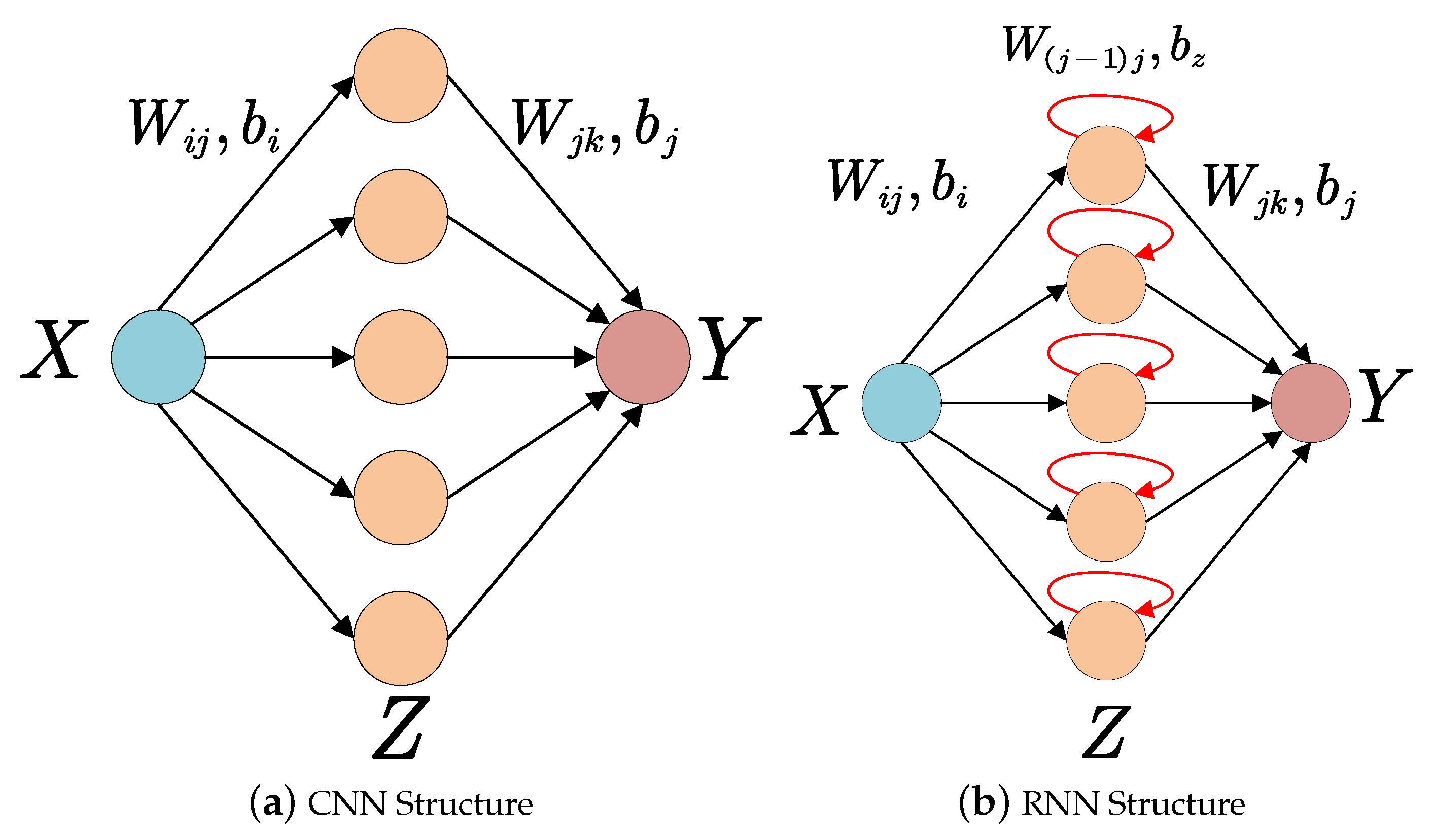
Table 1.
Performance comparison of state-of-the-art FPGA-based accelerator designs.
| Models | Quantization | Speed (GOPS) | Energy Efficiency (GOPS/W) | Platform |
|---|---|---|---|---|
| ESE [16] | 12b | 282.2 | 6.9 | XCKU060 |
| C-LSTM [17] | 16b | 131.1 | 6.0 | Virtex-7 |
| DeltaRNN [18] | 16b | 192.0 | 26.3 | XC7Z100 |
| BBS-LSTM [19] | 16b | 304.1 | 15.9 | Arria 10 GX1150 |
| Synetgy [20] | 4-4b | 47.09 | 8.56 | Zynq ZU3EG |
| DoReFa-Net [21] | 2b | 410.2 | 181.5 | ZC702 |
| XNOR-Net [22] | 1b | 207.8 | 44.2 | ZC702 |
Table 2.
Performance comparison of state-of-the-art FPGA-based accelerator designs.
| D.Han [28] | TPU-V2 | PDFA [29] | Eyeriss [30] | Envision [31] | UNPU [32] | Sticker [33] | SNAP [34] | |
|---|---|---|---|---|---|---|---|---|
| Technology (nm) | 65 | 20 | 65 | 65 | 28 | 65 | 65 | 16 |
| Frequency (MHz) | 200 | \ | 50–200 | 100–250 | 200 | 5–200 | 20–200 | 33–480 |
| Power (mW) | 126 | 225,000 | 168 | 235–332 | 7.5–300 | 3.2–297 | 20.5–248.4 | 16.3–364 |
| Data Width | INT13,16 | bfloat16 | INT13,16 | INT16 | INT1-16 | INT1-16 | INT8 | INT16 |
| Peak Throughput (GOPS) | 51.2 | 45,000 | 129.5 | 42.0 | 408 | 345.6 | 102–5638 | \ |
| Area (mm) | 3.52 | \ | 5.76 | 12.25 | 1.87 | 16 | 7.8 | 2.4 |
| Energy Efficiency (GOPS/W) | 406.4 | 200 | 770.8–1321 | 126.5 | 260–10,000 | 3080 | 411–62,100 | 21,550 |
Publisher’s Note: MDPI stays neutral with regard to jurisdictional claims in published maps and institutional affiliations. |
© 2021 by the authors. Licensee MDPI, Basel, Switzerland. This article is an open access article distributed under the terms and conditions of the Creative Commons Attribution (CC BY) license (https://creativecommons.org/licenses/by/4.0/).
Share and Cite
MDPI and ACS Style
Wu, R.; Guo, X.; Du, J.; Li, J. Accelerating Neural Network Inference on FPGA-Based Platforms—A Survey. Electronics 2021, 10, 1025. https://0-doi-org.brum.beds.ac.uk/10.3390/electronics10091025
AMA Style
Wu R, Guo X, Du J, Li J. Accelerating Neural Network Inference on FPGA-Based Platforms—A Survey. Electronics. 2021; 10(9):1025. https://0-doi-org.brum.beds.ac.uk/10.3390/electronics10091025
Chicago/Turabian StyleWu, Ran, Xinmin Guo, Jian Du, and Junbao Li. 2021. "Accelerating Neural Network Inference on FPGA-Based Platforms—A Survey" Electronics 10, no. 9: 1025. https://0-doi-org.brum.beds.ac.uk/10.3390/electronics10091025
Note that from the first issue of 2016, this journal uses article numbers instead of page numbers. See further details here.