
Ternary Neural Networks Based on on/off Memristors: Set-Up and Training
by
 , , , and
Antoni Morell
1,* ,
,
Elvis Díaz Machado
1,
Enrique Miranda
2,
Guillem Boquet
3 and
Jose Lopez Vicario
1 1
Departament de Telecomunicació i Enginyeria de Sistemes, Universitat Autònoma de Barcelona (UAB), 08193 Bellaterra, Spain
2
Departament d’Enginyeria Electrònica, Universitat Autònoma de Barcelona (UAB), 08193 Bellaterra, Spain
3
Wireless Networks (WiNe) Research Laboratory, Internet Interdisciplinary Institute (IN3), Universitat Oberta de Catalunya (UOC), 08860 Castelldefels, Spain
*
Author to whom correspondence should be addressed.
Electronics 2022, 11(10), 1526; https://0-doi-org.brum.beds.ac.uk/10.3390/electronics11101526
Submission received: 25 March 2022
/
Revised: 29 April 2022
/
Accepted: 3 May 2022
/
Published: 10 May 2022
(This article belongs to the Special Issue RRAM Devices: Multilevel State Control and Applications)
Abstract
:Neuromorphic systems based on hardware neural networks (HNNs) are expected to be an energy and time-efficient computing architecture for solving complex tasks. In this paper, we consider the implementation of deep neural networks (DNNs) using crossbar arrays of memristors. More specifically, we considered the case where such devices can be configured in just two states: the low-resistance state (LRS) and the high-resistance state (HRS). HNNs suffer from several non-idealities that need to be solved when mapping our software-based models. A clear example in memristor-based neural networks is conductance variability, which is inherent to resistive switching devices, so achieving good performance in an HNN largely depends on the development of reliable weight storage or, alternatively, mitigation techniques against weight uncertainty. In this manuscript, we provide guidelines for a system-level designer where we take into account several issues related to the set-up of the HNN, such as what the appropriate conductance value in the LRS is or the adaptive conversion of current outputs at one stage to input voltages for the next stage. A second contribution is the training of the system, which is performed via offline learning, and considering the hardware imperfections, which in this case are conductance fluctuations. Finally, the resulting inference system is tested in two well-known databases from MNIST, showing that is competitive in terms of classification performance against the software-based counterpart. Additional advice and insights on system tuning and expected performance are given throughout the paper.
1. Introduction
Neuromorphic computing, which imitates the principle behind biological synapses with a high degree of parallelism, has recently emerged as a very promising candidate for novel and sustainable computing technologies [1]. Among these technologies, neuromorphic systems based on hardware neural networks (HNNs) implemented with memristive devices have emerged as a promising solution for building energy-efficient computing frameworks for solving most of the tasks carried out in machine learning [2,3,4]. This is because memristors (1) behave as a resistor with memory that is electrically programmable and matches the functionality of the connections in a software neural network and (2) are efficiently integrated thanks to the crossbar array structure (i.e., aggressive size scaling is possible) [1,5,6].
Focusing on specific implementations that use memristors based on the crossbar array structure, it is worth noting first that this is one common approach found in the literature [7]. By using this structure, vector-matrix multiplications, which are a fundamental building block in all types of neural networks, are efficiently implemented by following an analog approach (i.e., by adding current flows). The efficiency of the operation is both in terms of (1) power consumption, because the involved currents are small, and (2) computational time [8], because the whole operation is performed by reading the outputs of the array. Note that a vector-matrix operation in software has a computational time that is and that individual memristors in the crossbar array play the role of the matrix coefficients or, in terms of neural networks, the weights. The interested reader can find in [9] a specific sound localization application based on memristor arrays. Energy consumption is reduced a factor of 184 with regard to the existing Application-Specific Integrated Circuit (ASIC) design.
Memristor-based networks can be trained by offline (or ex situ) or online (or in situ)-learning methods. In the first case, which is the focus of this manuscript, the weights are calculated on a precursor software-based network and then imported sequentially into the crossbar circuit. In the second case, training is implemented in situ in hardware and only for small neural networks [10], so the weights are adjusted in parallel, which is significantly more demanding [5]. In both cases, a high precision weight import is required to implement complex networks and achieve the expected performance when the network is operating. However, various properties of memristors are known to negatively affect the performance of neuromorphic systems [1]. Specifically, the conductance response of any real nonvolatile memory (NVM) device exhibits non-idealities that can surface in the form of unreliable performance of the network. Those imperfections include non-linearity, stochasticity, varying maxima, asymmetry between increasing and decreasing responses, and unresponsive devices at low or high conductance [11,12,13,14]. For example, most memristive devices exhibit a nonlinear weight update, where the conductance gradually saturates [1]. In addition, related to HNNs from the perspective of high-performance computing, recent trends show a growing interest in hardware that is capable of accelerating both training and inference in neural networks, especially when dealing with deep learning schemes. That is the case, for example, with many Field-Programmable Gate Array (FPGA) implementations [15], which emphasize the idea of quantized neural network designs due to the nature of FPGA devices. In particular, binary [16] and also ternary [17] implementations have been raised as very interesting options. The main motivation of this alternative approach is the reduction of both power consumption and the FPGA specs (required area). Memristor-based neural networks can also benefit from the power and area. However, the operational principles of memristors are completely different to those found in FPGAs, and at the end of the day, all HNN solutions require solving very specific challenges, as far as a straightforward conversion from the ideal (or software-based) model does not exist. As commented above, one of the challenges in memristor-based neural networks, which work from an analog perspective, is the development of reliable weight implementation due to the variability that is common to all nano-electronic devices but is significantly important in memristors [18].
In that direction, the authors of [4] stated that many issues still need to be resolved at the material, device, and system levels to simultaneously achieve high accuracy, low variability, high speed, energy efficiency, a small area, low cost, and good reliability. Thus, the first step is to obtain memristor-based networks that are competitive in comparison to software-based networks. In order to achieve that, we need to cope with the hardware. This can be accomplished at the hardware level with more advanced mitigation techniques or at the analgorithmic level by taking into account the non-idealities. In that sense, the authors of [10] presented a mask technique to capture the sneak path problem, stating that any kind of training incorporating the knowledge of the crossbar array behavior will likely improve the accuracy of memristor-based networks significantly. This idea was explored by several recent works following different strategies. In [19], for instance, a tailored training method was proposed to address the voltage drop due to the interconnected wire resistance. Basically, the voltage drop is estimated to recompute the weights at the forward propagation stage during the training procedure. In [20], the authors considered the mapping of neural network weights by analyzing the parasitic resistance effects at the different areas of the crossbar array. By identifying those hardware cells providing higher accuracy as “safe zones”, adaptive weight allocation was performed to properly map the weights to the hardware. In [21], the authors mathematically modeled the sensitivity of the output of the neural network with respect to hardware impairments. Then, the cost function of the training algorithm was adapted to consider this sensitivity as an additional term (i.e., the weights were calculated to minimize the impact of hardware impairments as well).
The aim of our work is also to consider hardware impairments during the design and training of the memristor-based neural network. To do so, we depart from software models that emulate the behavior of the memristor-based neural network. More specifically, this work is an extension of the work in [22], and we consider building ternary networks using crossbar arrays. The goal is to achieve performances close to the software models, even when we consider a simple configuration of the memristors operating like ON/OFF switches. It is worth noting that we adopt ternary weights because they have stronger expressive abilities than their binary counterpart [17]. As shown in Section 2, a ternary option does not modify the proposed crossbar array architecture, and the hardware remains the same (i.e., two conductance levels at the memristor weights).
The main contributions of this work are as follows:
- The behavior of a ternary memristor-based HNN adopting crossbar arrays is emulated;
- Practical configuration strategies to tune the crossbar array structure from a system-level designer point of view are proposed;
- An offline (ex situ) training mechanism is derived to optimize the neural network’s weights by minimizing the impact of conductance imperfections in the memristors’ hardware.
In what follows, Section 2 defines the problem under study, including the crossbar array architecture that we are considering to emulate ternary networks. Section 3 the encompasses configuration issues as well as the algorithm considered to fix the memristors to either the ON or the OFF status. Finally, Section 4 provides the experimental results, and Section 5 concludes the paper.
2. Scenario Description and Assumptions
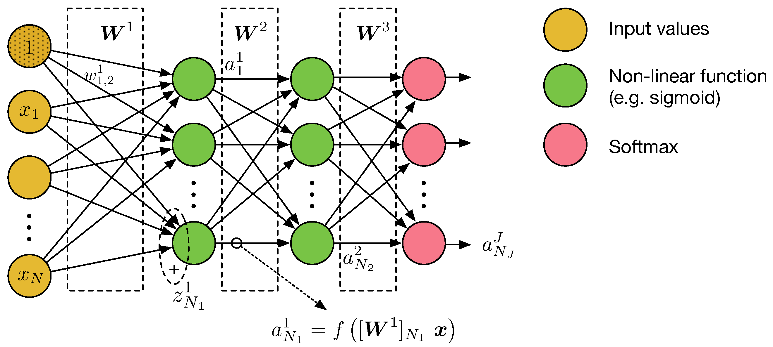
Let us consider a generic feedforward neural network (FFNN) that is dedicated to a classification task, as depicted in Figure 1. The network has inputs , where stands for the matrix transpose and the first input is manually set to 1 in order to accommodate the bias term. The FFNN operates as described next. First, the inputs are linearly combined by means of a matrix multiplication with , thus generating the values , i.e., (see Figure 1). Superindex 1 here stands for the first layer of the network. The values in go through a nonlinear function f (typically the sigmoid, the hyperbolic tangent or the rectified linear unit) to generate the activations at the first layer (i.e., with ). This process is repeated at the subsequent layers of the FFNN, such as the output at the second layer being computed from by first computing and then transforming the values in by using the non-linear function f again. Finally, at the last layer, also called the output layer, f is replaced by the softmax function. In this case, the output is normalized (i.e., ), and the value of indicates our confidence level in that corresponds to the ith class. Therefore, the network takes the output with largest value as the resulting classification.
All the operations described above are computed in floating-point arithmetic. We will refer to it as the software implementation. In this work, we employ the crossbar array to compute the vector-matrix multiplications at the neural network layers (i.e., ). Figure 2 depicts the operational principle of a crossbar array. Let us first consider the memristor in its linear zone, where it can be modeled simply as a resistor of conductance value g (adjustable) so that the memristor current is when the voltage v is applied. By scaling this to a crossbar of the size and arranging the conductance values in the matrix , we have with and (see Figure 2). In other words, the collected currents at the output of the crossbar array are in fact a vector-matrix multiplication between the input voltages and the memristor conductances in .
Let us briefly comment on the linearity of the memristor we are considering. According to the memdiode model [23], the I–V characteristic of a memristor reads as
where is an increasing function of the parameter (the memory state), R is the series resistance, and is a fitting parameter. Notice that Equation (1) is an implicit equation for the current I. Let us consider two extreme cases. The first is the high-resistance state (HRS) regime (with ). In this case, for low voltages, we have , and the potential drop across the series resistance can also be neglected such that
Second, for the low-resistance state (LRS) (with ), the difference is that the potential drop across R cannot be disregarded, and so
which can be solved as
The linear regime of the memristor corresponds to a case in between these two extreme situations so that the corresponding conductance reads as
which is independent of the voltage (i.e., it behaves as a simple resistor). This is the regime we are considering in our paper.
From an FFNN application point of view, the weights in in the software model are equivalent to the conductances in . Usually, both positive and negative weights are represented, even when we consider only two possible values as in binary neural networks [16]. We may add a third possible value, a zero, as in ternary networks so that a particular input or activation does not affect the net outputs. As shown below, this ternary option does not modify the proposed hardware architecture (based on two crossbar arrays), as the zero weight is built naturally by combining the same conductance levels with opposite polarization. We are also exploiting the advantage of having a higher granularity when compared with its binary counterpart, as proven in [17]. Note, however, that some differences between the software model (i.e., complementary metal–oxide–semiconductor (CMOS)-based) and the memristor-based model arise. We next list the considerations in this paper:
- We need to transform the output currents at the crossbar array to voltages by means of I-to-V converters. The scale factor of the I-to-V converters is defined as .
- The input voltages to the different layers shall be in the linear zone of the memristor (i.e., in the range ). Therefore, we need to scale both the inputs and the activations, because these are the inputs to the next network layers.
- We use the sigmoid as the nonlinear function f, which ranges from 0 to 1. Therefore, a scale factor of an amplitude equal to is required.
- Memristors are set to either LRS, where the conductance is set to , or HRS, where the conductance is set to (ON/OFF).
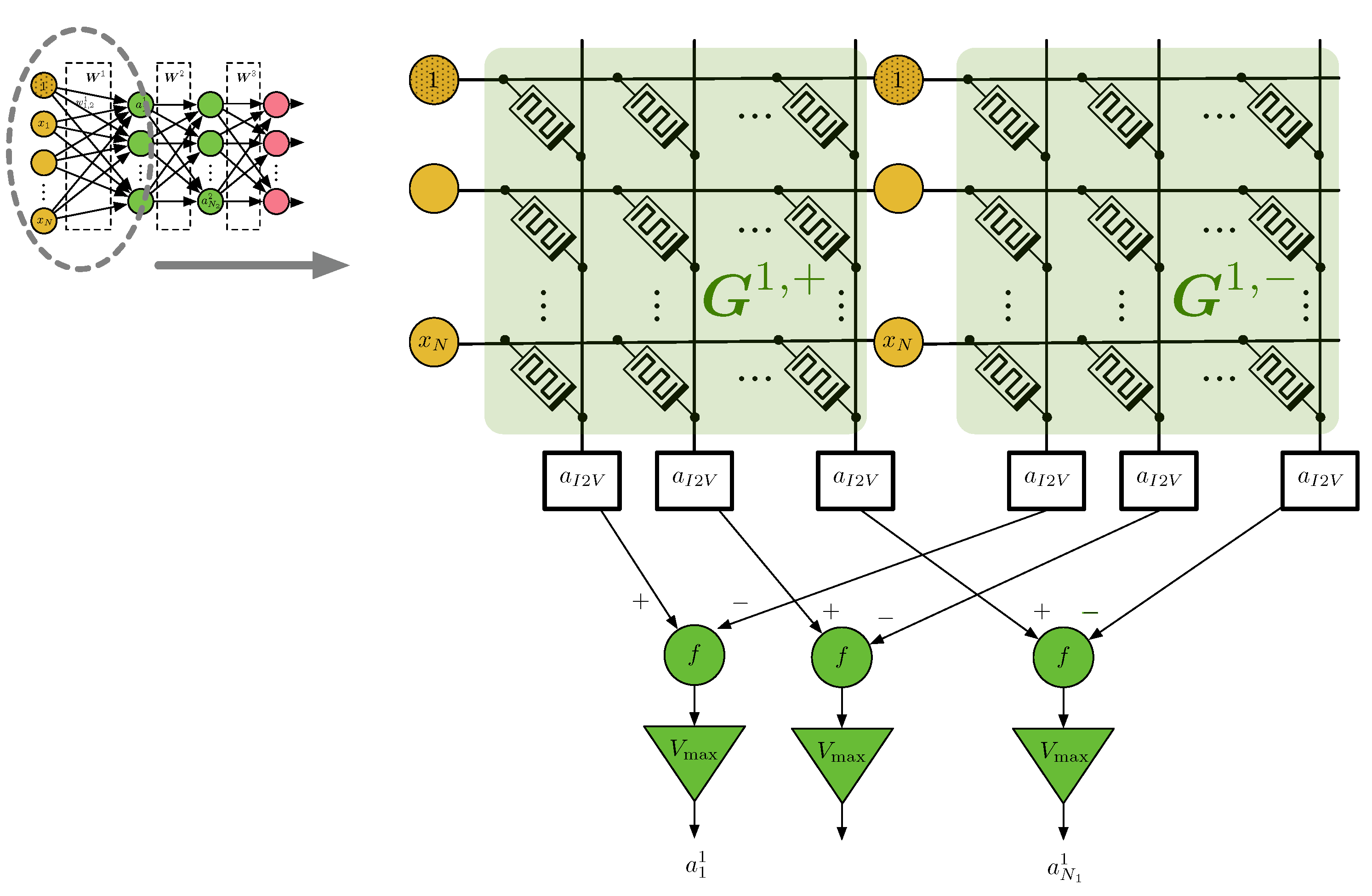
- Since the conductance values are strictly positive, a single crossbar array cannot emulate both positive and negative weights, as we have in the software model. To overcome this, we need a second crossbar array that considers the negative weights as depicted in Figure 3. Equivalently, the value of each weight in the software model is emulated by the combination , where the superindexes + and − distinguish the first and second crossbar arrays at the jth layer, respectively.
- The memristors are programmed ex situ; that is, we first compute in the software the weights of the memristor-based neural network (considering non-idealities), and once obtained, we fix the conductances in the memristors. From that moment on, the crossbar arrays remain unchanged.
- The memristors are programmed to either or , but the conductance values actually written add a random additive component. In particular, , where and . and represent the variances of the conductance in the HRS and LRS, respectively. We assume there are uncorrelated random additive components among the memristors.
- We consider to emulate the positive weight, say , to emulate the negative weight, say , and to emulate the null weight. Table 1 shows the set-up of the memristors in the positive and negative crossbar arrays and the corresponding weights. Alternatively, the null weight can be , too. Note that our first option reduces the current and thus the power consumption.
The goals in this work are the following:
- To adjust the conductance values in and (i.e., to decide which memristors are set to and which are set to );
- To adjust the value of , taking into account that memristors can be configured in the range . Note that all the memristors are programmed to the same value;
- To adjust the value of ;
- To consider conductance randomness in the training process.
Note that we consider devices operating in the linear regime (i.e., in the low-voltage region), and thus nonlinearities in the I–V characteristic can be disregarded [23]. Beyond this point, the conductance of the devices may change as we move to the programming region, which is out of the scope of this work. Aside from that, line resistance, which does not affect the linearity of the devices, may also be considered, and the synaptic weights probably need to be recalculated because of the parasitic potential drops. If the devices operate in the low-voltage regime and the array is not too large, these voltage drops can be disregarded as well. This ultimately depends on the integration technology.
The next section describes the algorithm developed for the ex situ training of the memristor-based FFNN.
3. Proposed Algorithm
In this section, we consider the equivalent software model in Figure 1 in order to train and configure our memristor-based FFNN, depicted in Figure 3.
3.1. Training of Quantized Neural Networks
Training of the resulting quantized neural network is accomplished using the so-called backpropagation algorithm as described in [16]. The idea is simple: the forward pass in the backpropagation applies the quantization, whereas the backward pass computes the gradients as usual in order to update the weights. Stochastic and efficient optimization is accomplished by randomly shuffling the data and by training consecutively on small subsets of the data, respectively. Algorithm 1 shows the steps of the training process.
| Algorithm 1 Algorithm for training a quantized network. |
| Input: Batch of training examples and labels Output: Initialization 1: Randomly initialize the weights at the J layers in the FFNN LOOP Process 2: for to do 3: for to do 4: (q is defined in Equation (6) below) 5: Forward propagation: compute network activations and outputs using 6: Backward propagation: use to compute gradients 7: 8: end for 9: end for 10: return |
3.2. Ternarization
We considered the following quantization function , which is defined as
We considered two options to fix . The first one was to set it to a fixed value. The second one was to try to optimize the value of according to the current weights at time t in so that was updated at each iteration of the algorithm. We followed the work in [17] to adjust the value of as
where is the all-ones column vector and is the total number of weights in the FFNN. The aim was to adapt the threshold to the current distribution of the weights. Note that is the same for all network layers in our work, although different thresholds per layer could also be considered.
3.3. Adaptation of
The proposed crossbar structure has two additional parameters to configure. Recall that we assumed an ON/OFF memristor model and that the conductances for the LRS and HRS were common to all memristors in the array. Notwithstanding, memristors can be programmed to different conductance values in the LRS. In this subsection, we develop the tuning of the conductance in . Recall that in Algorithm 1, we configured the memristors in our network to either the LRS or the HRS, relying on backpropagation. In particular, note that the unquantized weights that are written in the memristor network, as the LRS will generally differ from . In other words, usually we have
Therefore, we can use the values in to also update and reach a consensus value . Consider the following update rule:
where is the forgetting factor and is a masking function that operates element-wise in order to consider only the weights that have influence in (i.e., not the null weights). When is applied to a scalar in , say , it produces the following output:
Additionally, is the total number of weights whose quantization is different from zero at iteration .
However, note that a single weight in the neural network, say , once quantized, requires three elements in our hardware model to be represented: two memristors (one in and one in ) and an I-to-V converter. In other words, is represented in our physical model as . Furthermore, we set (assuming when ) in order to map the weights , as is the case in software-based ternary networks [17]. However, the conductance variance , which does not depend on the particular value of , now plays an important role, and the best choice is to set to the largest value allowed. Note that after division by in the I-to-V converter, the resulting conductance variance is also downsized.
In short, the discussion above is to point out that the best strategy is to set as large as possible and then fine-tune our memristor-based neural network by adjusting the gain in the I-to-V converter, as we show next.
3.4. Adaptation of
Let us consider that each output at the crossbar array could be adjusted separately (i.e., we have ). In this case, it is not complicated to compute the gradients for these parameters. It is similar to the weight gradients in backpropagation. For example, consider the scores , where ⊙ stands for the Hadamard product at the output layer of the neural network. If we train it using cross-entropy (assuming a classification task) (i.e., , where is the number of classes, (0 or 1) are the targets and are the network outputs), the gradients are found as follows:
where selects the ith row of matrix .
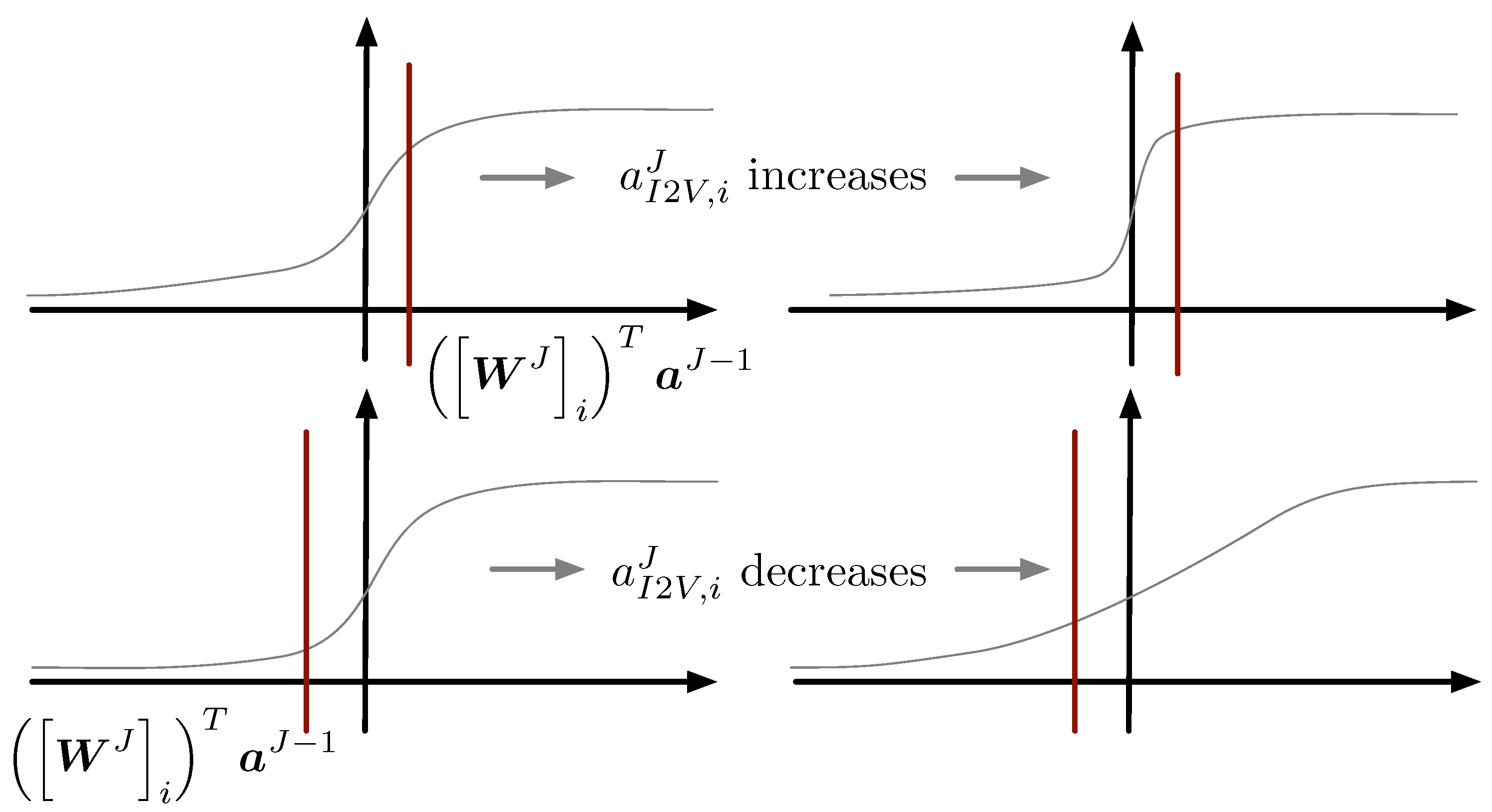
Let us analyze the effect of this gradient in the network, depicted in Figure 4. Assume that (so the current example belongs to the ith class). Unless we get a perfect classification, and the first term of the gradient will be negative. Therefore, if is positive (i.e., we are at the positive side of the sigmoid or softmax), the gradient is negative, and should be increased according to Equation (11). The effect is to shrink the sigmoid or softmax in order to increase the value of . If is negative, we are on the negative x-axis of the sigmoid or softmax, and the update of stretches the curve. This increases the value of and therefore diminishes the classification error. The reader can refer to Figure 4 for a graphical visualization of the discussion above. The analysis for is similar and not included here for the sake of brevity.
Having separate conversion gains at all crossbar outputs that are individually adapted is a real possibility. However, since we assume a common converter value, we must build a consensus gradient from all individual gradients such that
where (i.e., the total number of outputs in the J layers of the FFNN). We can now apply gradient-descent-based solutions to optimize .
Another option is to simply consider as a hyperparameter of the neural network (it is a scalar value) and optimize.
3.5. Including Robustness in Perturbed Conductances
The last issue we consider is the perturbation of the conductances that are written to the memristors; that is, we want to set the memristor to a conductance level or , but the level we actually achieve differs by a Gaussian perturbation term (zero-mean and variances and , respectively).
In order to cope with this physical impairment, we adopted an approach that resembles the training of quantized networks. Specifically, in the backward pass of backpropagation, we added a Gaussian term to the weights. The variance of that random contribution was set to , which is a hyperparameter of the network. In other words, we considered the following approach (in algorithmic style). This step substitutes step 7 in Algorithm 1.
The approach has a well-established foundation that connects to the regularization methods in neural networks. Primarily used in the context of recurrent neural networks, as described in [24] (Ch. 7.5), noise injection (i.e., adding random values to the weights) adds robustness to the network in the sense that the model learned is somehow insensitive to small variations in the weights. In other words, our approach can be interpreted as a form of regularization.
4. Experimental Results
In this section, we experimented with the proposed ternary network in order to evaluate the effects of the different adaptation mechanisms (conductance at the LRS and the conversion factor at the I-to-V stage), as well as the effect of quantizing the weights and the incorporation of weight variability during training. We considered two different datasets widely employed as benchmark datasets in machine learning: the Modified National Institute of Standards and Technology(MNIST) dataset [25] and the fashion MNIST dataset [26]. Both datasets consist of grayscale images of 28 × 28 pixels. The former contains images of handwritten numbers (from 0 to 9), whereas the latter also contains also different types (or classes) of images all related to clothes (e.g., t-shirts, pullovers or sandals, among others). In both cases, an 80–20 random split for training and testing was conducted.
In terms of neural network architecture, we considered an FFNN with two hidden layers of a size 1000 units/neurons. Taking into account 784 (=28 × 28) values at the input layer and 10 output classes, the whole architecture was 784–1000–1000–10, with a total of 7.85 G weights/parameters to be trained (including bias terms) in a full-software implementation and 15.7 G memristors to be set at either the LRS or HRS in the memristor-based neural network implementation. Training and evaluation were performed by means of Python programming using the Tensorflow library for deep neural networks [27]. The memristors were modelled in Python and Tensorflow according to the assumptions in Section 2.
Table 2 summarizes the electrical parameters considered in our experiments. We considered values that were in agreement with the state of the art of the memristive technology [10,28], but we also took into account larger conductance deviations in order to accommodate other fabrication technologies. Our goal here was to test the practical importance of synthesizing reliable devices in terms of conductance fluctuations. The conductance values are always relative to , the quantum conductance.
Finally, ternarization was applied with the adaptive threshold in Equation (7), and the performance metric employed was classification accuracy, which measured the number of examples (images in this case) correctly classified with respect to the total number of images (i.e., it was the percentage of images correctly classified).
4.1. Adaptation of
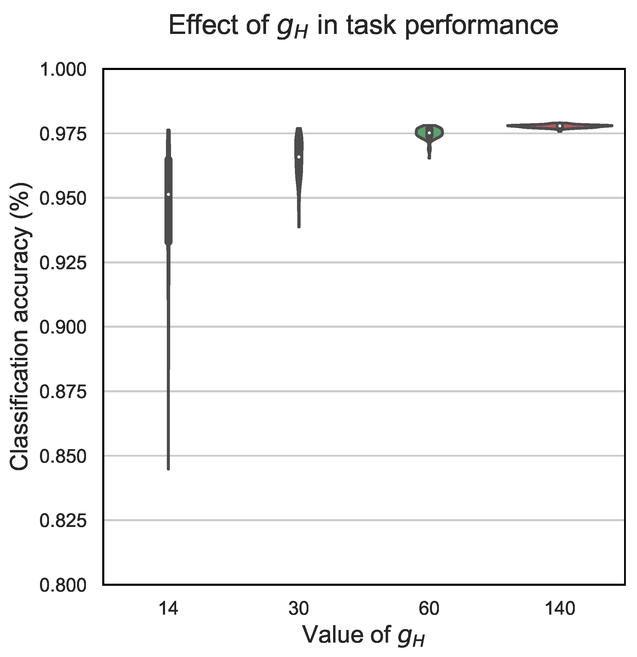
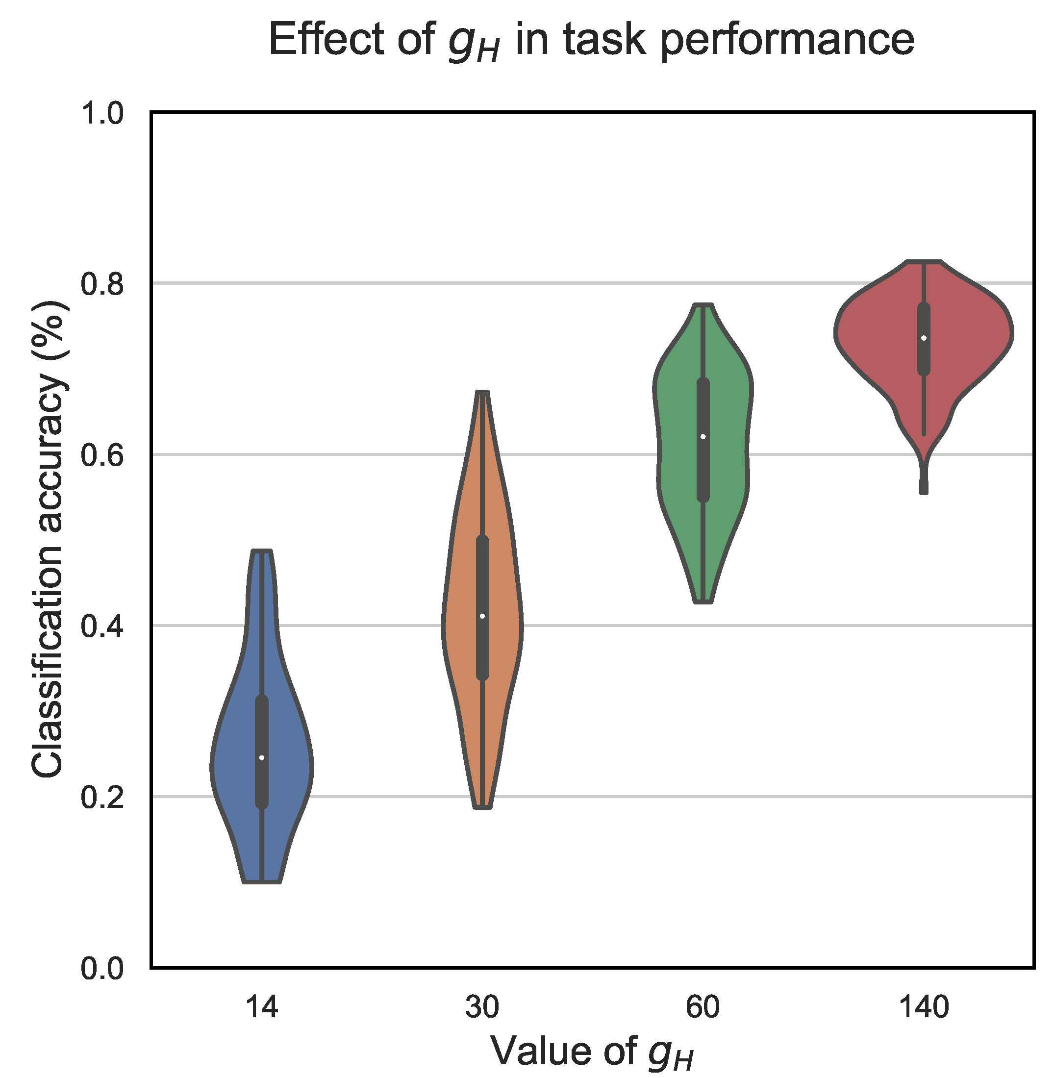
Our first experiment dealt with the adjustment of the conductance value for the LRS (i.e., ). In Figure 5 and Figure 6, we considered violin plots that showed the distribution of accuracies obtained after 1000 realizations. Remember that memristor conductances incorporate a random term (i.e., and ). Although the weights computed during training remained unchanged, their mapping to memristor conductances changed from one realization to another due to the random term. That aside, we considered here , the threshold used for the ternarization of the weights set as in Equation (7), and . Figure 5 considers , and Figure 6 considers .
As we can appreciate in Figure 5, where the conductance perturbations were moderate, the average accuracy was above 95% with all the tested adjustments of . However, the distribution of accuracy values was spread out significantly more for the case (ranging from 0.845 to 0.976), whereas the dispersion diminished for the case of (ranging from 0.939 to 0.977) and practically vanished for (ranging from 0.965 to 0.978) and more notably for (ranging from 0.976 to 0.979).
Figure 6 involves experiments with a severe conductance perturbation. In this case, the classification task was more complex, and with equal network configuration, the performance dropped. We appreciated the dispersion in the accuracy distributions for all cases of , although the dispersion tended to reduce as increased. In this best case, the accuracy ranged from 0.551 to 0.825, so the difference between the max and min value was 0.274. In this application, it is important to note the mean values for the accuracy. For the two lowest conductance values, the mean accuracy was 25.8% for and 41.9% for . This value grew up to 61.1% for and to 73% for .
In conclusion, both experiments confirmed that should be adjusted to the highest possible value (depending on the available technology) in order to achieve the best possible performance.
4.2. Adaptation of and Robustness to Perturbed Conductance Values
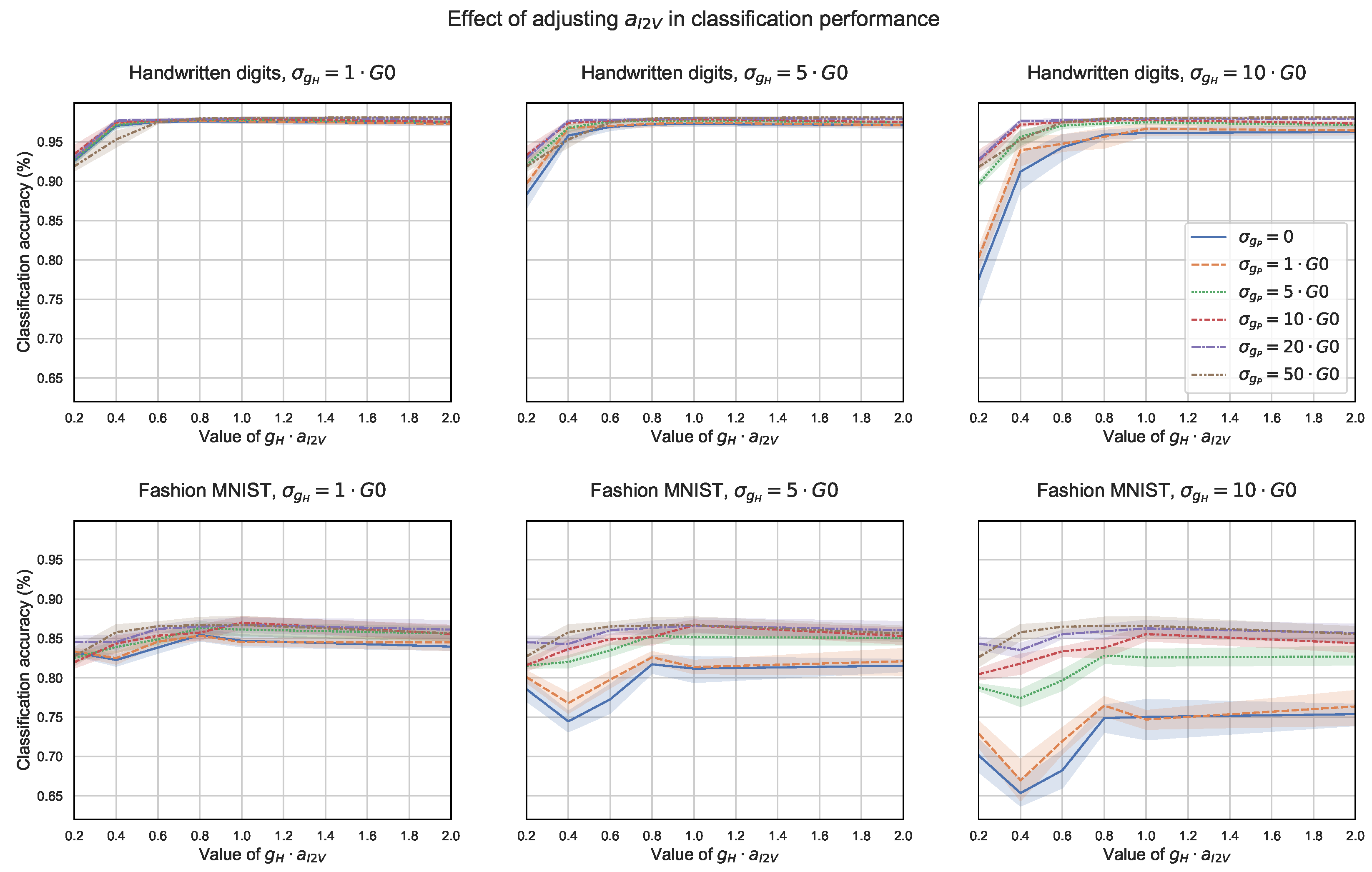
In Figure 7, we tested how sensitive the classification accuracy was to adjustment of the value in and to the weight perturbance introduced during training (i.e., ), assuming . We considered both datasets under study (handwritten digits and fashion MNIST), and we plotted the classification accuracy as a function of , testing different combinations of and , particularly and . As we can appreciate in the figure, setting (i.e., ) gave us a particularly good initial adjustment. In the applications tested, the plots show that the performance could be just slightly increased by choosing the optimal value of , as long as the sensitivity around the initial adjustment was low. Note that the perturbance introduced during training (i.e., the value in ) had a larger influence on the classification accuracy (i.e., the different accuracy curves became more separated), especially for the fashion MNIST dataset when and . Note also that in general, the higher was, the more variation in performance we observed. As a rule of thumb, setting to a value in the range provided a proper adjustment.
4.3. Comparison with the Software-Based Neural Network
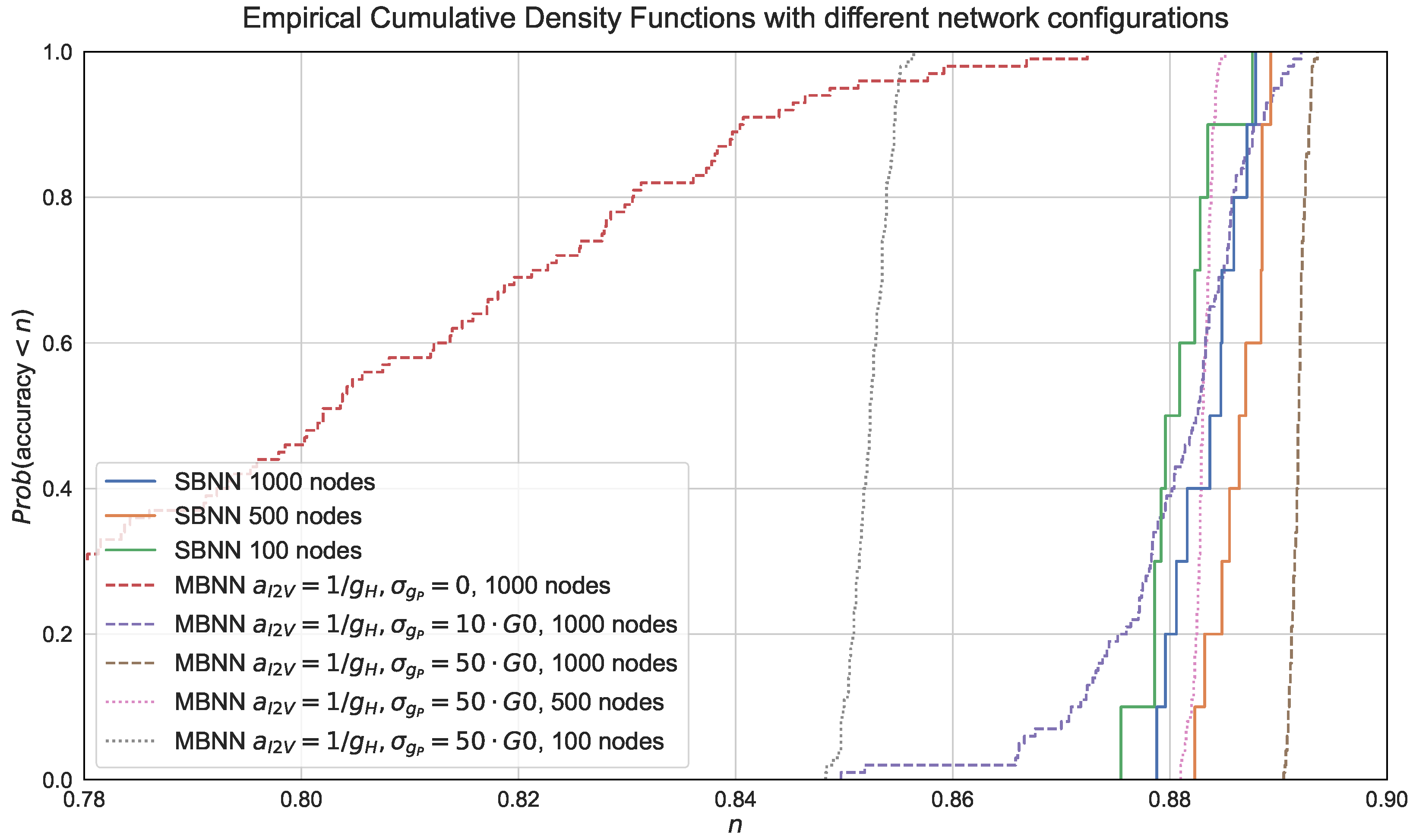
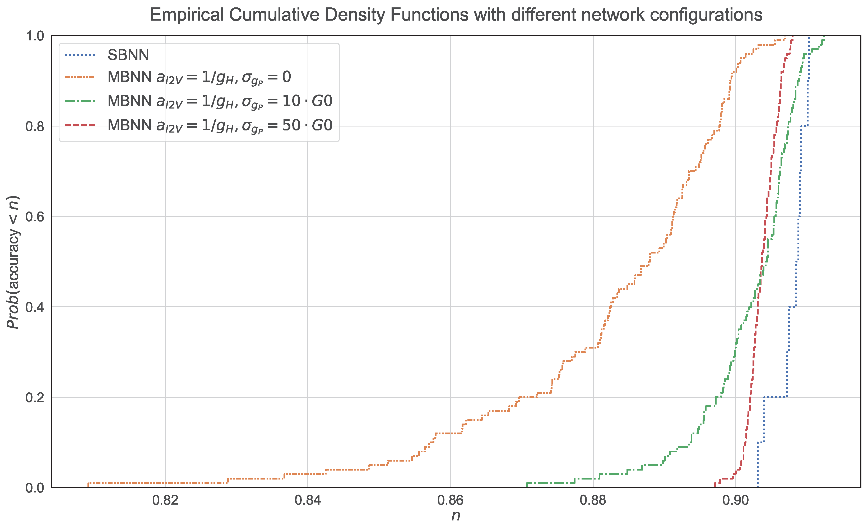
We then tested how a memristor-based neural network (MBNN) compared to a software-based neural network (SBNN). For this occasion, we took into account ternarization of the weights as well as mitigation of the conductance perturbations and optimization of . Aside from the reference network architecture (i.e., 784–1000–1000–10), we also considered 784–500–500–10 and 784–100–100–10 for the MBNN and SBNN models. The results reported the empirical cumulative density functions (ecdf). Note that the SBNN suffered no perturbation once the weights were fixed, but the performance slightly varied due to the random initialization of weights in training, too. In order to reflect this issue, we then considered 1000 realizations in total for each model containing 10 different training processes. In other words, the same set of weights was used to perform 100 inferences. Note that in the SBNN, all inferences that used the same set of weights produced the same results, whereas in the MBNN, this was not the case due to conductance fluctuations. We considered here the classification of the fashion MNIST dataset, which is a more complex task than handwritten digit classification, assuming and .
In Figure 8, we next compare the following methods: (1) SBNNs with 1000, 500 and 100 units in the two hidden layers; (2) an MBNN (1000 units in the hidden layers) with , (i.e., we did not consider conductance fluctuations in training), an MBNN with , (i.e., a default set-up assuming fluctuations in training) and a fine-tuned MBNN (in this case requires increasing to ); and (3) the fine-tuned MBNN version with 500 and 100 units in the hidden layers.
The results essentially show two issues when we considered 1000 units at each hidden layer. First of all, there was the importance of considering memristor fluctuations during training. Note the spreading in the ecdf for , which had a maximum value of 0.8724 and a minimum value of 0.6274 (i.e., the gap was 0.245). This gap significantly reduced to 0.042 in the case of the default set-up and practically vanished in the tuned MBNN and also the SBNN. Second, a properly tuned MBNN achieved a performance that was similar to the SBNN counterpart. If we look at the worst performance in all the set-ups, the SBNN archived an accuracy of 0.8788, the MBNN with yielded 0.6274 (a 28.6% reduction with respect to the SBNN), and the MBNN with obtained 0.8905 (a 1.3% increase with respect to the SBNN). This slightly better performance might have been due to the regularization effect produced when we included robustness to perturbed conductance values by means of . For the cases of 500 and 100 hidden units per layer, the MBNN performed close the SBNN for 500 units and suffered a reduction of about 3% in accuracy for the case with 100 hidden units. Therefore, weight quantization affected the performance more as the complexity of the model was further constrained.
4.4. Summary and Extension of Results
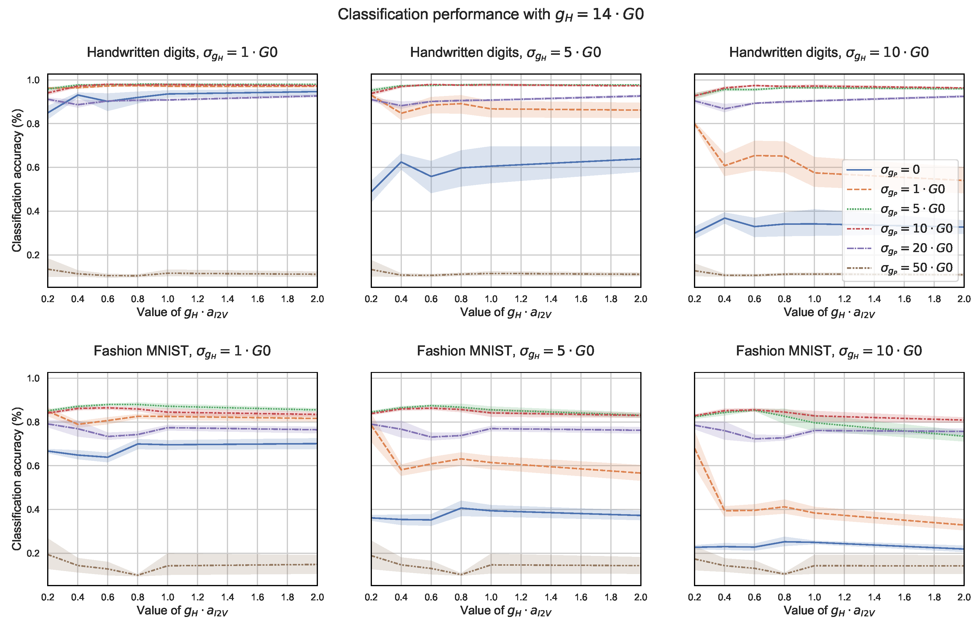
To summarize the results so far, we saw that the performance in general depended on the task complexity, the network configuration as well as on the memristor quality, where the larger the and the lower the , the better. Regarding task complexity, Figure 7 plots the results of the exact same models applied to two different tasks. In the top row, the less complex task showed less variability among models such that a proper adjustment of was less critical. In the bottom row, the more complex task showed more variability and required a good adjustment of . In order to complete our analysis, now with a lower quality memristor, we could reproduce in Figure 9 the same experiments while considering instead of . As we can appreciate in the figure, the classification accuracy in the different models was far more sensitive to the proper adjustment of . The worst performing models in the classification of handwritten digits (top row) then achieved accuracies around or below 20%, whereas the worst accuracy in Figure 7 was above 75%. Something similar occurred in the classification of clothes; the worst performing models achieved values around 20% whereas in Figure 7, the worst performance was above 65%.
Finally, we tested our memristor-based solution as part of a convolutional neural network (CNN) implementation applied to the classification of the fashion MNIST dataset. The input in this case was grayscale images of 28 × 28 pixels (i.e., 2D data). The configuration of our CNN was as follows:
- 2D convolutional layer with 32 filters, 3 × 3 kernels and rectified linear unit (ReLU) activation;
- 2D max pooling 2 × 2 layer;
- 2D convolutional layer with 64 filters, 3 × 3 kernels and ReLU activation;
- 2D max pooling 2 × 2 layer;
- 2D convolutional layer with 128 filters, 3 × 3 kernels and ReLU activation;
- Flatten layer (1152 values at output);
- Fully connected layer (1000 values at output);
- Fully connected layer (1000 values at output);
- Fully connected layer (10 values at the output to identify each of the 10 classes in the dataset).
Convolutional, max pooling and flatten layers were implemented in the software. This first block transformed each image into 1152 positive values at the output of the flatten layer (1D). The second block embraced the fully connected layers and was identical to the FFNN tested so far, except for the number of input values (768 before vs. 1152 now). This second block was implemented both in the software and using the proposed memristor-based neural network. In the latter case, the outputs at the flatten layer were scaled to fit the range . Note that the memristors could also be considered in the first block, but this introduces additional complexity in so far as more peripheral circuitry is required. This point is beyond the scope of the paper. In Figure 10, we reproduced the results in Figure 8 using the described CNN approach.
The results show that the performance, in terms of prediction accuracy, increased for all the configurations tested with respect to the FFNN approach. This was due to the high-level features processed at the convolutional and max pooling layers. The second observation is that increasing the value of gave robustness to the system (i.e., the accuracy values were less spread out). This result is coherent with the results obtained so far. Finally, we observed that the MBNN with a proper configuration was close in performance to the SBNN. These preliminary results encourage us to explore the application of memristors to more complex neural network architectures.
5. Conclusions
In this paper, we analyzed the implementation of deep neural networks using crossbar arrays of memristors, and more specifically, we considered the case where these devices can be configured in only two different states: a low-resistance state (LRS) and a high-resistance state (HRS). The natural usage of crossbar arrays in the context of neural networks is in performing vector-matrix multiplications in an analog fashion (i.e., by adding currents), thus reducing the power consumption and computational time. Our approach aims at emulating ternary neural networks, which sets the weights in the neural network to a value in the range of . In order to achieve this behavior, we need to implement two crossbar arrays for each feedforward layer in the network (i.e., one to represent the positive weights and the other one to represent the negative weights). Additionally, some other adaptation issues in relation to software-based neural networks arise: (1) the currents at the output of the crossbar arrays have to be converted to voltages for the next stage, resulting in a conversion factor that can be potentially tuned to boost network performance and (2) memristor device experiment conductance fluctuations that also impinge on performance. Taking these issues into account, we designed an algorithm to train the weights in the network and later map these weights to the network, where memristors are programmed to either the LRS or the HRS.
The results show that the proposed system design and offline training method represent a real alternative to the traditional software-based (i.e., CMOS-based) neural networks. The lessons learned in this work are as follows: (1) the higher the conductance of the memristor in the LRS, the better performance we can achieve; (2) the conversion factor that maps the output currents at one layer to input voltages at the next layer can be fine-tuned, but it is not a sensitive parameter; and (3) it is very important to consider mitigation of the conductance variability, as performance is very sensitive to this. In our experiments, we achieved accuracies that were similar to the software-based counterpart, but without considering conductance variability during training, we observed large gaps in terms of classification accuracy between the worst realizations. This gap could be above 50% in the 10-class classification tasks (handwritten digits and fashion MNIST data) we tested.
Future work could consider additional hardware issues such as nonlinearity, stochasticity, varying maxima, asymmetry between increasing and decreasing responses, non-responsive devices at low or high conductance, mixed time-varying delays or the sneak-path problem in crossbar arrays [10,11,12,13,14]. We also need to evaluate the performance using more complex and widely used neural network models, such as convolutional or recurrent networks. The preliminary results have been presented for a CNN here, showing the potential of memristor-based approaches.
Author Contributions
Conceptualization, A.M. and J.L.V.; methodology, A.M., J.L.V., E.D.M. and G.B.; software, E.D.M. and G.B.; validation, A.M., J.L.V. and E.M.; formal analysis, A.M. and E.M.; investigation, A.M., G.B., E.D.M. and J.L.V.; resources, A.M., J.L.V. and E.M.; data curation, E.D.M.; writing—original draft preparation, A.M. and J.L.V.; writing—review and editing, A.M., J.L.V. and E.M.; visualization, A.M. and E.D.M.; supervision, A.M., J.L.V. and E.M.; project administration, A.M. and J.L.V.; funding acquisition, A.M. and E.M. All authors have read and agreed to the published version of the manuscript.
Funding
This work is supported by the Spanish Government under Project TEC2017-84321-C4-4-R co-funded with European Union ERDF funds and also by the Catalan Government under Project 2017 SGR 1670.
Institutional Review Board Statement
Not applicable.
Informed Consent Statement
Not applicable.
Data Availability Statement
The MNIST and Fashion MNIST datasets used in this work are publicly available and can be obtained from http://yann.lecun.com/exdb/mnist/ (accessed on 2 May 2022) and https://github.com/zalandoresearch/fashion-mnist (accessed on 2 May 2022), respectively.
Conflicts of Interest
The authors declare no conflict of interest.
References
- Choi, S.; Ham, S.; Wang, G. Memristor synapses for neuromorphic computing. In Memristors-Circuits and Applications of Memristor Devices; IntechOpen: London, UK, 2020. [Google Scholar]
- Thomas, A. Memristor-based neural networks. J. Phys. Appl. Phys. 2013, 46, 93001. [Google Scholar] [CrossRef] [Green Version]
- Li, C.; Belkin, D.; Li, Y.; Yan, P.; Hu, M.; Ge, N.; Jiang, H.; Montgomery, E.; Lin, P.; Wang, Z.; et al. Efficient and self-adaptive in-situ learning in multilayer memristor neural networks. Nat. Commun. 2018, 9, 1–8. [Google Scholar] [CrossRef] [PubMed] [Green Version]
- Miranda, E.; Suñé, J. Memristors for Neuromorphic Circuits and Artificial Intelligence Applications. Materials 2020, 13, 938. [Google Scholar] [CrossRef] [PubMed] [Green Version]
- Alibart, F.; Zamanidoost, E.; Strukov, D.B. Pattern classification by memristive crossbar circuits using ex situ and in situ training. Nat. Commun. 2013, 4, 1–7. [Google Scholar] [CrossRef] [PubMed] [Green Version]
- Kim, H.; Mahmoodi, M.R.; Nili, H.; Strukov, D.B. 4K-memristor analog-grade passive crossbar circuit. Nat. Commun. 2021, 12, 1–11. [Google Scholar] [CrossRef] [PubMed]
- Huang, A.; Zhang, X.; Li, R.; Chi, Y. Memristor neural network design. In Memristor and Memristive Neural Networks; James, A.P., Ed.; IntechOpen: Rijeka, Croatia, 2018; Chapter 12. [Google Scholar] [CrossRef] [Green Version]
- Yuan, G.; Ma, X.; Ding, C.; Lin, S.; Zhang, T.; Jalali, Z.S.; Zhao, Y.; Li, J.; Soundarajan, S.; Wang, Y. An Ultra-Efficient Memristor-Based DNN Framework with Structured Weight Pruning and Quantization Using ADMM. In Proceedings of the 2019 IEEE/ACM International Symposium on Low Power Electronics and Design (ISLPED), Lausanne, Switzerland, 29–31 July 2019; pp. 1–6. [Google Scholar] [CrossRef] [Green Version]
- Gao, B.; Zhou, Y.; Zhang, Q.; Zhang, S.; Yao, P.; Xi, Y.; Liu, Q.; Zhao, M.; Zhang, W.; Liu, Z.; et al. Memristor-based analogue computing for brain-inspired sound localization with in situ training. Nat. Commun. 2022, 13, 2026. [Google Scholar] [CrossRef] [PubMed]
- Fouda, M.E.; Lee, S.; Lee, J.; Eltawil, A.; Kurdahi, F. Mask Technique for Fast and Efficient Training of Binary Resistive Crossbar Arrays. IEEE Trans. Nanotechnol. 2019, 18, 704–716. [Google Scholar] [CrossRef]
- Burr, G.W.; Shelby, R.M.; Sidler, S.; Di Nolfo, C.; Jang, J.; Boybat, I.; Shenoy, R.S.; Narayanan, P.; Virwani, K.; Giacometti, E.U.; et al. Experimental demonstration and tolerancing of a large-scale neural network (165,000 synapses) using phase-change memory as the synaptic weight element. IEEE Trans. Electron Devices 2015, 62, 3498–3507. [Google Scholar] [CrossRef]
- Pedro, M.; Martin-Martinez, J.; Rodriguez, R.; Gonzalez, M.; Campabadal, F.; Nafria, M. A flexible characterization methodology of RRAM: Application to the modeling of the conductivity changes as synaptic weight updates. Solid-State Electron. 2019, 159, 57–62. [Google Scholar] [CrossRef]
- Veksler, D.; Bersuker, G.; Vandelli, L.; Padovani, A.; Larcher, L.; Muraviev, A.; Chakrabarti, B.; Vogel, E.; Gilmer, D.C.; Kirsch, P.D. Random telegraph noise (RTN) in scaled RRAM devices. In Proceedings of the 2013 IEEE International Reliability Physics Symposium (IRPS), Monterey, CA, USA, 14–18 April 2013. [Google Scholar] [CrossRef]
- Vadivel, R.; Ali, M.S.; Joo, Y.H. Robust H-infinity performance for discrete time T-S fuzzy switched memristive stochasticneural networks with mixed time-varying delays. J. Exp. Theor. Artif. Intell. 2021, 33, 79–107. [Google Scholar] [CrossRef]
- Zhang, C.; Li, P.; Sun, G.; Guan, Y.; Xiao, B.; Cong, J. Optimizing FPGA-based accelerator design for deep convolutional neural networks. In Proceedings of the 2015 ACM/SIGDA International Symposium on Field-Programmable Gate Arrays, Monterey, CA, USA, 22–24 February 2015; Association for Computing Machinery: New York, NY, USA, 2015; pp. 161–170. [Google Scholar] [CrossRef]
- Simons, T.; Lee, D.J. A review of binarized neural networks. Electronics 2019, 8, 661. [Google Scholar] [CrossRef] [Green Version]
- Li, F.; Zhang, B.; Liu, B. Ternary weight networks. arXiv 2016, arXiv:1605.04711. [Google Scholar]
- Kim, S.; Kim, H.D.; Choi, S.J. Impact of Synaptic Device Variations on Classification Accuracy in a Binarized Neural Network. Sci. Rep. 2019, 9, 1–7. [Google Scholar] [CrossRef] [PubMed]
- Fouda, M.E.; Lee, S.; Lee, J.; Kim, G.H.; Kurdahi, F.; Eltawi, A.M. IR-QNN Framework: An IR Drop-Aware Offline Training of Quantized Crossbar Arrays. IEEE Access 2020, 8, 228392–228408. [Google Scholar] [CrossRef]
- Zhao, X.; Liu, L.; Si, L.; Pan, K.; Sun, H.; Zheng, N. Adaptive Weight Mapping Strategy to Address the Parasitic Effects for ReRAM-based Neural Networks. In Proceedings of the 2021 IEEE 14th International Conference on ASIC (ASICON), Kunming, China, 26–29 October 2021; pp. 1–4. [Google Scholar]
- Vahdat, S.; Kamal, M.; Afzali-Kusha, A.; Pedram, M. Reliability Enhancement of Inverter-Based Memristor Crossbar Neural Networks Using Mathematical Analysis of Circuit Non-Idealities. IEEE Trans. Circuits Syst. 2021, 68, 4310–4323. [Google Scholar] [CrossRef]
- Boquet, G.; Macias, E.; Morell, A.; Serrano, J.; Miranda, E.; Vicario, J.L. Offline training for memristor-based neural networks. In Proceedings of the 28th European Signal Processing Conference (EUSIPCO2020), Amsterdam, The Netherlands, 18–22 January 2021. [Google Scholar]
- Aguirre, F.L.; Suñé, J.; Miranda, E. SPICE Implementation of the Dynamic Memdiode Model for Bipolar Resistive Switching Devices. Micromachines 2022, 13, 330. [Google Scholar] [CrossRef] [PubMed]
- Goodfellow, I.; Bengio, Y.; Courville, A. Deep Learning; The MIT Press: Cambridge, MA, USA, 2016. [Google Scholar]
- Deng, L. The mnist database of handwritten digit images for machine learning research. IEEE Signal Process. Mag. 2012, 29, 141–142. [Google Scholar] [CrossRef]
- Xiao, H.; Rasul, K.; Vollgraf, R. Fashion-MNIST: A Novel Image Dataset for Benchmarking Machine Learning Algorithms. arXiv 2017, arXiv:cs.LG/1708.07747. [Google Scholar]
- Abadi, M.; Agarwal, A.; Barham, P.; Brevdo, E.; Chen, Z.; Citro, C.; Corrado, G.S.; Davis, A.; Dean, J.; Devin, M.; et al. TensorFlow: Large-Scale Machine Learning on Heterogeneous Systems. 2015. Available online: https://research.google/pubs/pub45166/ (accessed on 17 December 2021).
- Prakash, A.; Park, J.; Song, J.; Lim, S.; Park, J.; Woo, J.; Cha, E.; Hwang, H. Multi-state resistance switching and variability analysis of HfO x based RRAM for ultra-high density memory applications. In Proceedings of the 2015 International Symposium on Next-Generation Electronics (ISNE), Taipei, Taiwan, 4–6 May 2015; pp. 1–2. [Google Scholar]
Figure 1.
Feedforward neural network. represents the matrix multiplication of the last row in with the column vector , which includes all the input values plus the ‘1’ to accommodate the bias term.
Figure 1.
Feedforward neural network. represents the matrix multiplication of the last row in with the column vector , which includes all the input values plus the ‘1’ to accommodate the bias term.

Figure 2.
Crossbar array as a matrix multiplication.

Figure 3.
Implementation of an FFNN using crossbar arrays.

Figure 4.
Effect of adapting on the sigmoid.

Figure 5.
MNIST handwritten digit classification accuracy as a function of the value of . Conductance fluctuations are .
Figure 5.
MNIST handwritten digit classification accuracy as a function of the value of . Conductance fluctuations are .

Figure 6.
MNIST fashion classification accuracy as a function of the value of . Conductance fluctuations are .
Figure 6.
MNIST fashion classification accuracy as a function of the value of . Conductance fluctuations are .

Figure 7.
Classification accuracy as a function of the value of and for .

Figure 8.
Performance of SBNN and MBNN with different configurations in the classification of fashion MNIST data.
Figure 8.
Performance of SBNN and MBNN with different configurations in the classification of fashion MNIST data.

Figure 9.
Performance in the classification of handwritten digits and fashion MNIST data using memristors with .
Figure 9.
Performance in the classification of handwritten digits and fashion MNIST data using memristors with .

Figure 10.
Performance of the SBNN and MBNN with different configurations in the classification of fashion MNIST, using the CNN approach.
Figure 10.
Performance of the SBNN and MBNN with different configurations in the classification of fashion MNIST, using the CNN approach.


Table 1.
Set-up of memristors in and and corresponding ternary weights.
| Ternary Weight | ||
|---|---|---|
| 0 | ||
Table 2.
Electrical parameters in the memristor-based neural network.
| Parameter | Value or Range |
|---|---|
| 0.2 V | |
| 1 | |
| [14, 140] | |
| 1 | |
| 1–10 |
Publisher’s Note: MDPI stays neutral with regard to jurisdictional claims in published maps and institutional affiliations. |
© 2022 by the authors. Licensee MDPI, Basel, Switzerland. This article is an open access article distributed under the terms and conditions of the Creative Commons Attribution (CC BY) license (https://creativecommons.org/licenses/by/4.0/).
Share and Cite
MDPI and ACS Style
Morell, A.; Machado, E.D.; Miranda, E.; Boquet, G.; Vicario, J.L. Ternary Neural Networks Based on on/off Memristors: Set-Up and Training. Electronics 2022, 11, 1526. https://0-doi-org.brum.beds.ac.uk/10.3390/electronics11101526
AMA Style
Morell A, Machado ED, Miranda E, Boquet G, Vicario JL. Ternary Neural Networks Based on on/off Memristors: Set-Up and Training. Electronics. 2022; 11(10):1526. https://0-doi-org.brum.beds.ac.uk/10.3390/electronics11101526
Chicago/Turabian StyleMorell, Antoni, Elvis Díaz Machado, Enrique Miranda, Guillem Boquet, and Jose Lopez Vicario. 2022. "Ternary Neural Networks Based on on/off Memristors: Set-Up and Training" Electronics 11, no. 10: 1526. https://0-doi-org.brum.beds.ac.uk/10.3390/electronics11101526
Note that from the first issue of 2016, this journal uses article numbers instead of page numbers. See further details here.