
Energy Management Strategies for Hybrid Energy Storage Systems Based on Filter Control: Analysis and Comparison


1
Department of Electrical and Electronic Engineering, Universidad Nacional de Colombia, Bogotá 111321, Colombia
2
Departament d’Enginyeria de Sistemes, Automàtica i Informàtica Industrial (ESAII), Universitat Politècnica de Catalunya (UPC), 08028 Barcelona, Spain
*
Author to whom correspondence should be addressed.
Electronics 2022, 11(10), 1631; https://0-doi-org.brum.beds.ac.uk/10.3390/electronics11101631
Submission received: 11 April 2022
/
Revised: 6 May 2022
/
Accepted: 17 May 2022
/
Published: 20 May 2022
(This article belongs to the Section Systems & Control Engineering)
Abstract
:The Filter-Based Method (FBM) is one of the most simple and effective approaches for energy management in hybrid energy storage systems (HESS) composed of batteries and supercapacitors (SC). The FBM has evolved from its conventional form in such a manner that more flexibility and functionalities have been added. A comparative study and analysis of the most recent and relevant proposals based on the FBM for HESS are provided in this paper. In this way, the improvements for this energy management system (EMS) are in the form of adaptive filters, rules, Fuzzy logic control, sharing coefficients, and additional control loops. It is shown how these enhancements seek to avoid the premature degradation of the storage devices that are caused by deep discharge, overcharge, and fast current variations in the case of batteries and overcharge in the SC case. Therefore, the enhancements are focused on keeping the battery and SC working within safe operational limits. This paper presents new comparisons regarding the SoC evolution in the storage devices, specifically how the SC SoC is used in the EMS to establish the power sharing. Numerical simulations are added to compare the performance of the different EMS structures. The analysis of the results shows the effectiveness of the FBM in achieving power allocation and how the latest proposed improvements help to add flexibility to HESS as well as to avoid premature degradation of the storage devices.
1. Introduction
The historical use of fossil fuels has yielded an important environmental deterioration. Furthermore, nowadays, reserves of these energy sources are diminishing, thus causing an increase in the energy prices [1,2]. To overcome this problem, the use of Renewable Energy Sources (RES) has emerged. RES, such as solar, wind or hydrogen energy, are the most promising technologies called to cover the present and future energy demand.
Remarkable advantages can be found from the use of RES. In addition to reducing the production of greenhouse gasses, RES are usually located close to the energy consumers, lowering the need for large transmission lines. In this way, Distributed Generation Systems (DGS) are disposed of in a confined region composed of grid subsystems or Micro Grids (MG) [3]. However, with the use of DGS based on RES, new challenges have arisen. The main issues related to the use of RES are their lack of energy storage capacity and the intermittency in the energy generation [4]. As a consequence, MG stability, generation and demand balance, voltage and frequency control, power quality and transient times are the most concerning issues in the operation of a modern MG.
To address these problems, it is necessary to add an Energy Storage System (ESS) as a fundamental part of an MG [5]. With adequate design and control of the ESS, it is possible to smooth the RES intermittence, thus delivering the energy in high demand peaks and storing it when energy is available and the power load is lower [4]. Therefore, the ESS supports the power balance and enables voltage regulation. There exist different ESS, with Battery Storage Systems (BSS) and Super Capacitors (SC) being the most common ones that have reached a significant maturity level of development [6].
The above-mentioned ESS, BSS and SC have different performance and operational characteristics [7,8]. Between them, power and energy density characteristics define an important difference in the ESS; thus, while an SC has high power density with low energy density, a BSS exhibits the opposite features [9,10].
An ESS must contain both characteristics: high energy and power density; therefore, in order to improve the efficiency and performance of the ESS, an appropriated combination of the aforementioned technologies is suggested [5]. In this manner, the individual characteristics are taken advantage of and complemented according to a Hybrid Energy Storage System (HESS). However, the dissimilar fundamental characteristics of each storage technology impose a great challenge in the design of a suitable integration [11].
Lifespan is one of the major concerns since premature system degradation can occur due to an inappropriate operation of these technologies. A BSS can be used to supply energy in the medium term, but its useful life deteriorates when delivering peaks of current demand and reaching too low or too high states of charge (SoC). The SC may offer peak demand, but they are not suitable for long-term power supply; in addition, a high SoC affects its cycle of life [12].
For all these reasons, to adequately integrate these technologies, a suitable control system is mandatory [11]. Two main parts are usually considered, the energy management system (EMS) and the underlying control (UnC). The EMS is in charge of the power sharing strategy that permits the adequate performance of the HESS while the underlying control allows the correct power flow of each ESS as demanded by the EMS [13]. Rules [14], droop [15], hierarchical [16], and filtering base control [17] are common strategies in the EMS part. For the underlying control part, conventional linear PID control as well as non-linear control such as sliding mode control are also suitable choices.
Due to its simplicity and cost-effective feature, the filtering-based method (FBM) is one of the most commonly used strategies for EMS. Under this strategy, a filter splits the power demand into high- and low-frequency components. The power demand is then properly distributed between the high and low power density ESS. Filtering elements such as limiting ramp rates, low-pass and high-filters can also be used to improve system behavior.
However, in the simplest form of the FBM, it is not easy to control the storage level of each ESS since this will be determined by the filter parameters, which is an indirect way to define the SoC levels and may add some complexity to the design procedure. For these reasons, additional control structures are usually included in order to maintain or restore the storage level of the HESS. A combination of FBM and rule-based methods (RB), such as heuristic rules (HR) and/or fuzzy logic control (FLC), is commonly used to control the SoC of the HESS. Nevertheless, due to its nature, FLC and HR control laws could be inaccurate, they can exhibit a large amount of tuning parameters/rules and also many different approaches can be used to solve the same problem without a clear performance difference.
In this paper, a comparative study of the EMS structures based on FBM is presented. The HESS system is composed of an SC and a BSS, which are connected to a RES and to the load by a DC bus voltage. In addition to the conventional FBM form with a low-pass filter to split the power frequency components, four configurations are analyzed: (1) the FBM with an adaptive low-pass filter aimed at adjusting the utilization of the low and high power density ESS through the variation of the filter cut-off frequency, (2) the FBM structure with the addition of RB EMS to allow the operation of the ESS within safe bounds, (3) the FBM with RB EMS and the addition of a sharing coefficient to enhance the power allocation of the HESS, and (4) a scheme with a closed-loop SoC level control oriented to the continuous regulation of the ESS SoC.
Simulations are performed to compare the performance of the different EMS structures. The analysis of the results shows the effectiveness of the FBM at achieving power allocation and how the latest proposed improvements help to add flexibility to HESS as well as to avoid premature degradation of the storage devices.
The remaining of the paper is organized as follows: Section 2 describes the basics of the HESS, its topologies, control system, and EMS; Section 3 explains the conventional FBM and studies the latest proposed structures that enhance the operation of the system; Section 4 presents numerical analyses and comparisons of the most representative improvements; finally, in Section 5, the final discussion, conclusions and possible future research are proposed.
2. The HESS System
HESS are necessary complements to RES since they help to mitigate the intermittence of the latter. Furthermore, HESS help to obtain a better bus voltage regulation, thus improving system stability. Other benefits include the potential of improving the lifespan of the elements in the HESS, such as batteries, SC, and FC; the capacity to deal with pulsating loads; and the improvement of transient response.
HESS can be connected to the DC bus using different topologies [18]. Figure 1 shows the three most common topologies. In the passive configuration, all ESS are connected directly to the DC bus (see Figure 1a). Although this configuration is simple and cost-effective, it is the less flexible one since the energy flow of the storage elements cannot be controlled, and the power allocation is then determined by their relative output impedance and V-I characteristics. Additionally, since they share the same output voltage level, a design restriction is imposed on the rated voltage of the ESS.
In the semi-active configuration, a step up in flexibility is added (see Figure 1b). In this case, one of the ESS is connected directly to the DC bus while a DC–DC converter is used as the interface for the other. The DC–DC converter then allows a more flexible power distribution among the HESS, thus widening its operability.
Two DC–DC converters are used in the full-active configuration shown in Figure 1c. The full-active configuration shown in Figure 1c is the most versatile one. It adds one DC–DC converter for each ESS. Although this topology is more complex, it presents more loses and requires a specific control system, and it provides the necessary flexibility to allow an accurate EMS. In this way, elaborated strategies for power sharing, voltage and SoC restoration are possible under this configuration.
Table 1 shows a comparison of the three topologies discussed above in terms of complexity, efficiency, flexibility, and cost. We can see that semi-active configuration is a medium term in every characteristic, while full-active topology is only low in efficiency when compared to the passive one. Based on this comparison, it can be seen that full-active topology is the most suitable one for developing an EMS with FBM.
HESS Control System
The control architecture of HESS can be divided into two parts: (1) The underlying control system, which is in charge of controlling the instantaneous power flow in each ESS. In this way, it receives the reference signals generated by the EMS and assures the proper operation of the ESS and its converter. The reference signal from the EMS can be in terms of power, voltage or current. The most common strategy is the PI control; however, other techniques such as sliding mode control and hysteresis control are also used. (2) The EMS, which accomplished the power sharing of the HESS. The EMS strategy will depend on the specific objectives: RES intermittence mitigation, lifespan improvement, stability, and overall performance, etc.
Several EMS strategies can be found in the literature; among them, droop control, filtered-based, rules-based, fuzzy logic, linear and dynamic programming, and model predictive control are the most relevant. Furthermore, according to its structure, EMS techniques can be categorized as centralized, decentralized and distributed. In this way, droop control is a decentralized technique since it permits the power allocation using only a local controller on each ESS. In a centralized strategy, such as FBM, a central controller coordinates the power sharing of the HESS, while in distributed techniques, local controllers share limited information with others to distribute the power demand.
3. Architectures for Filtered-Based Control
In this section, the architectures of FBM are described in detail. In this work, the HESS is composed of a BSS and an SC, while RES and loads complete the DC MG system. First, the conventional FBM structure is explained, followed by an architecture that has the addition of an SC voltage restoration loop, and finally, the inclusion of a battery SoC recovery strategy will complete the configurations to be studied.
3.1. Conventional FBM
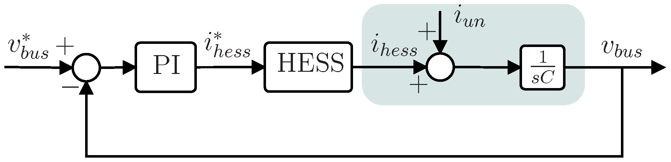
The structure of an FBM starts with the definition of a DC bus voltage loop. The objective of this loop is to keep the DC voltage constant and reject the disturbances caused by source and load variations. For this purpose, we first define the model of the bus as:
where is the voltage of the DC bus, C is the equivalent capacitance of the DC bus, is the total current of the HESS used to regulate the DC-bus voltage, and is a current that describes the power unbalanced between the RES and the load, i.e.,
where is the current provided by the RES and the current drawn by the load. It is worth noticing that the power of the unbalanced current can be viewed as a disturbance that needs to be compensated by the HESS.
In this case, since the HESS is composed of an SC and a BSS, we also have:
with and as the current of the SC and BSS, respectively.
If the power produced by the source equals the power demand of the load, then no action is required from the HESS (); on the contrary, if there is a power unbalance where the power demand is larger than the one produced by the RES, a positive action of the HESS will be needed () to maintain the balance; or if the generated power is greater than the drawn power, then there will be the possibility of storing energy in the HESS (). However, some conditions have to be taken into account: it is not recommended for the HESS to supply current when its level of storage energy is too low, or to draw current when the HESS is completely charged.
Figure 2 shows the simplified scheme of the voltage control for the FBM. This simple form has a bus voltage loop with a PI controller. It can be seen that the controller provides the reference current for the HESS, i.e., the current that is required from the HESS to keep the bus voltage constant, while the current is seen as a disturbance to be compensated.
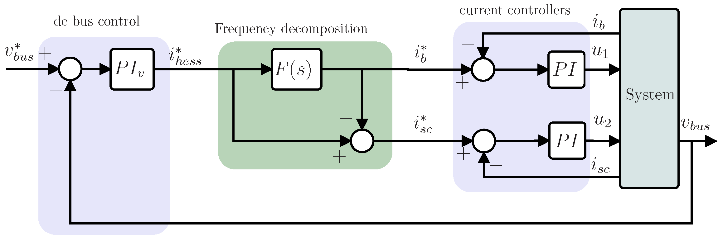
With reference to the total current of the HESS defined by the voltage loop, it is then necessary to split this power between the BSS and the SC. Figure 3 shows the EMS architecture for the conventional FBM. In this scheme, a low-pass filter decomposes the reference current in low- and high-frequency components, thus obtaining the current references for the BSS and the SC, and , respectively. In this way, it is obtained that:
and as a consequence
which keeps the invariance of the demanded current after the frequency separation.
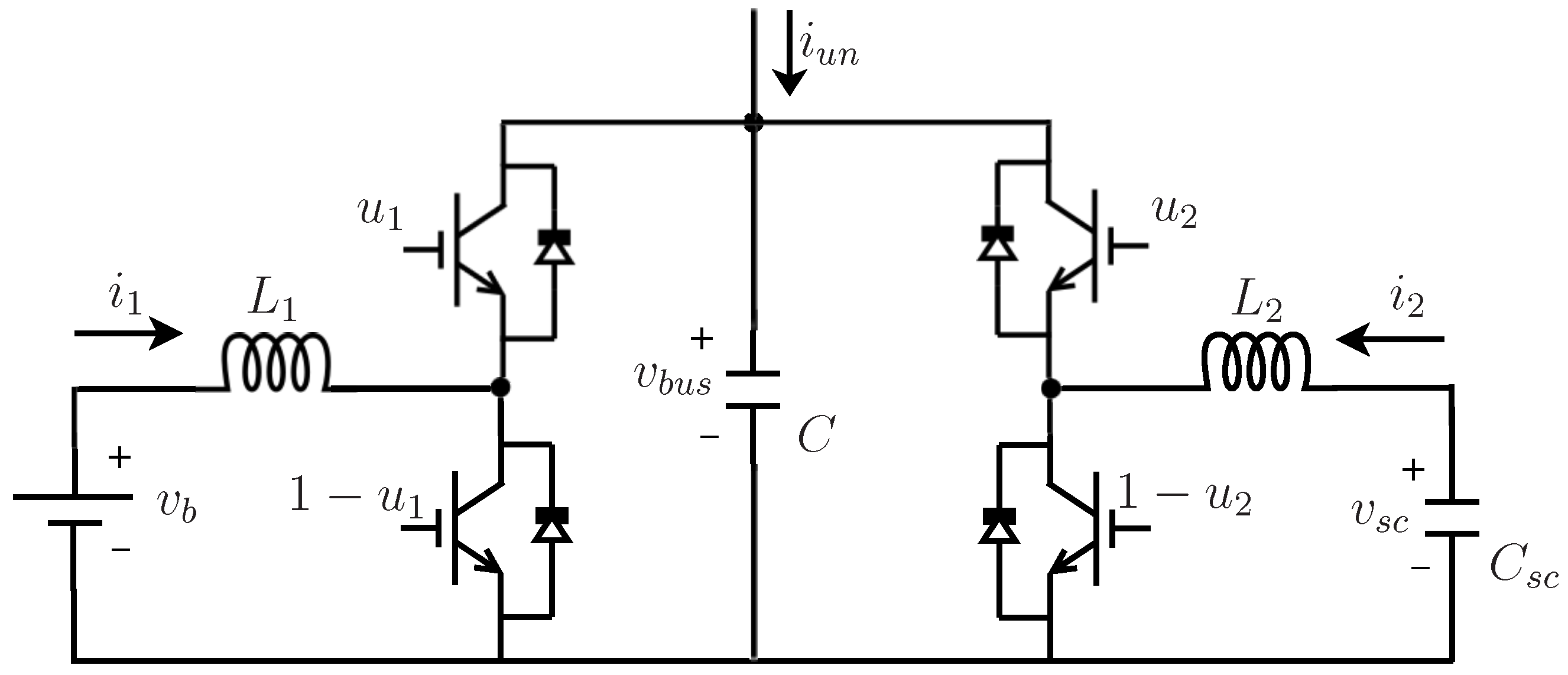
These two references, and , are then taken by the two current loops that control the power converters on each ESS. The current loops are commonly PI controllers, and the DC–DC converters are bi-directional power converters, as shown in Figure 4. Having these current loops involves that, only in a steady-state, the BSS and SC currents, and , will be equal to their corresponding references, and , respectively. Therefore, it is ideally expected that, in a steady-state:
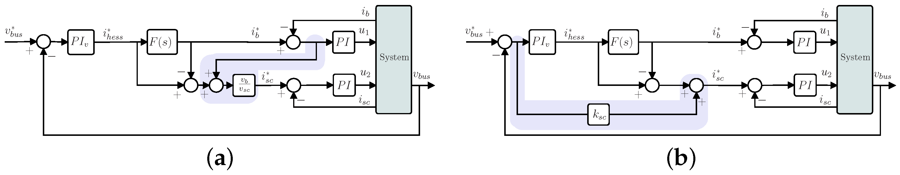
As can be inferred, during the transient state, Equation (7) does not hold, and as a consequence, the bus voltage regulation performance decreases. However, as the current loops are designed sufficiently faster than the outer voltage loop, it is expected that bus voltage variations caused by these transients are rapidly compensated. Furthermore, in order to improve this behavior, two modifications to the conventional structure can be found in the literature, which are also shown in Figure 5.
The proposals in [19,20,21,22,23] use a modification in which the error signal of the BSS current control loop is fed to the SC current loop with the aim of compensating for it using the fastest ESS (Figure 5a). In [24], the error of the voltage loop is fed to the SC current loop, thus using the SC to alleviate the transient response of the voltage loop controller (Figure 5b). All these structures help to improve the voltage regulation and reduce the stress in the BSS.
Under the conventional configuration, neither the voltage of the SC nor the SoC of the BSS is restored to predefined values. The parameters of the filter will establish the frequency separation of the power directly and the energy storage on each ESS indirectly. In this way, consider a first-order low-pass filter:
where is the design parameter that determines the cut-off frequency of the filter. A larger value of will lower the bandwidth of the filter and will make the SC provide more power, while the opposite occurs for smaller values.
Even though with the conventional FBM the frequency split of required power is performed, there are still more issues to rectify. In this manner, the EMS has to take into account the available energy in the storage device. This is an important aspect as to avoid premature degradation and extend the lifespan of the ESS, the SoC levels in both SC and BSS should be maintained within appropriate limits. What is more, keeping good levels in the SoC of the SC makes it available for the upcoming transients and load variations.
Three different approaches can be found to deal with the regulation of the SoC in FBM: bandwidth adjustment based on SC Soc, EMS rule-based strategies and SC SoC loop implementation. These strategies will be described below.
3.2. FBM with Adaptive LPF
The conventional FBM does not control the SoC in BSS or SC. However, SoC in each ESS can be indirectly adjusted by adapting the cut-off frequency of the LPF. A large bandwidth in the LPF will result in a lower use of the SC, whereas a low bandwidth does the opposite. As a consequence, the SoC of the ESS can be indirectly regulated using a time varying cut-off frequency in the LPF.
In [25,26,27], different strategies are proposed in which the bandwidth of the LPF is adjusted based on the SoC of the SC. It is shown how the energy level in the SC is kept within safe limits.
In [25], the topology of the HESS is semi-active; therefore, no control over the DC bus is performed. Although this strategy is thought to be used in electrical vehicles, this work is a good example of the regulation of the energy stored in the SC. The strategy adapts to the frequency of a first-order low-pass digital filter between a minimum and maximum value depending on the SoC of the SC. Consider the LPF in Equation (8) expressed as:
with as the cut-off frequency of the filter. The variation of proposed in [25] can be equivalently defined as:
with as the sampling frequency of the implemented digital filter and
where is the SC SoC and and are the maximum and minimum values of N to define minimum and maximum values for the cut-off frequency , respectively. The is, in turn, defined as:
with and as the maximum and minimum voltages allowed in the SC.
As an example, it can be interpreted from Equations (9) and (11) that if the load power is increasing, and the is at its minimum , then will be at its maximum, therefore lowering the use of the SC and its deep discharge. Similarly, if the load power is decreasing, and the is at its minimum , then N will be at its maximum and at its minimum, therefore increasing the use of the SC and allowing a faster charging process.
An index of impact on battery life is proposed based on the proposal in [28] and a comparison to fixed bandwidth filters is provided, showing that the adaptive strategy achieves lower battery degradation.
3.3. FBM with Rule-Based EMS
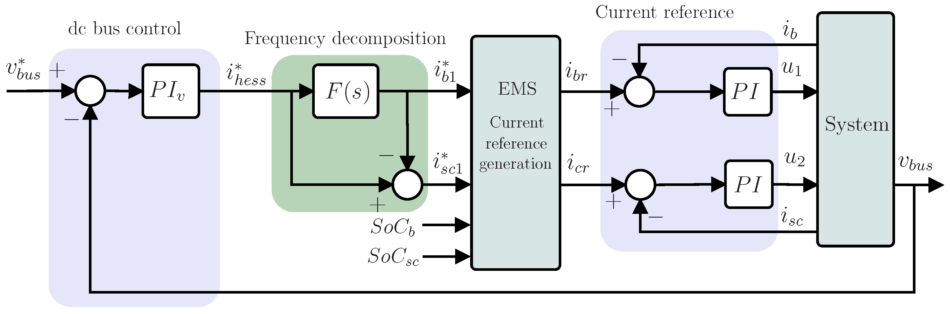
Within an FBM strategy, another approach to keeping the Soc of SC and/or BSS between safe limits is to use a rule-based EMS. In this case, the SoC of the ESS is monitored, and depending on its level and the energy available from the difference between sources and loads, a set of rules will determine the use of each storage device. Commonly, the rules will define the appropriate current references that will be sent to current controllers. A general structure of a rule-based EMS for the FBM is shown in Figure 6. It can be seen that the EMS receives the current references from the frequency decomposition part and with the information of the ESS, the SoC generates the final current references for each ESS. Two important modes are usually defined in a rule-based EMS: Power Excess (PE) means that the produced energy in the source is larger than the one demanded by the load, and power deficit (PD) means the opposite.
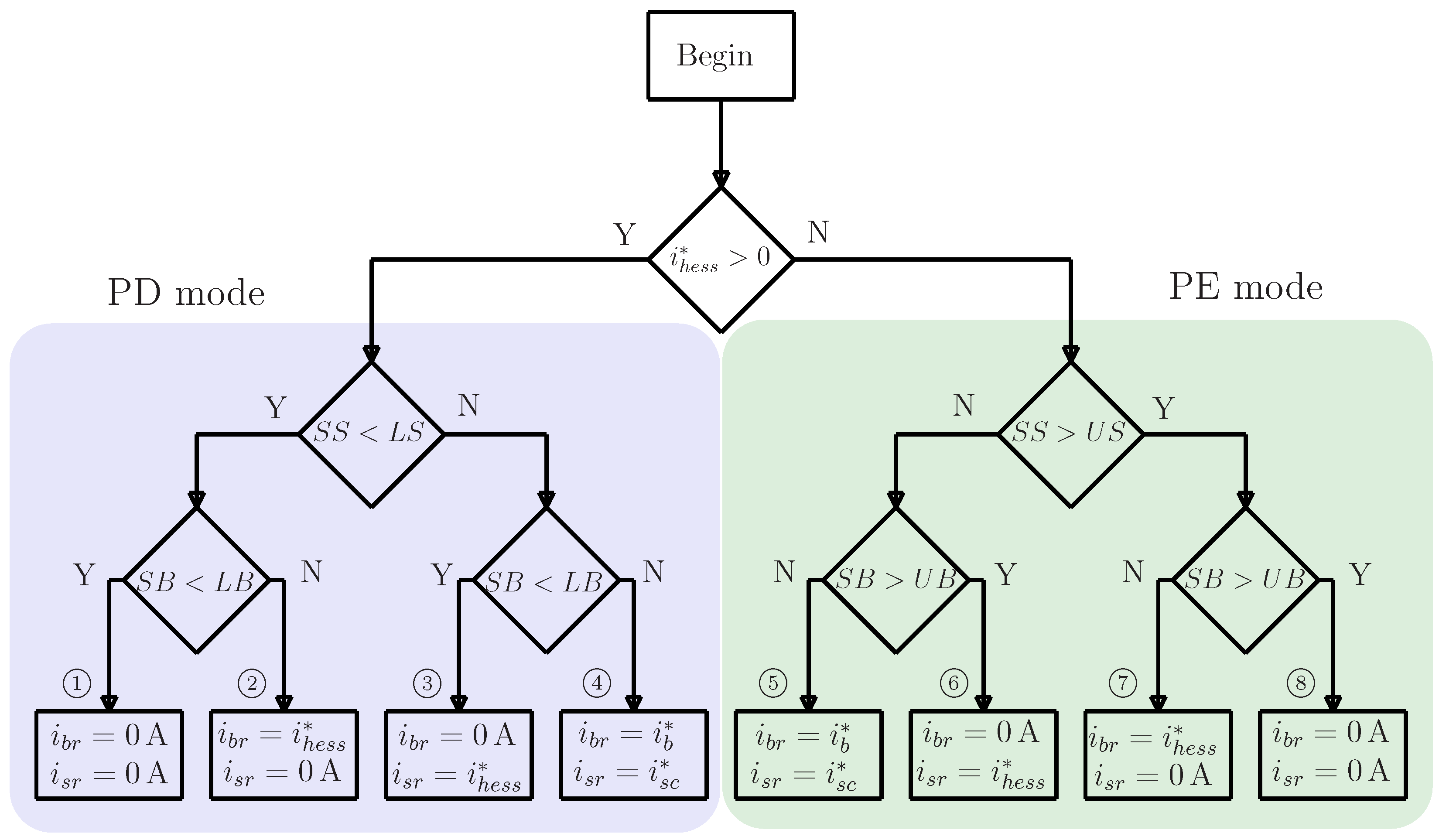
In [29], the effect the SC and filter parameters have over the battery rms current, energy efficiency, losses and current rate peaks is analyzed. A basic set of rules limits the use of the BSS and SC based on their SoCs. On power excess, if the SoC of the ESS is 95% or more, its reference current is set to zero as well as when, on power deficit, its SoC is lower than 25%. Figure 7 shows the complete flowchart of these rules. Simulation results show that even though there is no explicit regulation on the ESS SoCs, they are kept between the limits. Additionally, although not considered in the rules, an example is provided where the SC is charged by the BSS, which provides a constant current in predefined intervals of time. In this way, the SoC of the SC decreases slower while the BSS is discharged faster.
In [30], a rule-based EMS is proposed to maintain the SoC of the Bss and SC within predefined limits. In this strategy, PE and PD modes are defined in the top level of the rules, followed by conditionals regarding the SoC levels of the BSS and then the ones in the SC. The rules are similar to the previous work, where the current reference of the BSS is set to zero whenever its SoC is beyond the limits. However, the SC reference current is never set to zero. As the system includes a PV, there are rules to decide when to operate this source in Maximum Power Point Tracking (MPPT). In this manner, in PE mode, if the BSS has reached its SoC upper limit, then the MPPT mode is turned off and the PV will deliver the filtered demanded current . The simulation results show good bus DC regulation and the evolution of the SC and BSS SoC remained within limits. However, the behavior of the system has only been explored when the ESS is between the limits.
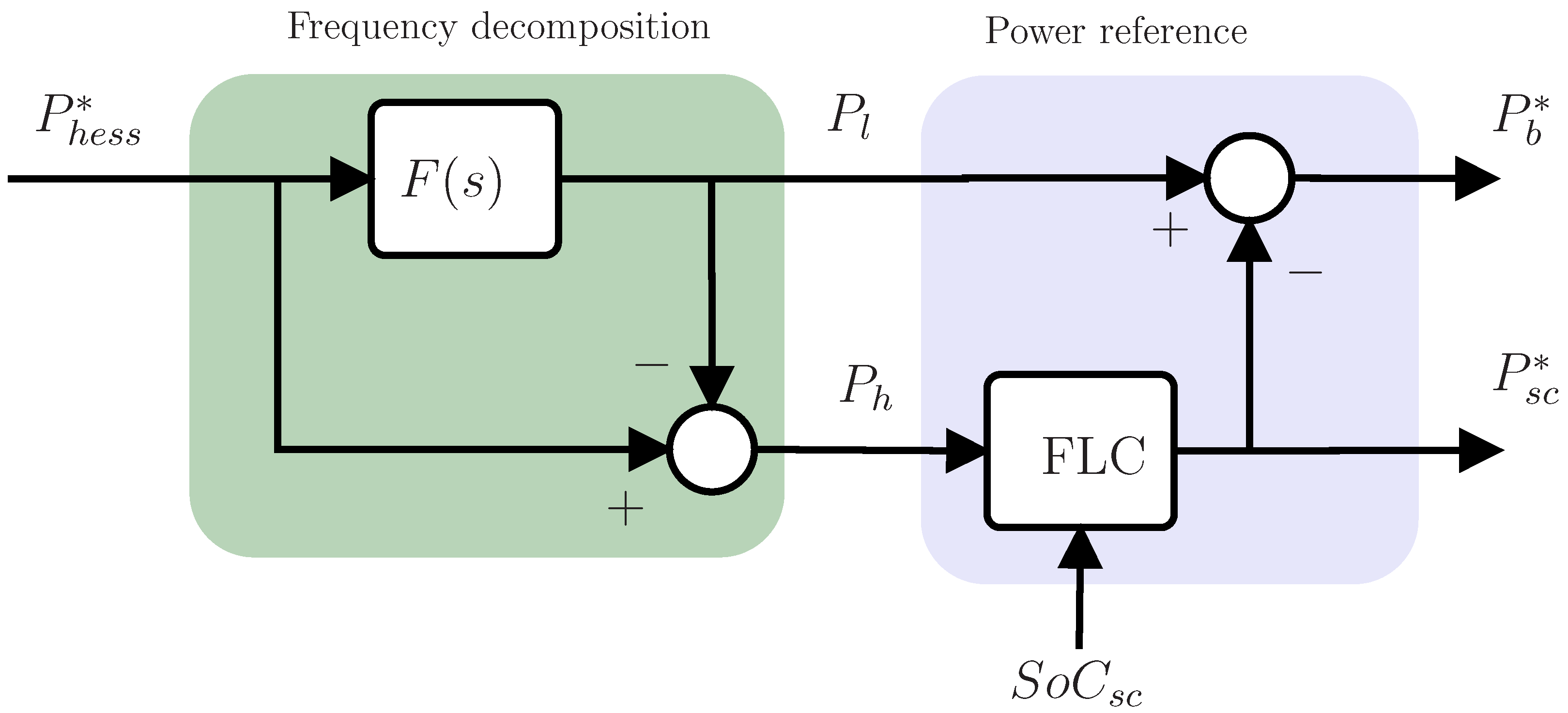
In [31], a semi-active topology with BSS and SC for EV is studied. The design of the LPF analyzes the impedance of the BSS and the DC–DC converter to set up its cut-off frequency. With the LPF, the high-frequency components of the demanded power are obtained, as shown in Figure 8. An FLC receives the , and with the information of the SoC of the SC, the corresponding power reference for the SC is determined . The FLC has three membership functions for the SoC: low, medium and high, and seven membership functions for the : high-negative, medium-negative, small-negative, zero, small-positive, medium-positive, and high-positive. The output of the FLC has seven membership functions that will define the power reference of the SC, which also consider charge and discharge modes: high-charge, medium-charge, slow-charge, zero, slow-discharge, medium-discharge, and high-discharge. Table 2 shows the rules of the FLC. For example, in the case of small-negative , the idea is to charge the SC, but if the SC is in high SoC the system will only apply a slow-charge to it. In this fashion, the SoC of the SC will remain in a safe interval. Finally, the BSS reference power is generated, subtracting the SC power reference to the demanded power , as shown in Figure 8, which makes the demanded power remain invariant.
Simulation and experimental results show that the SC SoC is kept within safe limits under the selected load profile. When compared to a basic EMS [32] and an offline optimization technique [33], it is shown that this strategy is closer to the optimal one in terms of the use of the BSS: rms, maximum, and squared value of the are used for comparison.
3.4. FBM with Rule-Based EMS and Sharing Coefficient
In addition to a rule-based EMS to limit the energy stored in the BSS and SC, the addition of a coefficient or function to gradually set the use of the ESS based on its SoC has been proposed in the literature. In this way, this coefficient or function is used to modify the current reference of the storage device, taking into account its SoC. As the rule-based EMS strategies described before only affect the ESS current reference when its SoC reaches upper or lower limits, an alternative is proposed, where a function or coefficient modifies this current reference gradually as the SoC approaches the limits. This action helps to improve the power allocation in the HESS.
Depending on the application, this approach has been used to regulate the use of the BSS or the SC.
3.4.1. Function for Power Allocation to Regulate SC SoC
Aimed at investment cost reduction, the work in [34] proposes an SC voltage regulation method based on a coefficient and the direction of the SC reference current. The structure of this controller can be seen in Figure 9. The parameter multiplies the SC command current and varies slowly from 1 to 0 as the SC voltage becomes close to its upper or lower limit. Additionally, some rules are disposed to take into account the charge and discharge mode of the SC, as shown in Table 3.
Therefore, according to Table 3, when the SC voltage is lower than a reference voltage and the SC reference current is positive, it indicates that the SC is required to deliver power and its voltage is going to decrease more; then, to avoid a large discharge, the coefficient will be used to reduce the current demand from the SC. The same applies when is larger than , and the command current is negative.
It will not be necessary to limit the current demand from the SC, i.e., , when the SC voltage is larger than a reference voltage and the SC reference current is positive, which indicates that the SC is required to deliver power and its voltage is going to decrease and become closer to the reference . The same applies when is lower than and the command current is negative.
It is worth noticing that if , then the BSS will be the only ESS in the HESS. Finally, simulation validation shows that the SC voltage remains around the reference voltage in V. Furthermore, it is shown that using a lower cut-off frequency in the LPF makes more often than using a higher bandwidth, and depending on the capacitance value, it might cause a larger use of the BSS.
3.4.2. Function for Power Allocation to Regulate BSS SoC
In addition to SC SoC, the BSS SoC can also be limited to stay within safe operational limits. Previously described strategies implement rules to produce this effect, obtaining a basic limiting functionally and once the BSS SoC reaches the limit, the corresponding charging or discharging current reference is set to zero. As described above for the SC SoC case, an alternative approach is to use a coefficient to gradually reduce the reference current as the BSS SoC approximates the limits. The difference in the case of the BSS is that this coefficient is used to share the power with an external source, such as RES (PV, FC, WT), or with the grid.
The work in [24] presents an application in a grid-connected HESS composed of a BSS and SC. In this case, the output of the low pass filter generates the averaged current , and this current is distributed between the BSS and the utility grid. The distribution is made based on:
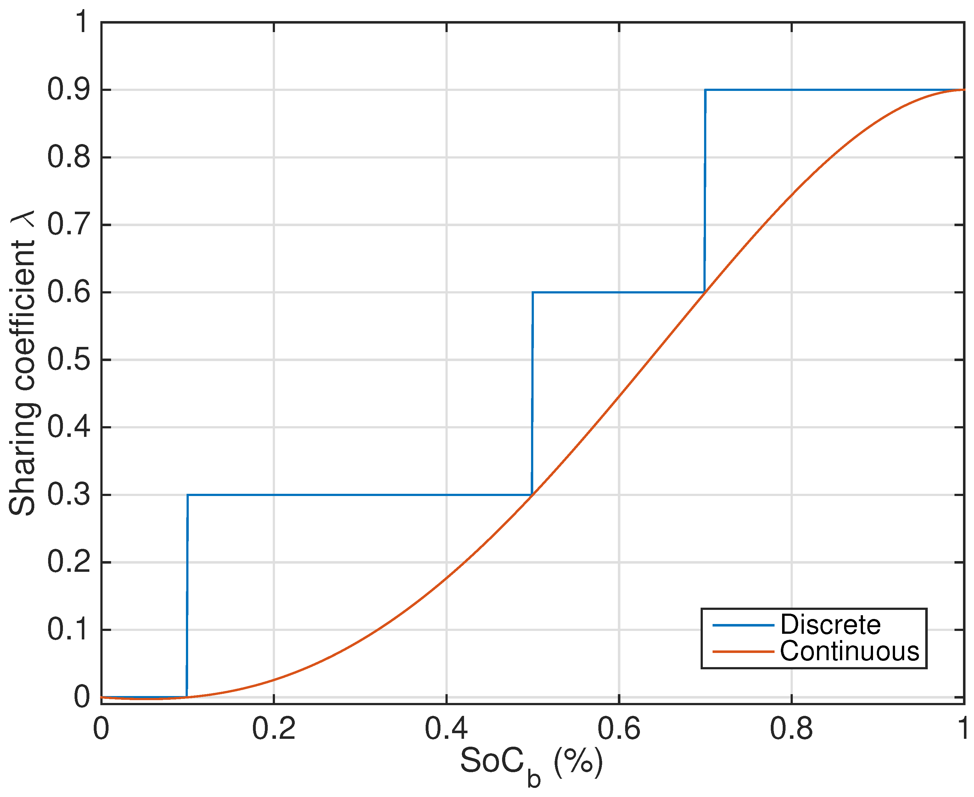
with the reference current of the BSS, the reference current of the grid, and the sharing coefficient. The value of is defined based on four levels of the BSS SoC, as shown in Table 4.
As a consequence, from Equations (13) and (14) and Table 4, if the BSS SoC is in its upper 70%, the BSS will deliver the total of the reference current , and the amount of current diminishes as the BSS SoC lowers until reaching the lower limit where the BSS current reference will be set as 0. It can be seen that the parameter is step-wise defined.
It is worth noticing that also the SC SoC is limited at its lower bound by setting its reference current to 0. To recover the BSS and SC SoC from the lower limit, it is proposed to charge the storage devices from the grid in the case of PD and from the RES in the case of PE. However, the evolution of the BSS and SC SoC is not studied in this proposal.
In a similar way, in [23], an EMS is proposed for a HESS with BSS and SC in the grid connected mode. On the one hand, when the BSS or SC reach the SoC limits, their reference currents are set to 0. On the other hand, if the BSS SoC is within safe limits, the averaged current reference is shared between the BSS and the utility grid. The sharing method follows Equations (13) and (14), and the most significant difference with the research in [24] is that this proposal uses a continuous defined coefficient instead of the discrete definition in Table 4. In this way, is defined as:
Figure 10 shows the comparative curve of the proposal [23,24]. It is shown that from Equation (15) is defined continuously with respect to the BSS SoC. The purpose of this definition is to avoid sudden changes in BSS current when its SoC reaches values that involve a discontinuous change in , in this way providing a smooth evolution for the whole interval.
The EMS is completed with the rules shown in Table 5. The conditions in this Table are equivalent to those in Figure 7, which is indicated through the added numbering. Comparing the rules in Figure 7 and in Table 5, it can be noticed how the addition of the grid provides more flexibility to the system and at the same time how more complex rules are created. Experimental results show that the rate of change in the BSS current, i.e., is lower with the new definition of in Equation (15).
3.5. FBM with SoC Restoration Loops
Large fluctuations in the SC SoC can cause the SC operational safe limits to be exceeded, which is why a continuous regulation of its SoC is considered advantageous.
In order to provide this functionality, an SoC feedback loop has to be added to the control structure, which will generate an additional current (or power) reference. The way these references are generated and added to the existing EMS is the difference between the approaches in the literature.
In the previously described proposals, the SoC of the ESS is limited within safe limits, and some rule-based strategies include a charging procedure in the case that the ESS SoC has reached the lower limit. The proposal in [34] described in Section 3.4.1 is similar to a closed-loop technique since it adds a reference SC voltage and takes actions based on measured values of this voltage . However, the strategy uses a rule-based decision method together with a weighting coefficient to set the reference current of the SC.
In the following, different SC voltage restorage strategies will be discussed.The work in [35], presents an EMS for a standalone MG that is constituted by the HESS and two renewable sources: a PV panel and a PEM FC. A Moving Average Filter (MAF) is used to separate high- and low-frequency current components. The MAF is also used in proposals such as [36,37]. MAF usually have a good time response but poor frequency response compared to LPF [38].
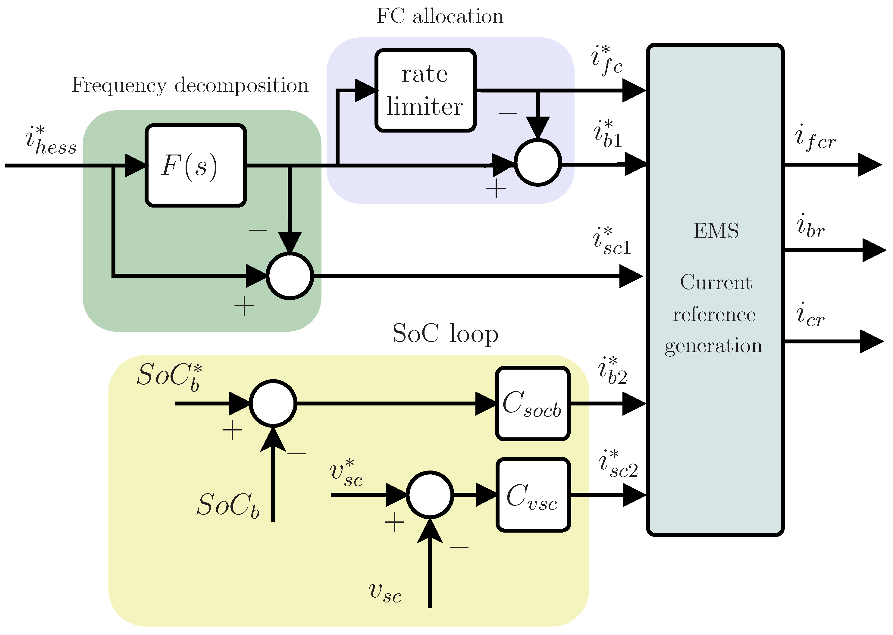
Figure 11 shows the structure proposed in [35]. The average current is distributed between the BSS and the FC, where a rate limiter separates the current that is required for the FC, and the remaining current will be provided by the BSS.
The EMS defines PE and PD modes. Similarly to rule-based strategies, while in the PE state, if the SoC of the SC and BSS are in the upper limit, their current references are set to 0; and in PD mode, the current references of the SC and BSS are set to 0 if their corresponding SoC lower limits are reached. The main difference comes from the addition of SoC control loops for SC and BSS. However, these loops only take action when the system is in PE mode and the SoC of the SC and BSS are at their lower bound. This means that the SC and BSS will be charged using the excess power through the SoC control loops. For other different conditions, these loops are disabled.
The current reference from the SoC loops is generated by (see Figure 11):
where and are the controller transfer functions of the SC and BSS SoC, respectively, which are proposed to be PI compensators. Thus, In PE mode, when the SC and BSS reach their SoC lower limits, references and are added to the ones generated after the low pass filter, thus having:
The complete set of rules is defined in Table 6. It can be observed that the rule described by Equations (18) and (19) is new with respect to other proposals, and the rules for conditions (1) to (8) are somehow similar to other approaches with the difference of having an FC as a secondary source in this case. Simulations and experimental results show scenarios where the SoC of SC and BSS reach the upper limit, although no evidence of the evolution of the system under the charging loop operation is portrayed.
An interesting method to calculate the power separation filter parameters, the SC SoC control loop, as well as the size of the SC is presented in [39]. This work presents a HESS that, although based on an AC bus, proposes an SC Soc loop that continuously regulates the energy in the SC. In this case, the SoC loop is based on the SC energy instead of SC voltage. The authors claim that employing an energy loop avoids the nonlinearities that appear when using a voltage loop controller, thus making the calculation of the HESS parameters and sizing of the SC easier. Works that make use of an SC voltage loop can be found in [17,40,41,42,43].
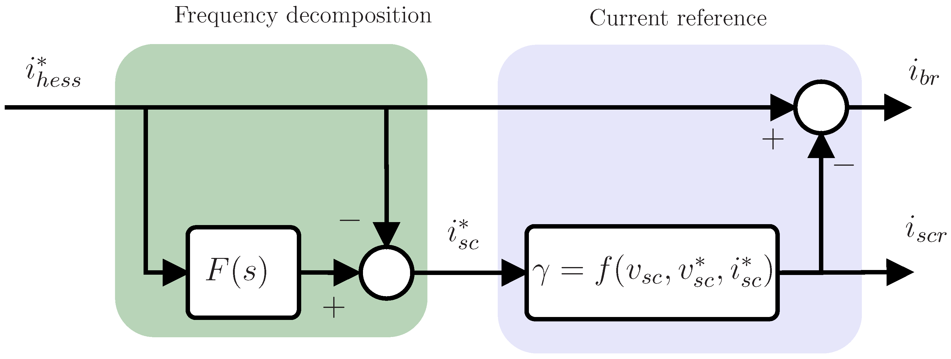
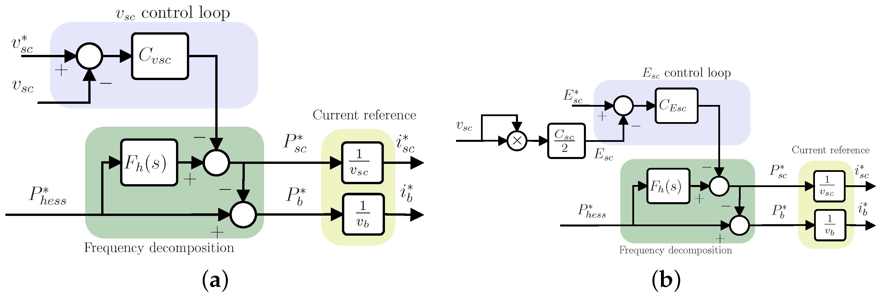
Instead of using an LPF for frequency component separation, a High Pass Filter (HPF) is used. In this way, the output of the HPF will select the high-frequency components to set the current reference of the SC. Figure 12 shows the SC voltage loop in [41] and the energy loop in [39] proposed by the same authors.
It can be observed that both approaches have the same structure; however, the signals used in the SoC regulation are the SC voltage in [41] and the SC energy in [39].
For the energy loop approach, it can be observed that the output of the energy loop controller is added to the output of the HPF to obtain the SC power reference. Finally, this power is divided by the SC voltage to obtain its current reference:
where is the transfer function of the HPF, is the total power demanded to the HESS, is the energy loop controller proposed to be a constant gain, is the SC energy reference, and is the energy in the SC, which can be calculated as:
Alternatively, the reference current for the BSS results is:
The strategy is validated experimentally, showing that the SC voltage remains within safe limits.
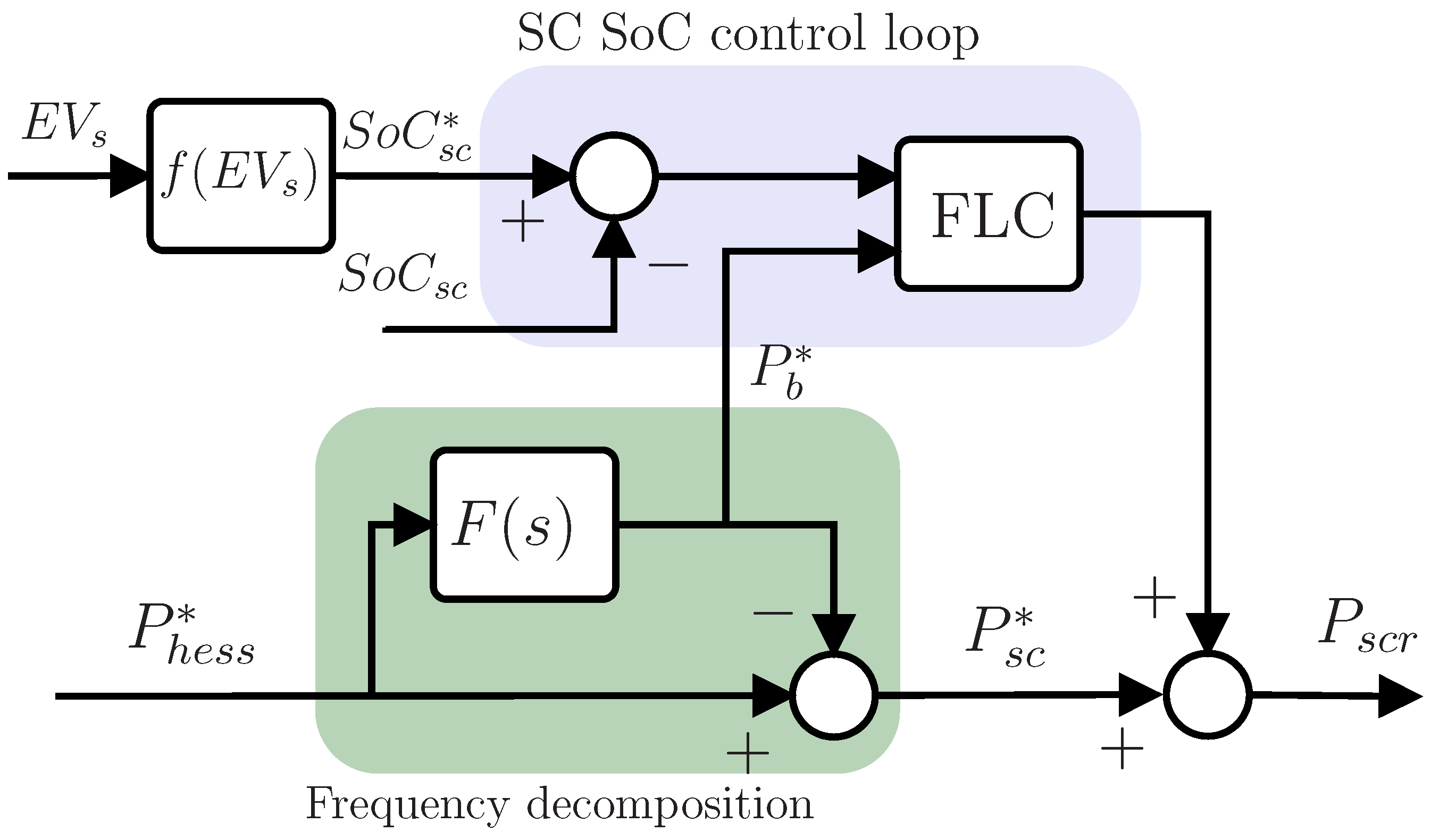
The proposal in [44] is a semi-active HESS topology for EV where the BSS sets the DC bus voltage and the SC is connected to it through a DC–DC converter. In this approach, the LPF is the base for generating the current reference for the SC as is achieved in the conventional FBM.
An SC SoC loop is proposed where the reference SoC is variable; in this case, it is defined using the velocity of the EV, . This is an interesting idea since this varying setpoint can be used to provide more flexibility to the HESS.
Figure 13 shows the block diagram for this proposal. As it can be seen, the SC SoC reference is compared with the measured one , and the error is processed by an FLC, which also receives the power reference for the BSS and generates a signal that is then added to the SC power reference from the LPF stage.
The FLC has three membership functions for the SoC error : negative, medium and positive, and five membership functions for the BSS power reference : high-negative, small-negative, medium, small-positive, and high-positive. The output of the FLC has four membership functions that will define the power to be added to the reference of the SC obtained form the LPF: high-charge, medium-charge, slow-charge, zero, slow-discharge, medium-discharge, and high-discharge. Table 7 shows the rules of the FLC. Experimental results show that the SC fulfills the requirement of providing high-frequency current components. Although the SoC reference signal is not provided, it can be observed that the SC voltage is kept within allowable variations.
4. Numerical Analysis
In this section, four of the most relevant reported improvements to the FBM performance were selected to be compared and analyzed. In this way, it was considered that rule-based EMS, the power sharing coefficient, and the SoC loop implementation are interesting strategies that contribute to the development of HESS.
It is found that for the rule-based EMS, the set of conditions and rules are similar, some differences appear as external sources are added, and the work in [29] is selected as an example of this. In the case of the power sharing coefficient, the proposal presented in [34] has the advantage of combining a small set of rules with the sharing coefficient to keep the SC voltage within the limits. Finally, in the case of SoC regulation using control loops, it is interesting how in the approach in [35], the SC SoC loop can take the place of a rule-based EMS to preserve the functionality of the SC.
4.1. Simulation Setup
The performance of the HESS based on the four above-mentioned approaches was compared and analyzed through simulation.
Although the selected proposals are not fully reproduced here, the most relevant characteristics for the purpose of this paper were taken into consideration. Additionally, for comparison purposes, the parameters of the filter, controllers, and circuit elements were adjusted and unified. All parameters and values can be found in Table 8. It is important to note that the simulation results and analysis presented here are not included in the original articles.
The following structures are simulated:
The frequency decomposition filter for CON, RB and COEFF is defined as the first-order LPF in (8) while, for equivalence, the HPF filter for COEFF is defined as:
with s, as shown in Table 8.
The simulation was performed in Matlab, Simulink, and the averaged model of the power electronics was used. The evolution of the HESS was investigated mostly in PD mode since the PE mode yields similar results.
4.2. Simulation Results
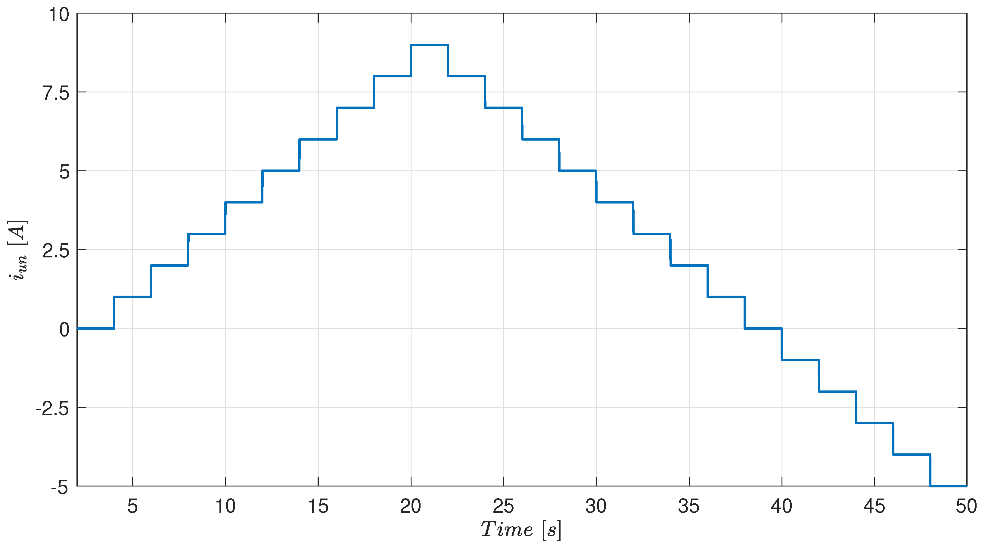
The unbalance between the source and the load is depicted through the current (as in Equation (2)) in Figure 15. This current profile is defined to evaluate the behavior of the HESS when the SC SoC reach the lower limit and to observe the transition from PD to PE modes, which occurs at s.
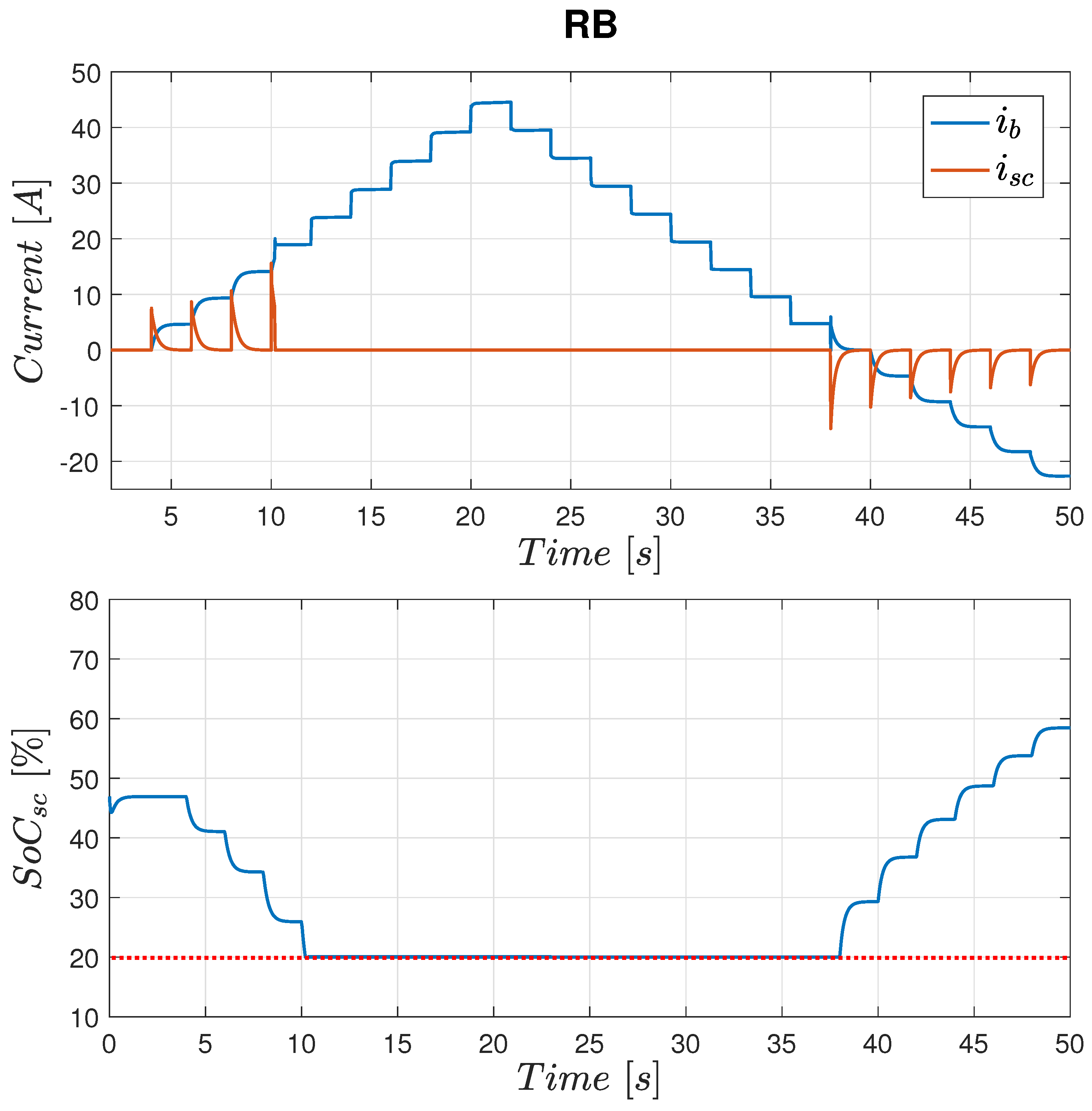
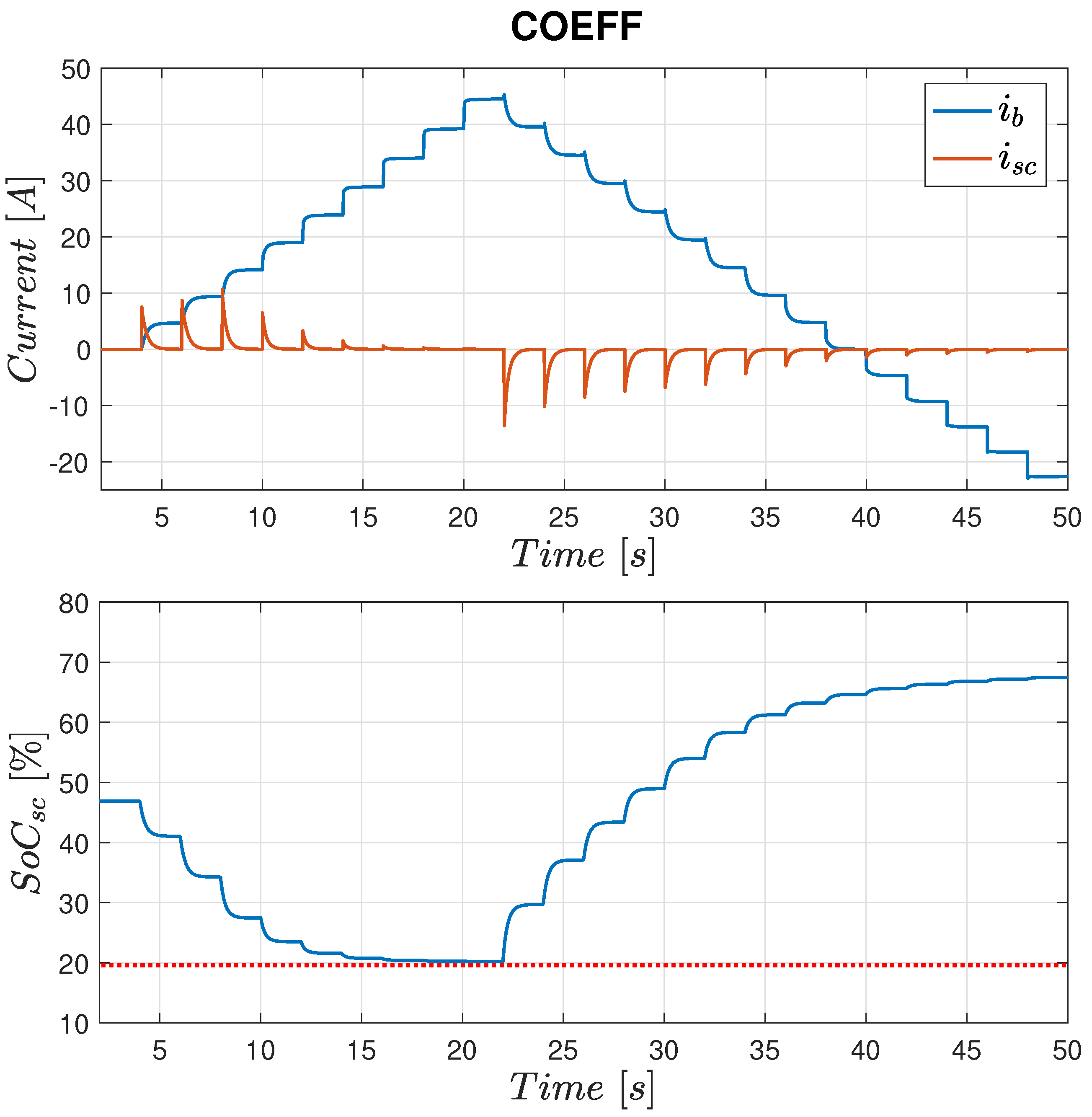
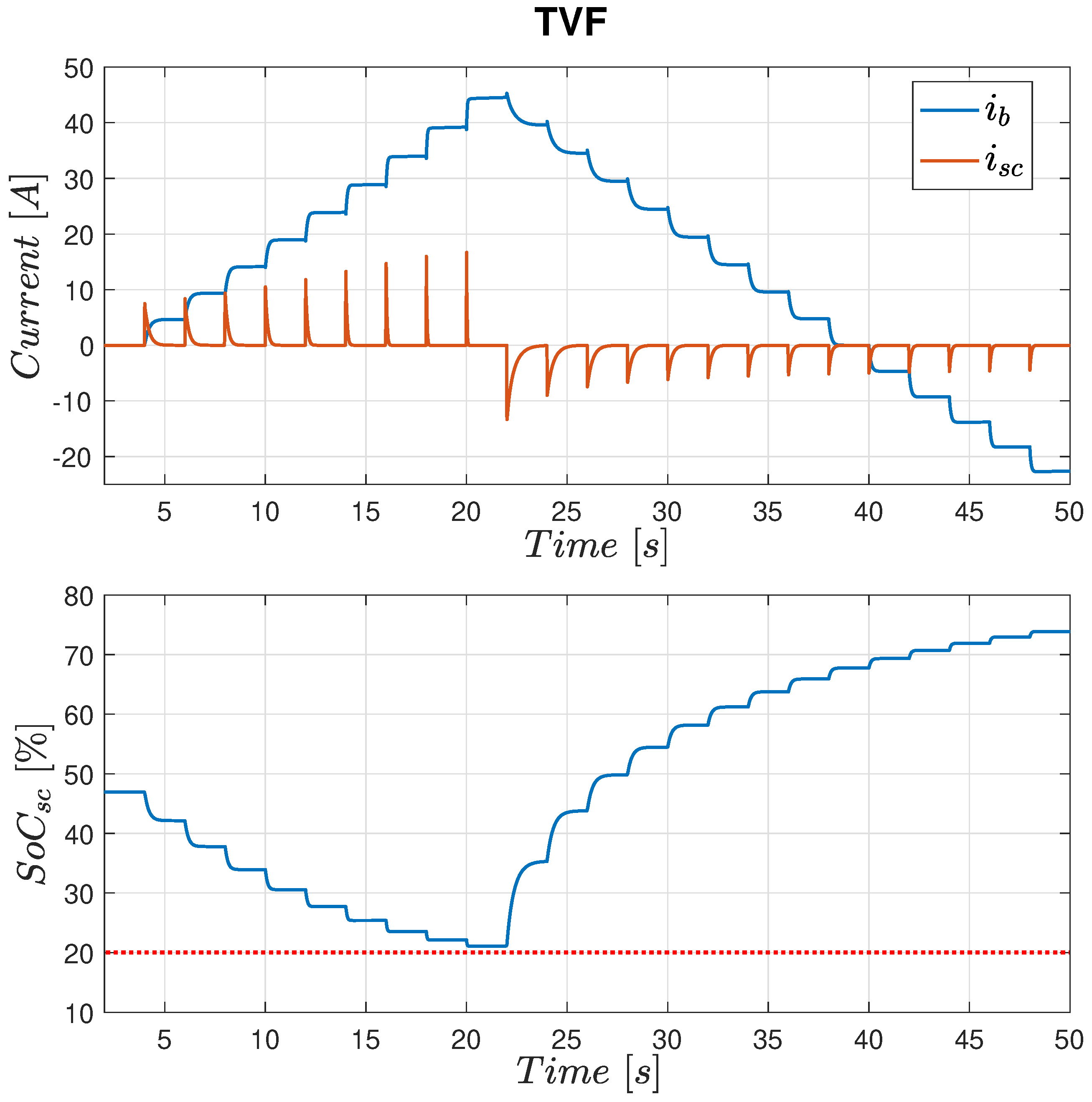
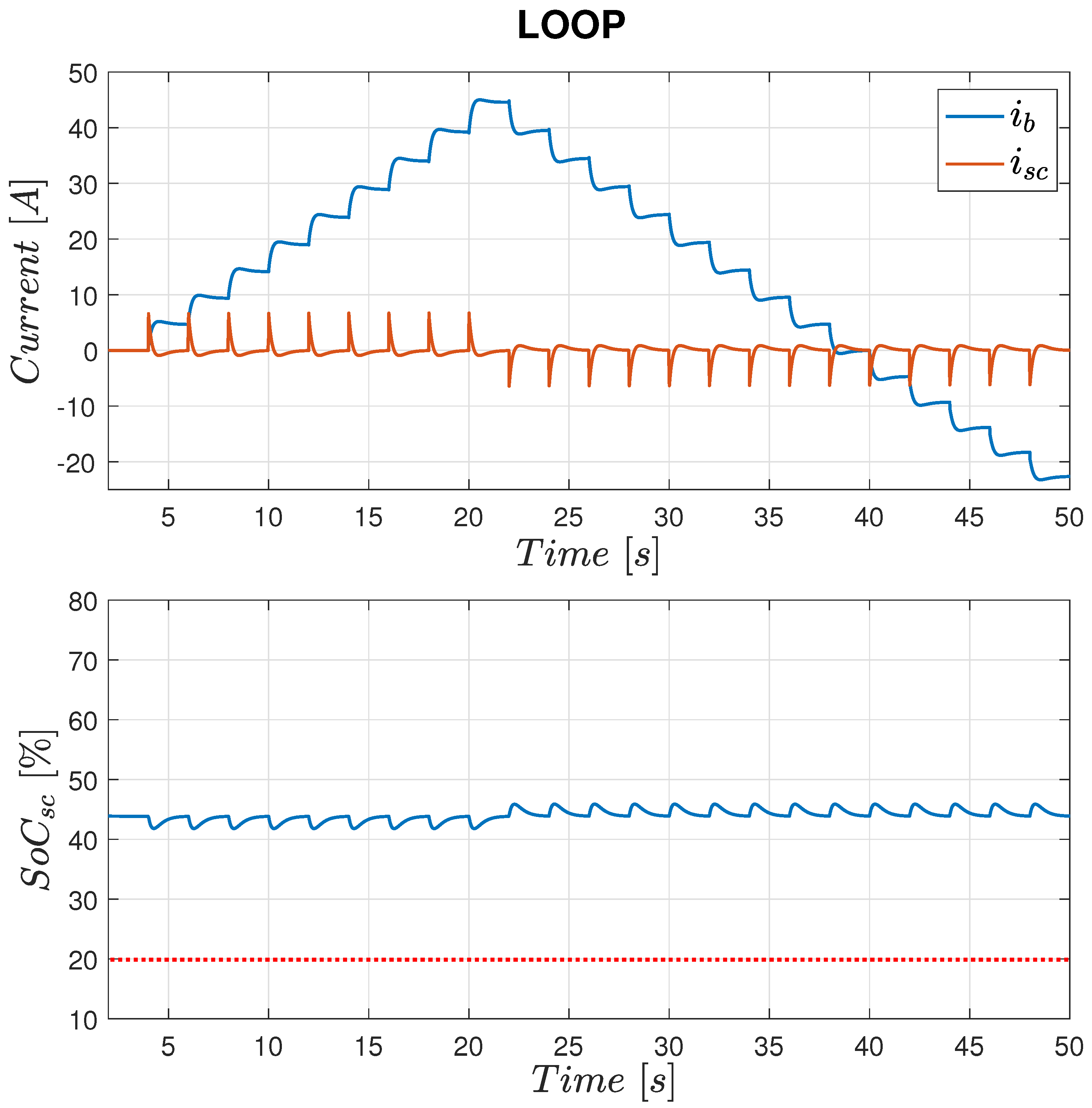
Figure 16, Figure 17, Figure 18 and Figure 19 show the evolution of the SC and BSS currents and SC SoC under the unbalanced current in the RB, COEFF, TVF, and LOOP cases, respectively. In all cases, it can be seen that when the SC has enough stored energy, it successfully takes the fast current variations while the BSS is in charge of the slower current components. Additionally, the SC and BSS keep their operation within safe operational SoC limits.
In addition, the following can be observed:
- RB case: As shown in Figure 16, from the starting time s to the second s, the HESS works under the conditions for rule 4 shown in Figure 7; therefore, the SC is delivering the high-frequency current components and the BSS provides the lower ones. Then, the current of the SC is set to 0 A when the SC SoC reaches the lower limit 20% (conditions for rule 2). At that moment, the BSS current starts to have a sharper profile since it is the only ESS left. During this period, degradation of the BSS is caused. When the current makes the transition to the PE mode (at ), the SC is able to receive the current from the FBM control system and increases its SoC (conditions for rule 5). In total, the HESS operates without the SC for the period of time its SoC is at the lower limit, causing some degradation in the BSS.
- COEFF case: From the initial time, it can be seen that the current in the SC is providing the fast current components of the HESS. Then, as the SC SoC decreases, the amplitude of the current is made lower due to the action of the sharing coefficient . This also affects the current of the BSS, which becomes sharper. In comparison with the RB case, although both systems cause degradation on the BSS, in the COEFF case, the SC reduces its operation in a smoother way, which makes it work for longer. For that reason, a lower degradation in the BSS is expected. However, it can also be seen that the SC reaches the SoC upper limit since it receives energy even before the PE mode transition. This means that large SoC excursions are not avoided under this strategy.
- TVF case: Figure 18 shows the results for this case. Since the cut-off frequency depends on the SC SoC, it is seen that as the SoC decreases and increases, a lower usage of the SC is obtained. As a consequence, from time s to s, the current signal provided by the SC becomes narrower. After s, when current begins decreasing, the process starts over but, in this case, with the SC SoC rising up. Thus, Equation (12) creates a soft transition in the SC utilization, which, with the selected setup, reduces/increases the SC SoC in a slower way compared to the COEFF case. An additional difference is that, since there is a lower limit for , the SC always responds against sudden changes in , which reduces the BSS degradation when the SC is close to the SOC limits. As with the previous strategies, large SoC excursions are not avoided.
- LOOP case: Resulting HESS currents and SC SoC for this case are shown in Figure 19. It can be observed that the SC is always contributing to the high-frequency current components with the same dynamic response. Thus, for the whole time interval, the SC absorbs/delivers power when fast current changes appear, which avoids the BSS degradation. The SC SoC response shows the effect of the added SoC loop. In this way, after every fast reaction of the SC, the SoC loop regulates the SC voltage to the desired level ( V). As a result, this strategy achieves a flatter response that avoids large variations in the SC SoC and voltage. It is worth noticing that this SoC regulation implies a larger, although smooth, use of the BSS, which delivers the energy to make the SC SoC control possible.
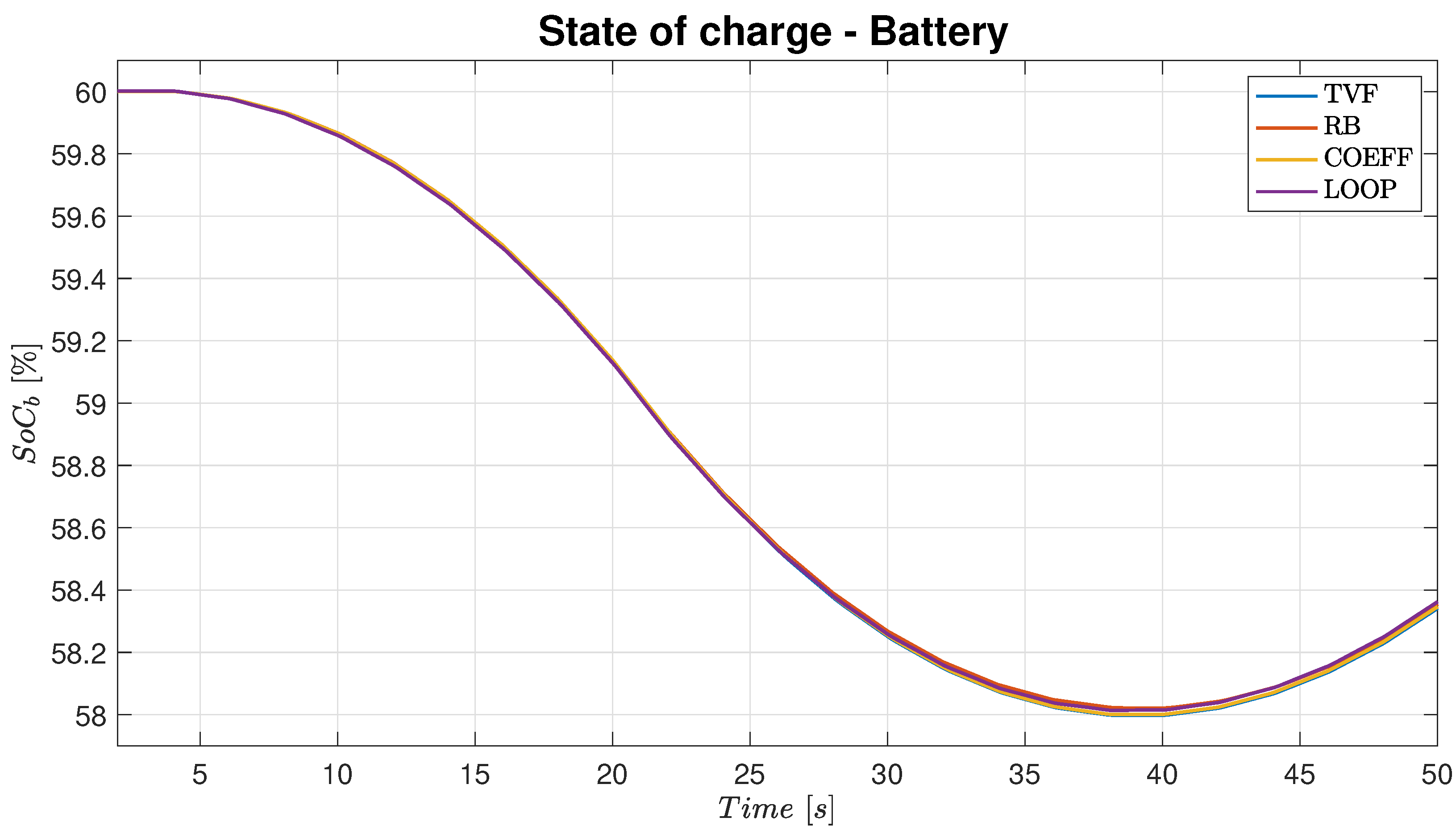
Figure 20 shows the evolution of the BSS SoC under the unbalanced current shown in Figure 15. It is observed that for all cases, the SoC evolution in the BSS is practically the same. The PD and PE modes are evident as after s the BSS SoC changes its decreasing trend to an increasing one.
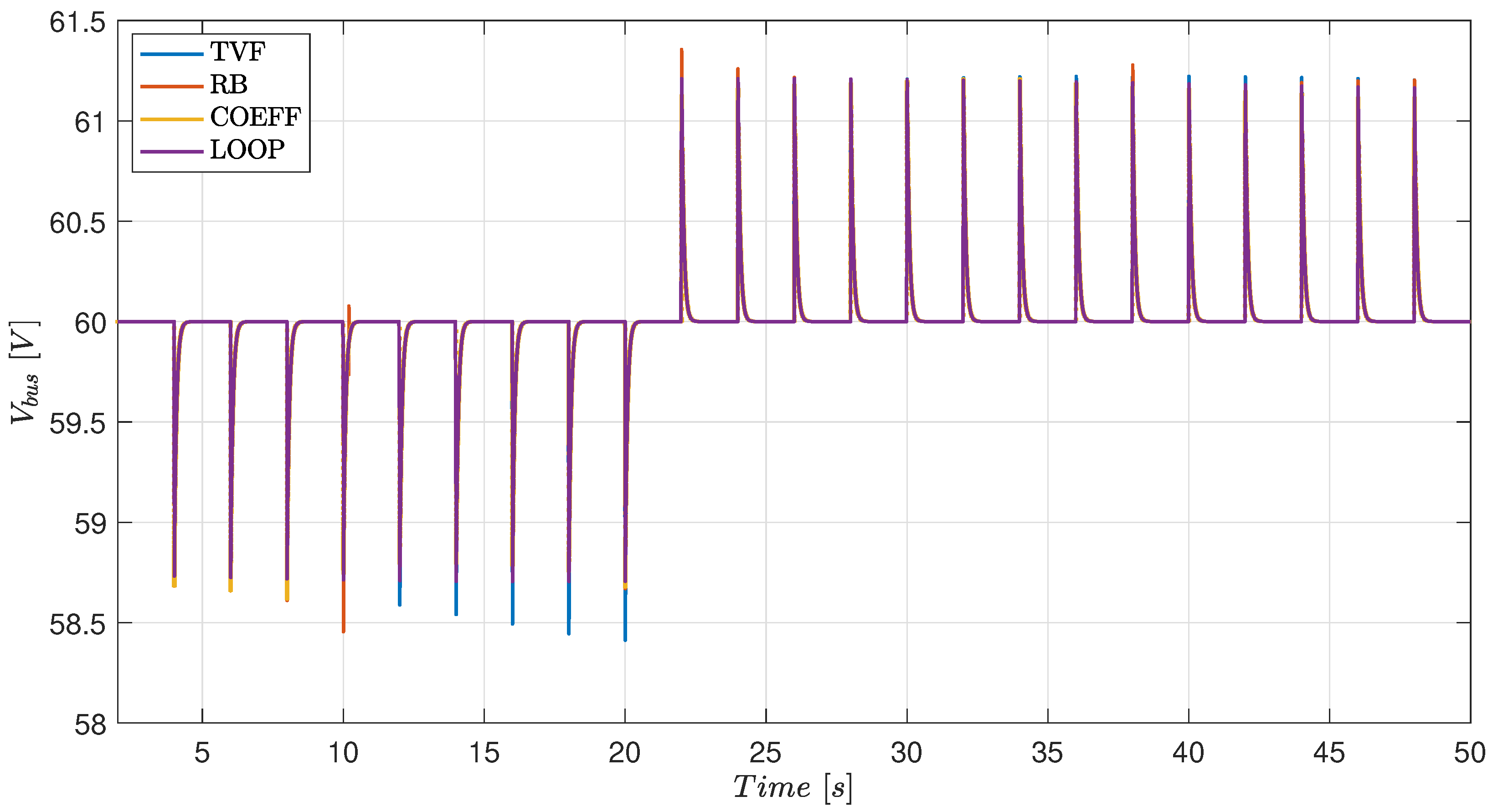
This voltage behaves in a very similar manner for all the cases, keeping its steady-state value at the reference voltage V.
In Figure 21, the DC bus voltage is depicted.
Table 9 summarizes the general advantages and disadvantages of the analyzed methods.
5. Final Discussion and Conclusions
The FBM exhibits one of the most simple architectures in which an EMS can be based to create a successful integration of HESS. The last published research works analyzed in this paper show the evolution of this technique, which has been adapted from its conventional form with the objective of providing more functionalities and flexibility.
In this manner, an EMS has been incorporated in the form of rules, FLCs, sharing coefficients, and complemented with additional control loops.
Improvements to the FBM seek to avoid the premature degradation of the ESS. When working with BSS, degradation comes from deep discharge, overcharge, and fast current variations, while overcharge is the main concern in the SC. Since the FBM mitigates fast currents in the BSS, the enhancements are then focused on keeping the BSS and SC working within safe operational limits.
Proposals based on rules started with the basic form of the work in [29], which is shown in Figure 7. With these rules, once the ESS reach an SoC limit, its current is set to 0. This means that, in order to keep the bus voltage, if one of the ESSs is with i = 0 A, then the remaining ESS will supply the total demanded current. Thus, it is possible that in some cases, the BSS works by delivering peaks of current, which decreases its lifespan. Additionally, in the rules in Figure 7, there is no method to recover the SoC in the HESS. The proposals in [23,35] add this functionality, in this way providing methods to charge SC or BSS when there is energy available from an external energy source (RES, FC or grid). The charging process is usually performed at a constant current using the rated charge current of the devices.
Extending the operation of the HESS to its maximum is one possible improvement at this point. In the methods in [23,24,34], the SC and BSS can also reach the SoC limits, but this is achieved gradually, in this way extending the operation of the ESS. To achieve that, a sharing coefficient is added, which will take effect when the SoC of the ESS approximates the limits. The SC will gradually reach the limit, sharing the power with the BSS [34], while the BSS will share the power with an external source [24]. The advantage of the method in [24] is that it provides a way to extend the operation of the HESS based on the available external energy. While in [34], the SC operation can be extended thanks to the BSS, which will extend the protection of the BSS from delivering/absorbing large current peaks. The approach in [23] improves the one in [24], defining a continuous varying coefficient instead of a discrete one, which avoids sudden changes in the BSS current.
From previous proposals, it is expected that better regulation of the ESS SoC would bring more benefits. That is how the proposal in [35] adds SoC loops for BSS and SC; however, these loops are only used when the devices reach the lower limit of the SoC, and they are disabled otherwise.
In [39], the goal is to keep the voltage of the SC at a given value through a voltage/energy loop. The main advantage is that this loop is active all the time, which produces an automatic and continuous regulation of the SC voltage. Furthermore, this will further extend the operation of the SC, which in turn will extend the BSS life cycle.
Finally, the work in [44] proposes a varying SoC reference; in this case, it depends on the EV speed. The advantage of the constant SoC reference has not been exposed; however, the idea can provide more flexibility to the HESS.
In conclusion, it can be observed that more research is needed to investigate the evolution and behavior of the SoC with the aim of extending the operation of the HESS as much as possible while also avoiding the premature degradation of each ESS. As future work, it might be necessary to explore in-depth the advantages that those approaches that continuously regulate the SoC of the ESS can bring. For example, approaches that continuously regulate both the SoC of the SC and the BSS with the addition of RES and/or the utility grid.
Finally, and in the same direction as SoC regulation, the benefits of having variable SoC references need to be explored. For example, the definition of optimal SoC references could be an interesting topic to discuss.
Author Contributions
Conceptualization, G.A.R.; writing—original draft preparation, G.A.R.; writing—review and editing, R.C.-C.; supervision, R.C.-C. All authors have read and agreed to the published version of the manuscript.
Funding
This research is part of the CSIC program for the Spanish Recovery, Transformation and Resilience Plan funded by the Recovery and Resilience Facility of the European Union, established by the Regulation (EU) 2020/2094, CSIC Interdisciplinary Thematic Platform (PTI+) Transición Energética Sostenible+ (PTI-TRANSENER+) and the Spanish Ministry of Economy and Competitiveness under Project DOVELAR (ref. RTI2018-096001-B-C32).
Institutional Review Board Statement
Not applicable.
Informed Consent Statement
Not applicable.
Data Availability Statement
Not applicable.
Conflicts of Interest
The authors declare no conflict of interest.
Abbreviations
The following abbreviations are used in this manuscript:
| BSS | Battery Storage System |
| DC | Direct Current |
| DGS | Distributed Generation System |
| EMS | Energy Management System |
| ESS | Energy Storage System |
| FBM | Filter-Based Method |
| FLC | Fuzzy Logic Control |
| HEDS | High Energy Density Storage |
| HESS | Hybrid Energy Storage System |
| HPDS | High Power Density Storage |
| HR | Heuristic Rules |
| MAF | Moving Average Filter |
| MG | Microgrids |
| MPPT | Maximum Power Point Tracking |
| PE | Power Excess |
| PD | Power Deficit |
| RES | Renewable Energy Source |
| SC | Supercapacitors |
| SoC | State of Charge |
| UnC | Underlying Control |
References
- Nair, U.R.; Costa -Castelló, R. An overview of micro-grid architecture with hybrid storage elements and its control. In Proceedings of the XV Simposio CEA de Ingeniería de Control, Salamanca, Spain, 9–10 February 2017. [Google Scholar]
- Nair, U.R.; Costa-Castelló, R. A Model Predictive Control-Based Energy Management Scheme for Hybrid Storage System in Islanded Microgrids. IEEE Access 2020, 8, 97809–97822. [Google Scholar] [CrossRef]
- Li, X.; Hui, D.; Lai, X.; Yan, T. Power Quality Control in Wind/Fuel Cell/Battery/Hydrogen Electrolyzer Hybrid Micro-grid Power System. In Applications and Experiences of Quality Control; Ivanov, O., Ed.; IntechOpen: Rijeka, Croatia, 2011; Chapter 29. [Google Scholar] [CrossRef] [Green Version]
- Shayeghi, H.; Shahryari, E.; Moradzadeh, M.; Siano, P. A Survey on Microgrid Energy Management Considering Flexible Energy Sources. Energies 2019, 12, 2156. [Google Scholar] [CrossRef] [Green Version]
- Etxeberria, A.; Vechiu, I.; Camblong, H.; Vinassa, J.M. Comparison of three topologies and controls of a hybrid energy storage system for microgrids. Energy Convers. Manag. 2012, 54, 113–121. [Google Scholar] [CrossRef]
- DiCampli, J.; Laing, D. State of the Art Hybrid Solutions for Energy Storage and Grid Firming. In Proceedings of the POWER-GEN & Renewable Energy World Europe, GE Power, Cologne, Germany, 27–29 June 2017. [Google Scholar]
- Khaligh, A.; Li, Z. Battery, Ultracapacitor, Fuel Cell, and Hybrid Energy Storage Systems for Electric, Hybrid Electric, Fuel Cell, and Plug-In Hybrid Electric Vehicles: State of the Art. IEEE Trans. Veh. Technol. 2010, 59, 2806–2814. [Google Scholar] [CrossRef]
- Dong, C.; Jia, H.; Xu, Q.; Xiao, J.; Xu, Y.; Tu, P.; Lin, P.; Li, X.; Wang, P. Time-Delay Stability Analysis for Hybrid Energy Storage System With Hierarchical Control in DC Microgrids. IEEE Trans. Smart Grid 2018, 9, 6633–6645. [Google Scholar] [CrossRef]
- Hajiaghasi, S.; Salemnia, A.; Hamzeh, M. Hybrid energy storage system for microgrids applications: A review. J. Energy Storage 2019, 21, 543–570. [Google Scholar] [CrossRef]
- Sikkabut, S.; Mungporn, P.; Ekkaravarodome, C.; Bizon, N.; Tricoli, P.; Nahid-Mobarakeh, B.; Pierfederici, S.; Davat, B.; Thounthong, P. Control of High-Energy High-Power Densities Storage Devices by Li-ion Battery and Supercapacitor for Fuel Cell/Photovoltaic Hybrid Power Plant for Autonomous System Applications. IEEE Trans. Ind. Appl. 2016, 52, 4395–4407. [Google Scholar] [CrossRef] [Green Version]
- Faisal, M.; Hannan, M.A.; Ker, P.J.; Hussain, A.; Mansor, M.B.; Blaabjerg, F. Review of Energy Storage System Technologies in Microgrid Applications: Issues and Challenges. IEEE Access 2018, 6, 35143–35164. [Google Scholar] [CrossRef]
- Garcia-Torres, F.; Valverde, L.; Bordons, C. Optimal Load Sharing of Hydrogen-Based Microgrids With Hybrid Storage Using Model-Predictive Control. IEEE Trans. Ind. Electron. 2016, 63, 4919–4928. [Google Scholar] [CrossRef]
- Jing, W.; Hung Lai, C.; Wong, S.H.W.; Wong, M.L.D. Battery-supercapacitor hybrid energy storage system in standalone DC microgrids: A review. IET Renew. Power Gener. 2017, 11, 461–469. [Google Scholar] [CrossRef]
- Chia, Y.Y.; Lee, L.H.; Shafiabady, N.; Isa, D. A load predictive energy management system for supercapacitor-battery hybrid energy storage system in solar application using the Support Vector Machine. Appl. Energy 2015, 137, 588–602. [Google Scholar] [CrossRef]
- Xu, Q.; Hu, X.; Wang, P.; Xiao, J.; Tu, P.; Wen, C.; Lee, M.Y. A Decentralized Dynamic Power Sharing Strategy for Hybrid Energy Storage System in Autonomous DC Microgrid. IEEE Trans. Ind. Electron. 2017, 64, 5930–5941. [Google Scholar] [CrossRef]
- Xu, G.; Shang, C.; Fan, S.; Hu, X.; Cheng, H. A Hierarchical Energy Scheduling Framework of Microgrids With Hybrid Energy Storage Systems. IEEE Access 2018, 6, 2472–2483. [Google Scholar] [CrossRef]
- Gee, A.M.; Robinson, F.V.P.; Dunn, R.W. Analysis of Battery Lifetime Extension in a Small-Scale Wind-Energy System Using Supercapacitors. IEEE Trans. Energy Convers. 2013, 28, 24–33. [Google Scholar] [CrossRef]
- Ramos, G.A.; Montobbio de Pérez-Cabrero, T.; Domènech-Mestres, C.; Costa-Castelló, R. Industrial Robots Fuel Cell Based Hybrid Power-Trains: A Comparison between Different Configurations. Electronics 2021, 10, 1431. [Google Scholar] [CrossRef]
- Guentri, H.; Allaoui, T.; Mekki, M.; Denai, M. POWER management and control of A photovoltaic system with hybrid battery-supercapacitor energy storage Based on Heuristics methods. J. Energy Storage 2021, 39, 102578. [Google Scholar] [CrossRef]
- Kollimalla, S.K.; Mishra, M.K.; Narasamma, N.L. Design and Analysis of Novel Control Strategy for Battery and Supercapacitor Storage System. IEEE Trans. Sustain. Energy 2014, 5, 1137–1144. [Google Scholar] [CrossRef]
- Manandhar, U.; Tummuru, N.R.; Kollimalla, S.K.; Ukil, A.; Beng, G.H.; Chaudhari, K. Validation of Faster Joint Control Strategy for Battery- and Supercapacitor-Based Energy Storage System. IEEE Trans. Ind. Electron. 2018, 65, 3286–3295. [Google Scholar] [CrossRef]
- Kollimalla, S.K.; Mishra, M.K.; Ukil, A.; Gooi, H.B. DC Grid Voltage Regulation Using New HESS Control Strategy. IEEE Trans. Sustain. Energy 2017, 8, 772–781. [Google Scholar] [CrossRef]
- Manandhar, U.; Ukil, A.; Gooi, H.B.; Tummuru, N.R.; Kollimalla, S.K.; Wang, B.; Chaudhari, K. Energy Management and Control for Grid Connected Hybrid Energy Storage System Under Different Operating Modes. IEEE Trans. Smart Grid 2019, 10, 1626–1636. [Google Scholar] [CrossRef]
- Tummuru, N.R.; Mishra, M.K.; Srinivas, S. Dynamic Energy Management of Renewable Grid Integrated Hybrid Energy Storage System. IEEE Trans. Ind. Electron. 2015, 62, 7728–7737. [Google Scholar] [CrossRef]
- Asensio, E.M.; Magallán, G.A.; De Angelo, C.H.; Serra, F.M. Energy Management on Battery/Ultracapacitor Hybrid Energy Storage System based on Adjustable Bandwidth Filter and Sliding-mode Control. J. Energy Storage 2020, 30, 101569. [Google Scholar] [CrossRef]
- Liao, H.; Peng, J.; Wu, Y.; Li, H.; Zhou, Y.; Zhang, X.; Huang, Z. Adaptive Split-Frequency Quantitative Power Allocation for Hybrid Energy Storage Systems. IEEE Trans. Transp. Electrif. 2021, 7, 2306–2317. [Google Scholar] [CrossRef]
- Xun, Q.; Roda, V.; Liu, Y.; Huang, X.; Costa-Castelló, R. An adaptive power split strategy with a load disturbance compensator for fuel cell/supercapacitor powertrains. J. Energy Storage 2021, 44, 103341. [Google Scholar] [CrossRef]
- Depature, C.; Jemei, S.; Boulon, L.; Bouscayrol, A.; Marx, N.; Morando, S.; Castaings, A. IEEE VTS Motor Vehicles Challenge 2017—Energy Management of a Fuel Cell/Battery Vehicle. In Proceedings of the 2016 IEEE Vehicle Power and Propulsion Conference (VPPC), Hangzhou, China, 17–20 October 2016; pp. 1–6. [Google Scholar] [CrossRef]
- Cabrane, Z.; Ouassaid, M.; Maaroufi, M. Analysis and evaluation of battery-supercapacitor hybrid energy storage system for photovoltaic installation. Int. J. Hydrogen Energy 2016, 41, 20897–20907. [Google Scholar] [CrossRef]
- Singh, P.; Lather, J.S. Power management and control of a grid-independent DC microgrid with hybrid energy storage system. Sustain. Energy Technol. Assess. 2021, 43, 100924. [Google Scholar] [CrossRef]
- Salari, O.; Hashtrudi-Zaad, K.; Bakhshai, A.; Youssef, M.Z.; Jain, P. A Systematic Approach for the Design of the Digital Low-Pass Filters for Energy Storage Systems in EV Applications. IEEE J. Emerg. Sel. Top. Ind. Electron. 2020, 1, 67–79. [Google Scholar] [CrossRef]
- Trovao, J.P.F.; Pereirinha, P.G.; Jorge, H.; Antunes, C.H. A multi-level energy management system for multi-source electric vehicles—An integrated rule-based meta-heuristic approach. Appl. Energy 2013, 105, 304–318. [Google Scholar] [CrossRef]
- Choi, M.E.; Kim, S.W.; Seo, S.W. Energy Management Optimization in a Battery/Supercapacitor Hybrid Energy Storage System. IEEE Trans. Smart Grid 2012, 3, 463–472. [Google Scholar] [CrossRef]
- Oriti, G.; Anglani, N.; Julian, A.L. Hybrid Energy Storage Control in a Remote Military Microgrid With Improved Supercapacitor Utilization and Sensitivity Analysis. IEEE Trans. Ind. Appl. 2019, 55, 5099–5108. [Google Scholar] [CrossRef]
- Sharma, R.K.; Mishra, S. Dynamic Power Management and Control of a PV PEM Fuel-Cell-Based Standalone ac/dc Microgrid Using Hybrid Energy Storage. IEEE Trans. Ind. Appl. 2018, 54, 526–538. [Google Scholar] [CrossRef]
- Tummuru, N.R.; Mishra, M.K.; Srinivas, S. Dynamic Energy Management of Hybrid Energy Storage System With High-Gain PV Converter. IEEE Trans. Energy Convers. 2015, 30, 150–160. [Google Scholar] [CrossRef]
- Mishra, S.; Sharma, R.K. Dynamic power management of PV based islanded microgrid using hybrid energy storage. In Proceedings of the 2016 IEEE 6th International Conference on Power Systems (ICPS), New Delhi, India, 4–6 March 2016; pp. 1–6. [Google Scholar] [CrossRef]
- Smith, S.W. Chapter 15—Moving Average Filters. In Digital Signal Processing; Smith, S.W., Ed.; Newnes: Boston, MA, USA, 2003; pp. 277–284. [Google Scholar] [CrossRef]
- Abeywardana, D.B.W.; Hredzak, B.; Agelidis, V.G.; Demetriades, G.D. Supercapacitor Sizing Method for Energy-Controlled Filter-Based Hybrid Energy Storage Systems. IEEE Trans. Power Electron. 2017, 32, 1626–1637. [Google Scholar] [CrossRef]
- Hredzak, B.; Agelidis, V.G.; Demetriades, G.D. A low complexity control system for a hybrid dc power source based on ultracapacitor–lead–acid battery configuration. IEEE Trans. Power Electron. 2013, 29, 2882–2891. [Google Scholar] [CrossRef]
- Abeywardana, D.B.W.; Hredzak, B.; Agelidis, V.G. Single-Phase Grid-Connected LiFePO4 Battery–Supercapacitor Hybrid Energy Storage System With Interleaved Boost Inverter. IEEE Trans. Power Electron. 2015, 30, 5591–5604. [Google Scholar] [CrossRef]
- Bauman, J.; Kazerani, M. A comparative study of fuel-cell–battery, fuel-cell–ultracapacitor, and fuel-cell–battery–ultracapacitor vehicles. IEEE Trans. Veh. Technol. 2008, 57, 760–769. [Google Scholar] [CrossRef]
- Abeywardana, D.B.W.; Hredzak, B.; Agelidis, V.G. A single phase grid integration scheme for battery-supercapacitor AC line hybrid storage system. In Proceedings of the 2014 IEEE International Conference on Industrial Technology (ICIT), Busan, Korea, 26 February–1 March 2014; pp. 235–240. [Google Scholar]
- Zhang, Q.; Li, G. Experimental Study on a Semi-Active Battery-Supercapacitor Hybrid Energy Storage System for Electric Vehicle Application. IEEE Trans. Power Electron. 2020, 35, 1014–1021. [Google Scholar] [CrossRef]
Figure 1.
Typical topologies for HESS. (a) Passive, (b) semi-active, (c) full-active.

Figure 2.
Simplified diagram of the DC bus voltage control loop.

Figure 3.
Conventional FBM structure.

Figure 4.
Bidirectional DC–DC converters for BSS and SC current control in full-active topology.

Figure 5.
Modifications to the conventional FBM structure. (a) Using the error signal of the BSS, (b) Using the error signal of the voltage loop control.
Figure 5.
Modifications to the conventional FBM structure. (a) Using the error signal of the BSS, (b) Using the error signal of the voltage loop control.

Figure 6.
General structure of a rule-based EMS.

Figure 7.
Rule-based EMS. , , lower limit, upper limit, lower limit, upper limit.

Figure 8.
FLC-based EMS.

Figure 9.
Weighting function for SC power allocation based on [34].
Figure 9.
Weighting function for SC power allocation based on [34].

Figure 10.
Sharing coefficient as a function of . Definitions: Discrete as in [24] and continuous as in [23].

Figure 11.
EMS with SoC restoration proposed in [35].
Figure 11.
EMS with SoC restoration proposed in [35].

Figure 12.
SC SoC restoration loop. (a) SC Voltage loop, (b) SC Energy loop.

Figure 13.
FLC for SoC restoration as proposed in [44].
Figure 13.
FLC for SoC restoration as proposed in [44].

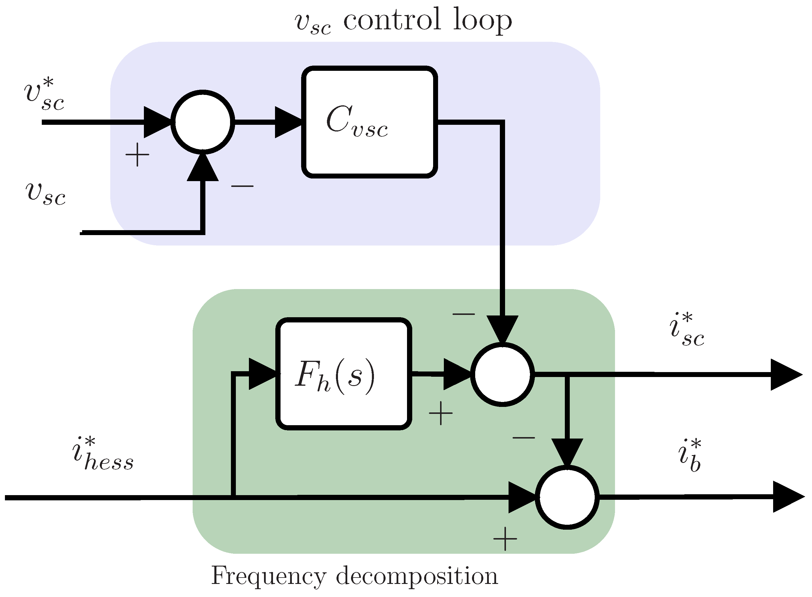
Figure 14.
Modified FBM with SC SoC.

Figure 15.
Unbalance current .

Figure 16.
RB case. Top: BSS and SC currents , . Bottom: SC SoC .

Figure 17.
COEF case. Top: BSS and SC currents , . Bottom: SC SoC .

Figure 18.
TVF case. Top: BSS and SC currents , . Bottom: SC SoC .

Figure 19.
LOOP case. Top: BSS and SC currents , . Bottom: SC SoC .

Figure 20.
BSS SoC evolution for RB, COEFF, TVF, and LOOP cases.

Figure 21.
HESS bus voltage evolution for RB, COEFF, TVF, and LOOP cases.


Table 1.
HESS topologies features comparison.
| Characteristic | Passive | Semi-Active | Full-Active |
|---|---|---|---|
| Complexity | Low | Medium | High |
| Efficiency | High | Medium | Low |
| Flexibility | Low | Medium | High |
| Cost | Low | Medium | High |
Table 2.
FLC rules summary. neg is for negative, pos is for positive, d is for discharge, c is for charge, while med is for medium [31].
Table 2.
FLC rules summary. neg is for negative, pos is for positive, d is for discharge, c is for charge, while med is for medium [31].
| / | High-Neg | Med-Neg | Small-Neg | Zero | Small-Pos | Med-Pos | High-Pos |
|---|---|---|---|---|---|---|---|
| low | high-c | med-c | med-c | slow-c | slow-c | slow-d | med-d |
| med | high-c | med-c | slow-c | zero | slow-d | med-d | high-d |
| high | med-c | slow-c | slow-c | slow-d | slow-d | high-d | high-d |
Table 3.
SC current reference definition according to [34].
Table 3.
SC current reference definition according to [34].
| Condition | |
|---|---|
| ∧ | |
| ∧ | |
| ∧ | |
| ∧ |
Table 4.
Sharing coefficient proposed in [24].
Table 4.
Sharing coefficient proposed in [24].
| BSS SoC | |
|---|---|
| 1 | |
| 0.6 | |
| 0.3 | |
| 0 |
Table 5.
Rule-based EMS according to [23].
Table 5.
Rule-based EMS according to [23].
| Condition and Equivalence to Figure 7 | |||
|---|---|---|---|
| (1) ∧ | |||
| (2) ∧ | |||
| (3) ∧ | |||
| (4) ∧ | |||
| (5) ∧ | |||
| (6) ∧ | |||
| (7) ∧ | |||
| (8) ∧ |
Table 6.
Rule-based EMS according to [35].
Table 6.
Rule-based EMS according to [35].
| Condition and Equivalence to Figure 7 | |||
|---|---|---|---|
| (1) ∧ | |||
| (2) ∧ | |||
| (3) ∧ | |||
| (4) ∧ | |||
| (5) ∧ | |||
| (6) ∧ | |||
| (7) ∧ | |||
| (8) ∧ | |||
| ∧ |
Table 7.
FLC rules summary for the proposal in [44]. neg is for negative, pos is for positive, d is for discharge, c is for charge, while med is for medium [31].
| / | High-Neg | Small-Neg | Med | Small-Pos | High-Pos |
|---|---|---|---|---|---|
| neg | small-pos | small-pos | small-pos | high-neg | high-neg |
| med | med | med | small-pos | med | small-pos |
| pos | med | high-pos | med | med | small-pos |
Table 8.
Parameter values for simulation.
| Parameter | Value |
|---|---|
| DC link capacitor | 2000 μF |
| DC–DC converter inductance | 500 μH |
| Li-on battery nominal voltage | 12 |
| Li-on battery rated capacity | 11 |
| Li-on battery initial SoC | 60% |
| Li-on battery SoC limits | %, % |
| Supercapacitor capacitance | 2 F |
| Supercapacitor rated voltage | 16 V |
| Supercapacitor initial voltage | 8.5 V |
| Supercapacitor SoC limits | %, % |
| DC bus voltage | 60 V |
| LPF time constant | s |
| PI constants for DC voltage loop | , |
| PI constants for BSS current loop | , |
| PI constants for SC current loop | , |
Table 9.
Summary of comparisons.
| Method | Advantages | Disadvantages |
|---|---|---|
| RB | Simplest implementation | Degradation of the BSS may be caused when SC SoC reaches the operational limits |
| COEFF | SC operates for longer periods and a softer transition is provided when reaching the SoC limits | BSS degradation can still be caused |
| TVF | SC provides high-frequency current components for longer periods, and less BSS degradation than in previous cases is expected | More complex implementation and stability proof. |
| LOOP | SC recovers the SoC continuously, which prevents BSS degradation | Larger use of the BSS. Additional procedures on the tuning of the added loops |
Publisher’s Note: MDPI stays neutral with regard to jurisdictional claims in published maps and institutional affiliations. |
© 2022 by the authors. Licensee MDPI, Basel, Switzerland. This article is an open access article distributed under the terms and conditions of the Creative Commons Attribution (CC BY) license (https://creativecommons.org/licenses/by/4.0/).
Share and Cite
MDPI and ACS Style
Ramos, G.A.; Costa-Castelló, R. Energy Management Strategies for Hybrid Energy Storage Systems Based on Filter Control: Analysis and Comparison. Electronics 2022, 11, 1631. https://0-doi-org.brum.beds.ac.uk/10.3390/electronics11101631
AMA Style
Ramos GA, Costa-Castelló R. Energy Management Strategies for Hybrid Energy Storage Systems Based on Filter Control: Analysis and Comparison. Electronics. 2022; 11(10):1631. https://0-doi-org.brum.beds.ac.uk/10.3390/electronics11101631
Chicago/Turabian StyleRamos, Germán Andrés, and Ramon Costa-Castelló. 2022. "Energy Management Strategies for Hybrid Energy Storage Systems Based on Filter Control: Analysis and Comparison" Electronics 11, no. 10: 1631. https://0-doi-org.brum.beds.ac.uk/10.3390/electronics11101631
Note that from the first issue of 2016, this journal uses article numbers instead of page numbers. See further details here.