
Improvement of the Performance of Models for Predicting Coronary Artery Disease Based on XGBoost Algorithm and Feature Processing Technology

Abstract
:1. Introduction
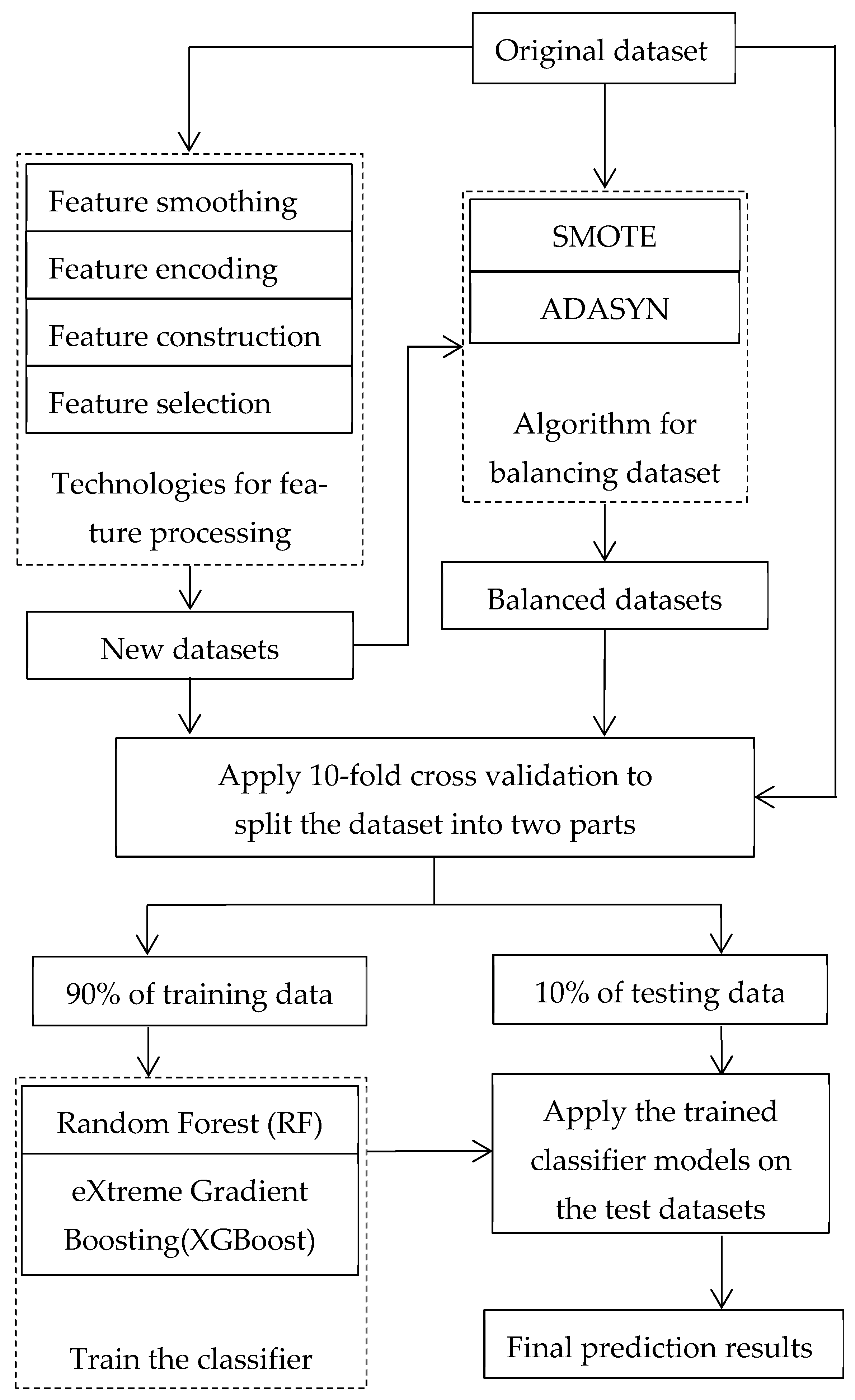
2. Proposed Method
2.1. Feature Processing Technologies
2.1.1. Feature Smoothing
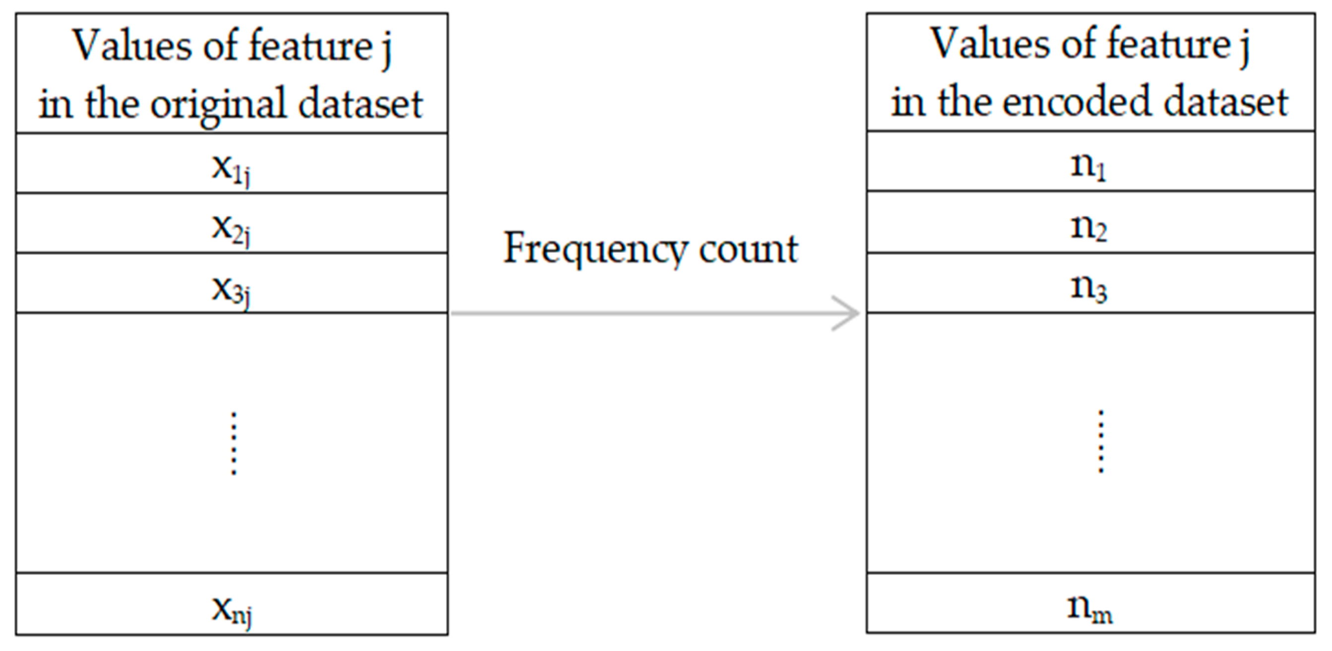
2.1.2. Feature Encoding
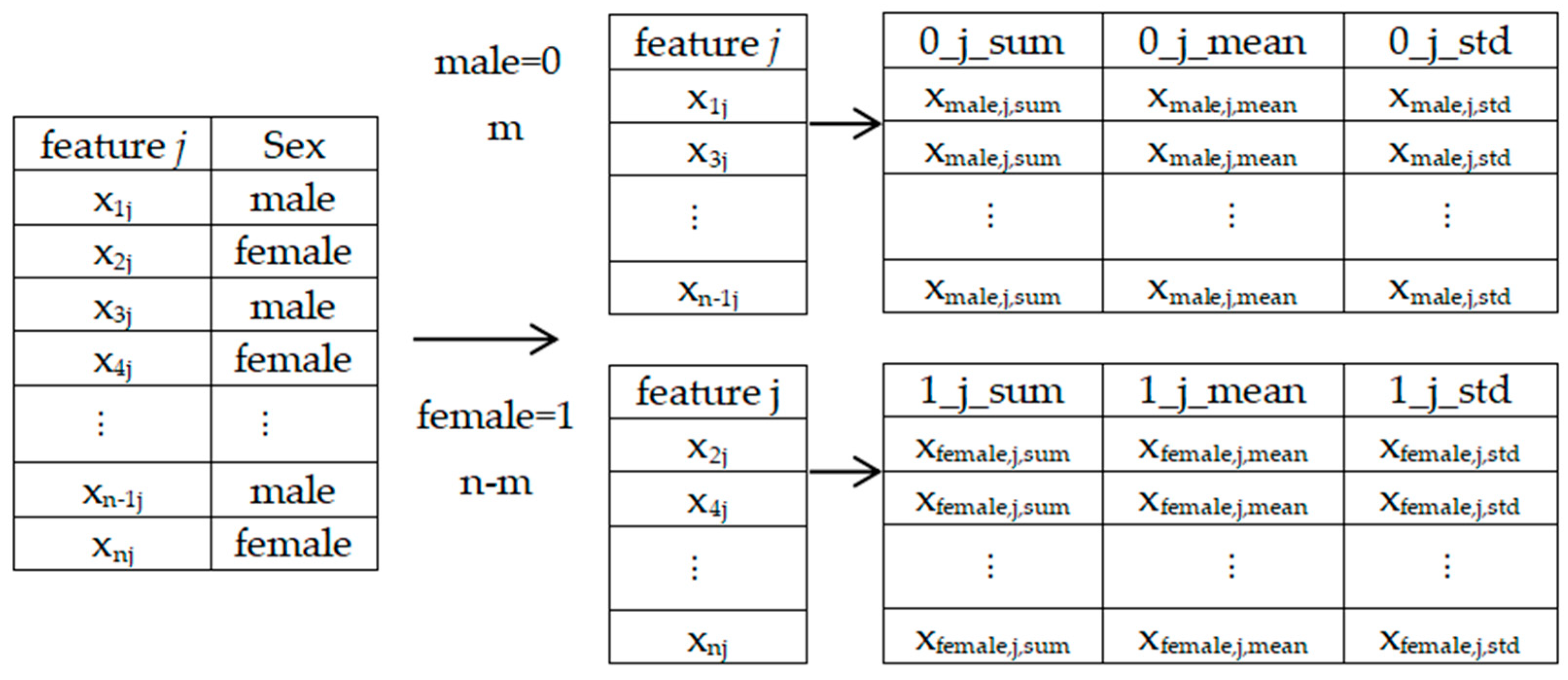
2.1.3. Feature Construction
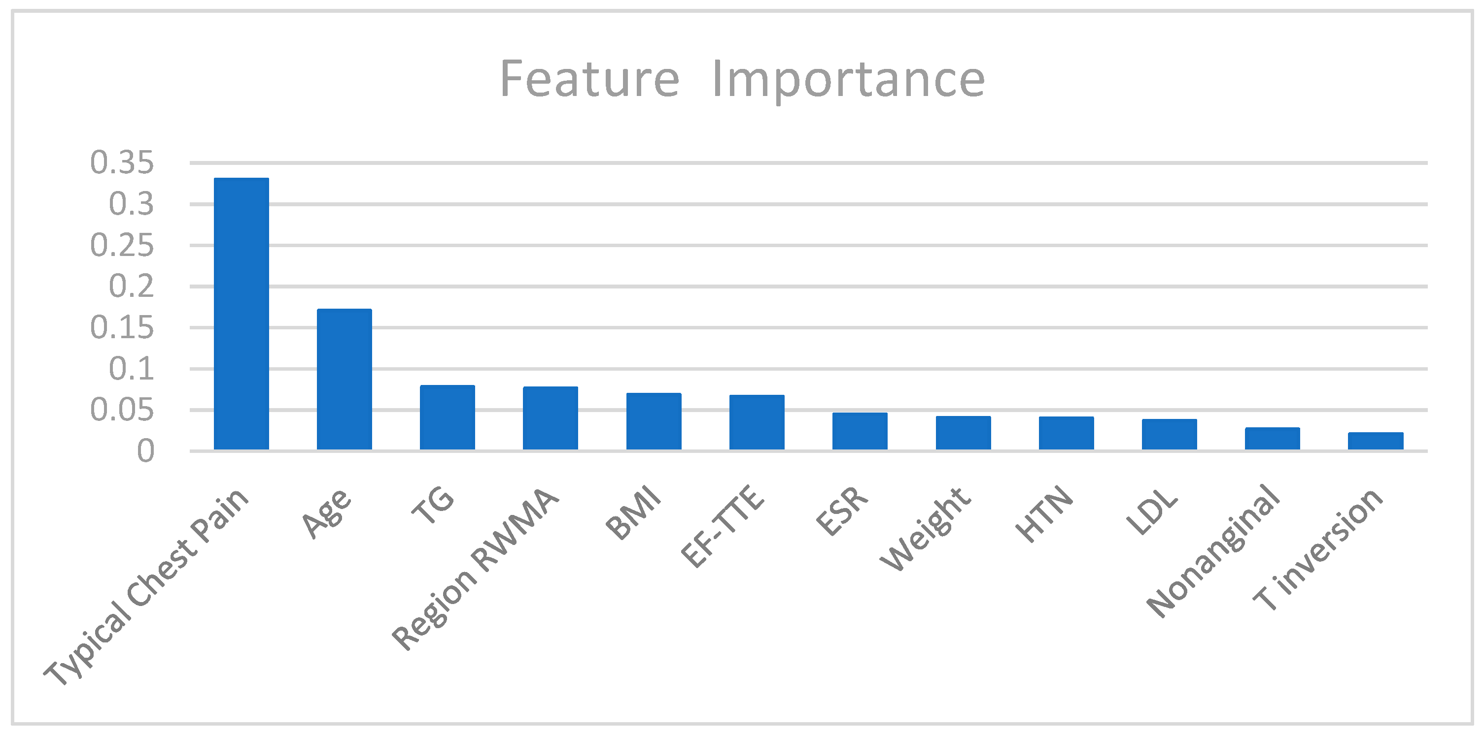
2.1.4. Feature Selection
2.2. Processing Method of Unbalanced Dataset
2.3. Classification Algorithm
3. Experiments and Results
3.1. Experimental Dataset
3.2. Evaluation Metrics
3.2.1. Confusion Matrix
3.2.2. Classification Metrics
- Accuracy
- 2.
- Precision
- 3.
- Recall
- 4.
- F1 score
- 5.
- Specificity
- 6.
- AUC
3.3. Experimental Results
3.3.1. Results Obtained on Original Dataset and Two Balanced Datasets
3.3.2. Results Obtained on Datasets Processed by Feature Smoothing and Two Dataset Balancing Methods
3.3.3. Results Obtained on Datasets Processed by Feature Encoding and Two Dataset Balancing Methods
3.3.4. Results Obtained on Datasets Processed by Feature Selection and Two Dataset Balancing Methods
3.3.5. Results Obtained on Datasets Processed by Feature Construction and Two Dataset Balancing Methods
4. Discussion
5. Conclusions
Author Contributions
Funding
Conflicts of Interest
References
- Mensah, G.A.; Roth, G.A.; Fuster, V. The Global Burden of Cardiovascular Diseases and Risk Factors 2020 and Beyond. JACC 2019, 74, 2529–2532. [Google Scholar] [CrossRef] [PubMed]
- GBD 2019 Risk Factors Collaborators. Global burden of 87 risk factors in 204 countries and territories, 1990–2019: A systematic analysis for the Global Burden of Disease Study 2019. Lancet 2020, 396, 1223–1249. [Google Scholar] [CrossRef]
- GBD 2019 Diseases and Injuries Collaborators. Global burden of 369 diseases and injuries in 204 countries and territories, 1990–2019: A systematic analysis for the Global Burden of Disease Study 2019. Lancet 2020, 396, 1204–1222. [Google Scholar] [CrossRef]
- Zipes, D.P.; Libby, P.; Bonow, R.O. Braunwald’s Heart Disease E-Book: A Textbook of Cardiovascular Medicine; Elsevier Health Sciences: Amsterdam, The Netherlands, 2018. [Google Scholar]
- Jayaraman, V.; Sultana, H.P. Artifificial gravitational cuckoo search algorithm along with particle bee optimized associative memory neural network for feature selection in heart disease classification. J. Ambient Intell. Humaniz. Comput. 2019, 1–10. [Google Scholar] [CrossRef]
- Liu, M.; Kim, Y. Classification of Heart Diseases Based on ECG Signals Using Long Short-Term Memory. In Proceedings of the 40th Annual International Conference of the IEEE Engineering in Medicine and Biology Society (EMBC), Honolulu, HI, USA, 18–21 July 2018; pp. 2707–2710. [Google Scholar]
- Vijayashree, J.; Sultana, H.P. Heart disease classification using hybridized ruzzo-tompa memetic based deep trained neocognitron neural network. Health Technol. 2019, 10, 207–216. [Google Scholar] [CrossRef]
- Alizadehsani, R.; Abdar, M.; Roshanzamir, M.; Khosravi, A.; Kebria, P.M.; Khozeimeh, F.; Nahavandi, S.; Sarrafzadegan, N.; Acharya, U.R. Machine learning-based coronary artery disease diagnosis: A comprehensive review. Comput. Biol. Med. 2019, 111, 103346. [Google Scholar] [CrossRef]
- Nasarian, E.; Abdar, M.; Fahami, M.A.; Alizadehsani, R.; Hussaind, S.; Basiri, M.E.; Zomorodi-Moghadam, M.; Zhou, X.J.; Pławiak, P.; Acharya, U.R.; et al. Association between work-related features and coronary artery disease: A heterogeneous hybrid feature selection integrated with balancing approach. Pattern Recognit. Lett. 2020, 133, 33–40. [Google Scholar] [CrossRef]
- Abdar, M.; Książek, W.; Acharya, U.R.; Tan, R.S.; Makarenkov, V.; Pławiak, P. A new machine learning technique for an accurate diagnosis of coronary artery disease. Comput. Methods Programs Biomed. 2019, 179, 104992. [Google Scholar] [CrossRef]
- Kolukisa, B.; Hacilar, H.; Goy, G.; Kus, M.; Bakir-Gungor, B.; Aral, A.; Gungor, V.C. Evaluation of Classification Algorithms, Linear Discriminant Analysis and a New Hybrid Feature Selection Methodology for the Diagnosis of Coronary Artery Disease. In Proceedings of the 2018 IEEE International Conference on Big Data (Big Data), Seattle, WA, USA, 10–13 December 2018; pp. 2232–2238. [Google Scholar]
- Zomorodi-moghadam, M.; Abdar, M.; Davarzani, Z.; Zhou, X.J.; Pławiak, P.; Acharya, U.R. Hybrid particle swarm optimization for rule discovery in the diagnosis of coronary artery disease. Expert Syst. 2019, 38, e12485. [Google Scholar] [CrossRef]
- Arabasadi, Z.; Alizadehsani, R.; Roshanzamir, M.; Moosaei, H.; Yarifard, A.A. Computer aided decision making for heart disease detection using hybrid neural network-Genetic algorithm. Comput. Methods Programs Biomed. 2017, 141, 19–26. [Google Scholar] [CrossRef]
- Joloudari, J.H.; Joloudari, E.H.; Saadatfar, H.; GhasemiGol, M.; Razavi, S.M.; Mosavi, A.; Nabipour, N.; Shamshirband, S.; Nadai, L. Coronary artery disease diagnosis; ranking the significant features using a random trees model. Int. J. Environ. Res. Public Health 2020, 17, 731. [Google Scholar] [CrossRef] [Green Version]
- Alizadehsani, R.; Habibi, J.; Hosseini, M.J.; Mashayekhi, H.; Boghrati, R.; Ghandeharioun, A.; Bahadorian, B.; Sani, Z.A. A data mining approach for diagnosis of coronary artery disease. Comput. Methods Programs Biomed. 2013, 111, 52–61. [Google Scholar] [CrossRef]
- Alizadehsani, R.; Hosseini, M.J.; Khosravi, A.; Khozeimeh, F.; Roshanzamir, M.; Sarrafzadegan, N.; Nahavandi, S. Non-invasive detection of coronary artery disease in high-risk patients based on the stenosis prediction of separate coronary arteries. Comput. Methods Programs Biomed. 2018, 162, 119–127. [Google Scholar] [CrossRef]
- Abdar, M.; Acharya, U.R.; Sarrafzadegan, N.; Makarenkov, V. Ne-nu-svc: A new nested ensemble clinical decision support system for effective diagnosis of coronary artery disease. IEEE Access 2019, 7, 167605–167620. [Google Scholar] [CrossRef]
- Ashish, L.; Kumar, S.; Yeligeti, S. Ischemic heart disease detection using support vector machine and extreme gradient boosting method. Mater. Today Proc. 2021. [Google Scholar] [CrossRef]
- Tian, Z.; Chen, C.Y.; Fan, Y.M.; Ou, X.J.; Wang, J.; Ma, X.L.; Xu, J.G. Glioblastoma and Anaplastic Astrocytoma: Differentiation Using MRI Texture Analysis. Front. Oncol. 2019, 9, 876. [Google Scholar] [CrossRef]
- Qing, Y.; Zhi, J.C.; Ying, L.T. Prediction of aptamer–protein interacting pairs based on sparse autoencoder feature extraction and an ensemble classifier. Math. Biosci. 2019, 311, 103–108. [Google Scholar] [CrossRef]
- Friedman, J.H. Greedy function approximation: A gradient boosting machine. Ann. Stat. 2001, 29, 1189–1232. [Google Scholar] [CrossRef]
- Liu, T.; Moore, A.W.; Gray, A.; Yang, K. An investigation of practical approximate nearest neighbor algorithms. In Proceedings of the 17th International Conference on Neural Information Processing Systems; MIT Press: Cambridge, MA, USA, 2004; pp. 825–832. [Google Scholar]
- Chawla, N.V.; Bowyer, K.W.; Hall, L.O.; Kegelmeyer, W.P. Smote: Synthetic minority over-sampling technique. J. Artif. Intell. Res. 2002, 16, 321–357. [Google Scholar] [CrossRef]
- Xu, X.L.; Chen, W.; Sun, Y.F. Over-sampling algorithm for imbalanced data classification. J. Syst. Eng. Electron. 2019, 30, 1182–1191. [Google Scholar] [CrossRef]
- Lee, H.S.; Jung, S.; Kim, M.; Kim, S. Synthetic Minority Over-Sampling Technique based on Fuzzy C-means Clustering for Imbalanced Data. In Proceedings of the 2017 International Conference on Fuzzy Theory and Its Applications (iFUZZY), Taiwan, China, 12–15 November 2017. [Google Scholar] [CrossRef]
- Gosain, A.; Sardana, S. Handling Class Imbalance Problem using Oversampling Techniques: A Review. In Proceedings of the 2017 International Conference on Advances in Computing, Communications and Informatics (ICACCI), Udupi, India, 13–16 September 2017; pp. 79–85. [Google Scholar] [CrossRef]
- He, H.; Bai, Y.; Garcia, E.A.; Li, S. Adasyn: Adaptive synthetic sampling approach for imbalanced learning. In Proceedings of the 2008 IEEE International Joint Conference on Neural Networks (IEEE World Congress on Computational Intelligence), Hong Kong, China, 1–6 June 2008; pp. 1322–1328. [Google Scholar]
- Satapathy, S.K.; Mishra, S.; Mallick, P.K.; Chae, G.S. ADASYN and ABC-optimized RBF convergence network for classification of electroencephalograph signal. Pers. Ubiquitous Comput. 2021, 1–17. [Google Scholar] [CrossRef]
- Breiman, L. Random forests. Mach. Learn. 2001, 45, 5–32. [Google Scholar] [CrossRef] [Green Version]
- Akyol, K.; Çalik, E.; Bayir, Ş.; Şen, B.; Çavuşoğlu, A. Analysis of demographic characteristics creating coronary artery disease susceptibility using random forests classifier. Procedia Comput. Sci. 2015, 62, 39–46. [Google Scholar] [CrossRef] [Green Version]
- Chen, T.; Guestrin, C. Xgboost: A scalable tree boosting system. In Proceedings of the 22nd Acm Sigkdd International Conference on Knowledge Discovery and Data Mining, San Francisco, CA, USA, 13–17 August 2016; ACM (Association for Computing Machinery) Digital Library: New York, NY, USA, 2016; pp. 785–794. [Google Scholar]
- Chen, Y.; Wang, X.; Jung, Y.; Abedi, V.; Zand, R.; Bikak, M.; Adibuzzaman, M. Classification of short single-lead electrocardiograms (ECGs) for atrial fibrillation detection using piecewise linear spline and XGBoost. Physiol. Meas. 2018, 39, 104006. [Google Scholar] [CrossRef]
- Torlay, L.; Perrone-Bertolotti, M.; Thomas, E.; Baciu, M. Machine learning–XGBoost analysis of language networks to classify patients with epilepsy. Brain Inf. 2017, 4, 159. [Google Scholar] [CrossRef]
- Van Rosendael, A.R.; Maliakal, G.; Kolli, K.K.; Beecy, A.; Al’Aref, S.J.; Dwivedi, A.; Singh, G.; Panday, M.; Kumar, A.; Ma, X.Y.; et al. Maximization of the usage of coronary CTA derived plaque information using a machine learning based algorithm to improve risk stratification; insights from the CONFIRM registry. J. Cardiovasc. Comput. Tomogr. 2018, 12, 204–209. [Google Scholar] [CrossRef]
- Alizadehsani, R.; Hosseini, M.J.; Sani, Z.A.; Ghandeharioun, A.; Boghrati, R. Diagnosis of coronary artery disease using cost-sensitive algorithms. In Proceedings of the IEEE 12th International Conference on Data Mining Workshops, Brussels, Belgium, 10 December 2012; pp. 9–16. [Google Scholar]
- Dekamin, A.; Sheibatolhamdi, A. A data mining approach for coronary artery disease prediction in Iran. J. Adv. Med. Sci. Appl. Technol. 2017, 3, 29–38. [Google Scholar] [CrossRef] [Green Version]
- Li, H.; Wang, X.P.; Li, Y.; Qin, C.J.; Liu, C.C. Comparison between medical knowledge based and computer automated feature selection for detection of coronary artery disease using imbalanced data. In Proceedings of the BIBE 2018, International Conference on Biological Information and Biomedical Engineering, Shanghai, China, 6–8 June 2018; pp. 1–4. [Google Scholar]
- Cüvitoğlu, A.; Işik, Z. Classification of cad dataset by using principal component analysis and machine learning approaches. In Proceedings of the 2018 5th International Conference on Electrical and Electronic Engineering (ICEEE), Istanbul, Turkey, 3–5 May 2018; pp. 340–343. [Google Scholar]
- Shahid, A.H.; Singh, M.P. A Novel Approach for Coronary Artery Disease Diagnosis using Hybrid Particle Swarm Optimization based Emotional Neural Network. Biocybern. Biomed. Eng. 2020, 40, 1568–1585. [Google Scholar] [CrossRef]


| Category | Feature Name | Range | Type |
|---|---|---|---|
| Demographic features | Age | 30–86 | continuous |
| Weight | 48–120 | continuous | |
| Length | 140–188 | continuous | |
| Sex | Male, Female | categorical | |
| BMI | 18.12–40.90 | continuous | |
| DM | 0, 1 | categorical | |
| HTN | 0, 1 | categorical | |
| Current smoker | 0, 1 | categorical | |
| Ex-smoker | 0, 1 | categorical | |
| FH | 0, 1 | categorical | |
| Obesity (Yes (BMI > 25), else No) | Y, N | categorical | |
| CRF | Y, N | categorical | |
| CVA | Y, N | categorical | |
| Airway disease | Y, N | categorical | |
| Thyroid disease | Y, N | categorical | |
| CHF | Y, N | categorical | |
| DLP | Y, N | categorical | |
| Symptoms and Physical examination | BP | 90.0–190.0 | continuous |
| PR | 50.0–110.0 | continuous | |
| Edema | 0, 1 | categorical | |
| Weak peripheral pulse | Y, N | categorical | |
| Lung rales | Y, N | categorical | |
| Systolic murmur | Y, N | categorical | |
| Diastolic murmur | Y, N | categorical | |
| Typical chest pain | 0, 1 | categorical | |
| Dyspnea | Y, N | categorical | |
| Function class | 1–4 | categorical | |
| Atypical | Y, N | categorical | |
| Nonanginal | Y, N | categorical | |
| Exertional CP | N | categorical | |
| LowTH Ang | Y, N | categorical | |
| Electrocardiography | Q Wave | 0, 1 | categorical |
| St elevation | 0, 1 | categorical | |
| St depression | 0, 1 | categorical | |
| T inversion | 0, 1 | categorical | |
| LVH | Y, N | categorical | |
| Poor R progression | Y, N | categorical | |
| BBB | N, LBBB, RBBB | categorical | |
| Laboratory Tests and Echocardiography | FBS | 62.0–400.0 | continuous |
| CR | 0.5–2.2 | continuous | |
| TG | 37.0–1050.0 | continuous | |
| LDL | 18.0–232.0 | continuous | |
| HDL | 15.9–111.0 | continuous | |
| BUN | 6.0–52.0 | continuous | |
| ESR | 1–90 | continuous | |
| HB | 8.9–17.6 | continuous | |
| K | 3.0–6.6 | continuous | |
| Na | 128.0–156.0 | continuous | |
| WBC | 3700–18,000 | continuous | |
| Lymph | 7.0–60.0 | continuous | |
| Neut | 32.0–89.0 | continuous | |
| PLT | 25.0–742.0 | continuous | |
| EF-TTE | 15.0–60.0 | continuous | |
| Region RWMA | 0, 1, 2, 3, 4 | categorical | |
| VHD | Mild, N, moderate, severe | categorical | |
| Cath_label | Cath |
| TN | FP | |
| FN | TP |
| Datasets | Algorithms | Recall | F1 | Accuracy | Precision | Specificity | AUC |
|---|---|---|---|---|---|---|---|
| Original data | Random Forest | 0.909 ± 0.051 | 0.923 ± 0.038 | 0.887 ± 0.056 | 0.940 ± 0.051 | 0.834 ± 0.117 | 0.92 ± 0.05 |
| XGBoost | 0.909 ± 0.072 | 0.929 ± 0.044 | 0.894 ± 0.068 | 0.954 ± 0.046 | 0.856 ± 0.106 | 0.93 ± 0.05 | |
| Balanced data with SMOTE | Random Forest | 0.939 ± 0.086 | 0.941 ± 0.045 | 0.938 ± 0.052 | 0.949 ± 0.044 | 0.936 ± 0.041 | 0.98 ± 0.03 |
| XGBoost | 0.940 ± 0.087 | 0.943 ± 0.044 | 0.940 ± 0.052 | 0.953 ± 0.037 | 0.940 ± 0.035 | 0.97 ± 0.03 | |
| Balanced data with ADASYN | Random Forest | 0.937 ± 0.081 | 0.930 ± 0.040 | 0.928 ±0.045 | 0.930 ± 0.048 | 0.918 ± 0.041 | 0.96 ± 0.04 |
| XGBoost | 0.939 ± 0.082 | 0.942 ± 0.042 | 0.939 ± 0.048 | 0.953 ± 0.048 | 0.941 ± 0.096 | 0.97 ± 0.03 |
| Datasets | Algorithms | Recall | F1 | Accuracy | Precision | Specificity | AUC |
|---|---|---|---|---|---|---|---|
| Data processed by feature smoothing | Random Forest | 0.892 ± 0.051 | 0.922 ± 0.033 | 0.884 ± 0.053 | 0.958 ± 0.039 | 0.866 ± 0.094 | 0.91 ± 0.06 |
| XGBoost | 0.914 ± 0.070 | 0.931 ± 0.037 | 0.898 ± 0.059 | 0.954 ± 0.046 | 0.857 ± 0.100 | 0.93 ± 0.06 | |
| Data processed by feature smoothing and SMOTE | Random Forest | 0.939 ± 0.081 | 0.933 ± 0.046 | 0.931 ± 0.051 | 0.931 ± 0.031 | 0.923 ± 0.033 | 0.98 ± 0.02 |
| XGBoost | 0.945 ± 0.083 | 0.935 ± 0.046 | 0.933 ± 0.053 | 0.930 ± 0.038 | 0.921 ± 0.040 | 0.98 ± 0.02 | |
| Data processed by feature smoothing and ADASYN | Random Forest | 0.936 ± 0.087 | 0.936 ± 0.052 | 0.932 ± 0.059 | 0.940 ± 0.036 | 0.928 ± 0.041 | 0.98 ± 0.02 |
| XGBoost | 0.941 ± 0.078 | 0.942 ± 0.041 | 0.939 ± 0.045 | 0.948 ± 0.045 | 0.937 ± 0.040 | 0.97 ± 0.03 |
| Datasets | Algorithms | Recall | F1 | Accuracy | Precision | Specificity | AUC |
|---|---|---|---|---|---|---|---|
| Data processed by feature encoding | Random Forest | 0.900 ± 0.058 | 0.920 ± 0.027 | 0.881 ± 0.046 | 0.944 ± 0.041 | 0.833 ± 0.070 | 0.91 ± 0.06 |
| XGBoost | 0.918 ± 0.053 | 0.925 ± 0.032 | 0.891 ± 0.047 | 0.935 ± 0.047 | 0.824 ± 0.101 | 0.93 ± 0.06 | |
| Data processed by feature encoding and SMOTE | Random Forest | 0.949 ± 0.071 | 0.933 ± 0.035 | 0.933 ± 0.037 | 0.925 ± 0.065 | 0.917 ± 0.056 | 0.98 ± 0.01 |
| XGBoost | 0.943 ± 0.075 | 0.932 ± 0.037 | 0.931 ± 0.041 | 0.926 ± 0.037 | 0.918 ± 0.030 | 0.97 ± 0.02 | |
| Data processed by feature encoding and ADASYN | Random Forest | 0.924 ± 0.081 | 0.926 ± 0.040 | 0.922 ± 0.047 | 0.935 ± 0.043 | 0.919 ± 0.038 | 0.96 ± 0.03 |
| XGBoost | 0.933 ± 0.084 | 0.928 ± 0.042 | 0.924 ± 0.048 | 0.930 ± 0.043 | 0.915 ± 0.039 | 0.97 ± 0.03 |
| Feature_Name | Importance 1 |
|---|---|
| Typical chest pain | 0.329970 |
| Age | 0.170756 |
| TG | 0.077998 |
| Region RWMA | 0.076567 |
| BMI | 0.068513 |
| EF-TTE | 0.066505 |
| ESR | 0.044726 |
| Weight | 0.040609 |
| HTN | 0.039968 |
| LDL | 0.037006 |
| Nonanginal | 0.026549 |
| T inversion | 0.020833 |
| Datasets | Algorithms | Recall | F1 | Accuracy | Precision | Specificity | AUC |
|---|---|---|---|---|---|---|---|
| Data processed by feature selection | Random Forest | 0.899 ± 0.067 | 0.930 ± 0.039 | 0.894 ± 0.062 | 0.968 ± 0.036 | 0.884 ± 0.091 | 0.95 ± 0.04 |
| XGBoost | 0.927 ± 0.058 | 0.939 ± 0.039 | 0.911 ± 0.057 | 0.954 ± 0.054 | 0.870 ± 0.127 | 0.94 ± 0.05 | |
| Data processed by feature selection and SMOTE | Random Forest | 0.944 ± 0.075 | 0.937 ± 0.037 | 0.935 ± 0.042 | 0.935 ± 0.043 | 0.927 ± 0.040 | 0.97 ± 0.03 |
| XGBoost | 0.943 ± 0.079 | 0.942 ± 0.052 | 0.940 ± 0.056 | 0.944 ± 0.046 | 0.937 ± 0.050 | 0.96 ± 0.04 | |
| Data processed by feature selection and ADASYN | Random Forest | 0.944 ± 0.073 | 0.941 ± 0.038 | 0.939 ± 0.042 | 0.944 ± 0.051 | 0.935 ± 0.047 | 0.97 ± 0.02 |
| XGBoost | 0.946 ± 0.067 | 0.943 ± 0.040 | 0.942 ± 0.043 | 0.944 ± 0.041 | 0.938 ± 0.042 | 0.97 ± 0.04 |
| Datasets | Algorithms | Recall | F1 | Accuracy | Precision | Specificity | AUC |
|---|---|---|---|---|---|---|---|
| Data processed by feature construction | Random Forest | 0.897 ± 0.072 | 0.918 ± 0.040 | 0.878 ± 0.064 | 0.944 ± 0.035 | 0.829 ± 0.089 | 0.90 ± 0.06 |
| XGBoost | 0.911 ± 0.073 | 0.929 ± 0.036 | 0.895 ± 0.059 | 0.954 ± 0.041 | 0.854 ± 0.090 | 0.93 ± 0.05 | |
| Data processed by feature construction and SMOTE | Random Forest | 0.933 ± 0.085 | 0.934 ± 0.046 | 0.931 ± 0.051 | 0.940 ± 0.037 | 0.929 ± 0.035 | 0.97 ± 0.03 |
| XGBoost | 0.961 ± 0.048 | 0.946 ± 0.030 | 0.947 ± 0.029 | 0.934 ± 0.053 | 0.932 ± 0.049 | 0.98 ± 0.02 | |
| Data processed by feature construction and ADASYN | Random Forest | 0.933 ± 0.088 | 0.921 ± 0.048 | 0.917 ± 0.057 | 0.916 ± 0.051 | 0.899 ± 0.052 | 0.96 ± 0.04 |
| XGBoost | 0.946 ± 0.065 | 0.938 ± 0.037 | 0.936 ± 0.041 | 0.935 ± 0.043 | 0.925 ± 0.044 | 0.98 ± 0.02 |
| Method | Feature Nums | Accuracy % | Recall % | Specificity % | Precision % | F1% | AUC |
|---|---|---|---|---|---|---|---|
| SMO [35] | 34 | 92.09 | 97.22 | 79.31 | NR | NR | NR |
| SMO + information gain [15] | 33 | 94.08 | 96.30 | 88.51 | NR | NR | NR |
| KNN (K1 KNN) [36] | NR | 90.91 | 93.33 | 85.71 | 93.33 | 93.33 | NR |
| NN + genetic [13] | 22 | 93.85 | 97 | 92 | NR | NR | NR |
| NB + genetic algorithm [37] | 32 | 88.16 | 88.00 | 87.78 | NR | NR | NR |
| Ensemble [38] | 25 | 86.49 | 73.61 | 91.67 | NR | 0.75 | 0.83 |
| SVM + feature engineering [16] | 28 | 96.4 | 100 | 88.1 | NR | NR | 0.92 |
| NE-nu-SVC [17] | 16 | 94.66 | 94.70 | NR | 94.70 | 94.70 | 0.966 |
| N2GC-nuSVM [10] | 29 | 93.08 | NR | NR | NR | 91.51 | NR |
| XGBoost + hybrid FSA + FA + ETCA + SMOTE [9] | 27 | 92.58 | 92.99 | NR | 92.59 | 90.62 | NR |
| Hybrid PSO-EmNN coupled with feature selection [39] | 22 | 88.34 | 91.85 | 78.98 | 92.37 | 92.12 | NR |
| XGBoost + GDBT + ADASYN * | 12 | 94.2 | 94.6 | 93.8 | 94.4 | 94.3 | 0.97 |
| XGBoost + feature construction + SMOTE * | 120 | 94.7 | 96.1 | 93.2 | 93.4 | 94.6 | 0.98 |
Publisher’s Note: MDPI stays neutral with regard to jurisdictional claims in published maps and institutional affiliations. |
© 2022 by the authors. Licensee MDPI, Basel, Switzerland. This article is an open access article distributed under the terms and conditions of the Creative Commons Attribution (CC BY) license (https://creativecommons.org/licenses/by/4.0/).
Share and Cite
Zhang, S.; Yuan, Y.; Yao, Z.; Wang, X.; Lei, Z. Improvement of the Performance of Models for Predicting Coronary Artery Disease Based on XGBoost Algorithm and Feature Processing Technology. Electronics 2022, 11, 315. https://0-doi-org.brum.beds.ac.uk/10.3390/electronics11030315
Zhang S, Yuan Y, Yao Z, Wang X, Lei Z. Improvement of the Performance of Models for Predicting Coronary Artery Disease Based on XGBoost Algorithm and Feature Processing Technology. Electronics. 2022; 11(3):315. https://0-doi-org.brum.beds.ac.uk/10.3390/electronics11030315
Chicago/Turabian StyleZhang, Shasha, Yuyu Yuan, Zhonghua Yao, Xinyan Wang, and Zhen Lei. 2022. "Improvement of the Performance of Models for Predicting Coronary Artery Disease Based on XGBoost Algorithm and Feature Processing Technology" Electronics 11, no. 3: 315. https://0-doi-org.brum.beds.ac.uk/10.3390/electronics11030315