
Assessment of the Current for a Non-Linear Power Inductor Including Temperature in DC-DC Converters


1
Department of Engineering, University of Palermo, 90128 Palermo, Italy
2
ICAR—Institute for High Performance Computing and Networking, National Research Council (CNR), Via Ugo La Malfa, 153, 90146 Palermo, Italy
*
Author to whom correspondence should be addressed.
Electronics 2023, 12(3), 579; https://0-doi-org.brum.beds.ac.uk/10.3390/electronics12030579
Submission received: 28 December 2022
/
Revised: 13 January 2023
/
Accepted: 19 January 2023
/
Published: 24 January 2023
(This article belongs to the Special Issue Power Electronics in Italy—Emerging Electronic Power Technologies and Electronic Devices in the Industrial 4.0 Era)
Abstract
:A method for estimating the current flowing through a non-linear power inductor operating in a DC/DC converter is proposed. The knowledge of such current, that cannot be calculated in closed form as for the linear inductor, is crucial for the design of the converter. The proposed method is based on a third-order polynomial model of the inductor, already developed by the authors; it is exploited to solve the differential equation of the inductor and to implement a flux model in a circuit simulator. The method allows the estimation of the current up to saturation, intended as the point at which the differential inductance is reduced to half of its maximum value. The current profile depends also on the inductor temperature. Based on this, the influence of core temperature on the conduction time of the power switch was determined. This study shows that the exploitation of saturation requires a proper value of the conduction time value that depends on the temperature. The theoretical analysis has been experimentally verified on a boost converter and is valid for the entire class of DC-DC converters in which the power inductor is subjected to a constant voltage for a given time. The simulations agree with the experimental data from a case study concerning conduction time and temperature.
1. Introduction
Using a power inductor beyond the linear zone is of interest in modern power electronics because its exploitation improves the power density of switch-mode power supplies (SMPS); it allows a higher operating current without increasing the core size [1,2,3,4,5]. However, the different shape of the current, compared to a linear inductor, implies an increase in the current peak that rises the losses and, consequently, the operating temperature of the magnetic core [6]. For these reasons, knowledge of the current waveform is essential.
The non-linear behavior of the devices employed in a switching converter (including switches and passive devices) is of scientific interest since they can induce a chaotic behavior. In this case, the dynamic behavior changes from a well-recognizable steady state up to chaos represented by the loss of the period of the current through the inductance [7,8]; therefore, the trajectory in the plane “output voltage” versus “inductance current” does not overlap with itself for each switching period.
The core material of the inductor significantly contributes to saturation. Ferrites are widely used for inductor cores in power electronics; however, they provide an abrupt decrease in the inductance, emphasizing the increase in the current and temperature when the inductor is operated outside the linear zone [2,9]. The saturation, or pratical limit for the inductance, is defined as the point where the differential inductance is halved f(Lsat) compared to its rated maximum value [2], and depends on the magnetic core temperature [10]. Therefore, characterizing the thermal behavior is of paramount importance for the designer [10,11,12,13]. The current peak is strictly correlated with the conduction time of the power switch (TON) because the current through the inductor usually reaches its maximum value at the end of the TON. Hence, the knowledge of the current profile allows for avoiding overcurrent and preserving both the inductor and power switch.
Calculating the current peak based on the TON in SMPSs with a linear inductor is straightforward; contrarily, when the inductor works outside the linear zone, the analysis is more complicated because of non-linearity and temperature dependence.
The analysis of the current waveform up to the saturation point, is essential in the SMPS to perform the non-linear inductor design. On the contrary, deep saturation is unworthy because of the excessively low value of inductance Ldeepsat. The value of Lsat is often lacking in the manufacturers’ datasheet, where saturation is often considered to be the point at which the inductance is reduced by 10% only. For these reasons, a suitable characterization by a test rig was performed to retrieve a complete knowledge of the inductor [14]. Furthermore, the knowledge of the inductor-saturated model is particularly important for implementing virtual sensors or control actions that allow the estimation of the inductor current [15].
Concerning power electronics applications, a non-linear inductor can be conveniently employed for current in the region between zero and the saturation current which corresponds to the value when the inductance is reduced to one-half of the rated inductance. For this reason, the modeling of the whole hysteresis cycle is not required. It allows for simplifying the model of the inductor aiming for a low computational effort. In fact, a complete description of the hysteresis (useful in general to model, control, or to the identification of dynamical systems) would require an approach such as Preisach, Krasnosel’skii—Pokrovs-kii (KP), or Prandtl—Ishlinskii(PI) [16]. These methods are helpful in designing the control system (Feedforward control with open-loop schemes or Close-loop control with feedback information) when the hysteresis cycle is fully exploited (corresponding to the operation in all quadrants in the plane flux vs. current).
The study presented in this paper proposes a novel method for calculating the current profile flowing through a non-linear inductor subjected to a constant voltage for a given time interval. It is based on a suitable power inductor model up to saturation. The model encompasses the temperature, as the rise of temperature in the core causes a further lowering of inductance with a consequent increase in current, losses [17,18,19], and potential thermal runaway [10,20,21,22]. The polynomial curve satisfies the constraint to reproduce the inductance in the operating region; moreover, this model is computationally light, therefore the current can be calculated in a time shorter than the power switch’s conduction time. In this way, a simulator can evaluate the current (including the expected maximum value) before the next TON time is completed. This time interval imposes the computation time threshold, and it is crucial, especially for converters operated with very high switching frequency (adopting, as an example, GaN devices) where the switching period is reduced.
In our paper, we consider the design of a converter in which the current peak must be calculated to appropriately select the power switch and diode. Furthermore, we adopt and exploit a polynomial model to solve the differential equation of the inductor. This model is valid in a limited part of the plane inductance vs. current; however, it corresponds to the operating region in which the inductor behavior must be analyzed.
The main novelty of this paper consists of the exploitation of the polynomial inductor model to solve the differential equation of the non-linear inductor and to implement the flux model in closed form within a circuit simulator. The model has been previously developed [14]; here it is used to carry out the current shape. It is also of interest to industry, since it addresses the design based on the knowledge of the maximum current flowing through the inductor that flows through the power switch as well.
It should be noted that the inductor characterization using the proposed model can be extended to different core materials because the model is analytical and considers a function that approximates the magnetization curve.
The main models proposed in the literature are arctan [1] and polynomial models [14]. The two models provide a different approach that can be recognized depending on the desired trade-off between the accuracy and calculation resources [23,24]. A polynomial model was used in this study.
Among the other analytical models, summarized by [25], the neural model proposed in [26] provides very good results with few hidden neurons; however, the learning dataset required 250 points provided by manufacturers at a constant temperature. The piecewise-affine formulation [27] improves the use of the computational resources of [28]. In general, the so-called local approaches adopt different approximations depending on the current; the main disadvantage is the discontinuity of the inductance curve; therefore, this approach can be used only for small current variations.
The exploitation of the proposed model to solve the differential equation of a non-linear inductor and to implement the flux model in a closed form within a circuit simulator allows calculating the current profiles analytically and through simulations where an original flux model of the inductor is implemented in closed form. In addition, our analysis explains how the non-linear behavior of the inductor can be exploited when the duty cycle of an SMPS varies during operation, which strengthens the simplified approaches proposed by [1,27,28], where the current profile is given only in steady-state conditions, where the duty cycle is constant. In fact, a slight increase in TON under these operating conditions would also imply an unacceptable current increase or deep saturation of the inductor. In contrast, diminishing TON leads to an inductor in the linear zone, eliminating non-linear exploitation. Therefore, we demonstrated the need to tune the TON value and calculate the maximum TON, considering the temperature for a given current [29].
In general, the temperature can be assumed to be constant within a switching period. Hence, a model of the inductor taken at a given temperature is suitable for reproducing the current waveform once the temperature is known. However, during operation, the inductor experiences a slow thermal transient with a time constant on the order of minutes; during this time, the inductance varies. Therefore, the variation in inductance with temperature must be considered in the model [10,24]. We show how the adopted approach allows describing the current that varies because of the temperature. Finally, since the current through the inductor influences electromagnetic interference (EMI) [30], the spectrum and the root mean square of the current were also evaluated.
The remainder of this paper is organized as follows. The fundamentals of the model adopted for the inductor are summarized in Section 2. Section 3 describes the main theoretical contribution, that is, the algorithm for the current evaluation. The characterization of the inductor used for the experimental verification is briefly recalled in Section 4, and the boost converter for the experimental verification of the current profiles by varying the conduction time and temperature is proposed in Section 5. Finally, Section 6 compares the experimental results with the theoretical values obtained by the proposed method.
2. Analytical Model of the Non-Linear Inductor
The use of a power inductor up to the saturation region implies the need to manage a rapid decrease in the inductance value when saturation is approached, which causes a faster increase in the current than in a linear inductor. In fact, for a given voltage, the product of the inductance and current derivatives must remain constant. Exploitation requires a suitable model to forecast operations near saturation where a high current peak can be reached. This phenomenon could be attributed to the magnetic core material. Among the most used materials for power inductor cores, ferrite or iron powder cores are considered owing to their low power losses, high saturation induction, and low cost [31]; however, they exhibit a sharp transition from regions of low and deep saturation.
In this study, the inductor was modeled by a polynomial function following the approach proposed in [10], which includes saturation to model saturable reactors [29] because it revealed computationally light. A third-order polynomial provides a good approximation for practical applications [10]. In contrast to saturable reactors operated in AC, the power inductors used in SMPSs operate with a DC offset and superimposed AC signal; therefore, a suitable characterization system is required [14]. To include the temperature dependence in the model, polynomial coefficients were considered linearly dependent on the temperature, meaning that the magnetic flux for a given magnetizing current depends linearly on the temperature. Such a characterization is described in [32,33] in terms of the saturation flux, showing a very good approximate trend with a straight line for the practical temperature range (25–125 °C). Moreover, we experimentally verified this behavior in the inductor under study. The inductance is modeled as:
where Lm are polynomial coefficients and the linear dependence of the inductor temperature Tcore (°C) is described by the proportionality factors βm. The parameter Ldeepsat represents the inductance value when hard saturation is reached. The first term in (1) models the thermal behavior when the inductance is linear. Once the coefficients of (1) are known, the model can be easily implemented and requires fewer calculation resources compared, as an example, with a model based on hyperbolic functions. In addition, (1) shows a continuous derivative in the practical operating region. The coefficients Lm, βm, and Ldeepsat must be identified; they are obtained experimentally using the method proposed in [14] and briefly explained in Section 4.
3. Current Profile Calculation
In this study, an experimental analysis was performed on a boost converter, in which the power inductor was subjected to a DC supply voltage for a time interval imposed by the conduction (TON) of the power switch. This can be generalized to any SMPSs by considering an appropriate voltage value applied to the inductor.
In a boost converter (see Figure 1) with a linear inductor operated in continuous current mode (CCM), the current flowing through the inductor exhibits a triangular shape, and the current variation can be easily calculated. When the inductor is exploited outside the linear region, the current differs from the well-known triangular waveform, and its time derivative increases with time. Indeed, from the constitutive equation of the inductor , it can be deduced that a reduction in inductance implies an increase in the current derivative when the voltage vL at the inductor terminals is constant. In addition, the inductance drop in the saturation region is highly dependent on the magnetic core temperature.
Figure 2 compares the current waveforms for two different inductors (linear and non-linear) with the same load. The mean value of the current does not vary because it depends on the load. Moreover, the two areas defined by the non-linear curve under and over the mean value and mean value must be the same. Given the upward concavity of the current waveform for the non-linear inductor, the minimum value of current iLnl,min decreases. However, the current peak iLnl,max increased more than that of the previous decrease. It is worth noting that the current variation in the non-linear case ΔiLnl, is higher than the value observed in the linear case ΔiL.
When the inductance varies with the current, the relationship between inductor voltage and flux Φ must be considered.
Then, taking into account that temperature, Tcore, shows a slow variation (practically, the temperature remains constant during a switching period, as the latter is much shorter than the system thermal constant), (2) gives:
Equation (3) can be solved numerically: considering that the voltage applied to the inductor is constant,
Equation (4) follows the Euler method to simplify this description. However, in our simulations, the fourth-order Runge-Kutta method was used to achieve better accuracy. Equation (4) requires a starting condition, such as the value of the current at the beginning or at the end of the conduction time. In this case, the current peak value, that is, the current value when t = TON, is used as a starting point because this current peak is known because it is imposed by the design (i.e., the current at which the inductance is halved to fully exploit saturation). Therefore, the waveform of iL during the conduction time was obtained by evaluating (4), starting from t = TON and proceeding backward until t = 0.
Equation (3) can be solved through SPICE simulations, for example, using the POLY keyword implemented in SPICE 2G6 [33] or, by expressing the behavioral inductance specified with an expression for the flux in the LTspice simulator. The expression of the flux can be easily retrieved in closed form by integrating (3) through the polynomial model (1), as follows:
Equation (6) describes the flux model in a non-linear inductor modeled using a polynomial model. It should be noted that the 3rd-order polynomial model provides a good approximation when the inductor is operated up to the saturation limit previously defined (50% of the nominal inductance). However, it is still far from deep saturation, which is described by the constant value . As an alternative, the deep-saturation region can be modeled with a higher-order polynomial; however, this is not of interest for power electronic applications.
This study implements and compares both methods, that is, a simplified approach involving fourth-order Runge-Kutta to solve (3) and the circuital SPICE simulation (which uses the modified trap integration) implementing the behavioral flux model (6). In both methods, the losses in the inductor are considered and modeled using a suitable series resistance [10]. In this way, losses are considered without the need for complicated hysteresis modeling.
The reliability of circuit-level simulation in SPICE depends on several factors such as the numerical stability of integration, precision of results and convergence at each time step, and adequacy of device modeling. Most SPICE implementations follow Berkeley SPICE and provide two forms of second-order implicit integration which are Gear and Trapezoidal which are both A-stable. The trapezoidal is both faster and more accurate than Gear, however, it can give rise to a numerical artifact (ringing) [34]. The software used for the simulations of this paper is LTspice, it implements a proprietary algorithm called Modified-trap that exhibits the speed and accuracy of trapezoidal avoiding traditional trap ringing. The set of nonlinear equations is replaced through implicit integration in a set of time-independent nonlinear equations that are solved by the Newton-Raphson technique. For a given circuit, the numerical stability of integration depends on the integration formula being used and the size of the discretized time step; in situations presenting high Q or for stiff problems, convergence failure can occur [34]. However, for a boost converter and the transient simulation, like the ones presented in this paper, the convergence is less of a problem because the initial state of the capacitors and inductors is known, and precision problems can be limited by reducing the granularity of time discretization. Butusov et al. [35] have shown that nonlinear integration techniques based on Padè approximation to the chaotic system simulation significantly change the behavior of discrete models of nonlinear systems, increasing the values of Lyapunov exponents and spectral entropy. The authors are aware that the controlled DC/DC converters can originate a chaotic behavior [8,36]; to avoid this, the experiment is conducted in an open loop. In this way, the system presents a clear and stable steady state and the analysis can be focused only on the non-linearity of the inductor.
4. Inductor Characterization
The inductor was characterized using a dedicated electronic circuit controlled by a virtual instrument developed in LabVIEW®. A complete description of the characterization system can be found in [14]; here, only the fundamentals are given. The inductor under the test was placed in a DC/DC converter with a variable active load. The LabVIEW instrument imposes a switching frequency, duty cycle of the power switch, and DC bias current by varying the load. Finally, it calculates inductance L using the ratio between the voltage applied to the inductor (maintained constant) and the slope of the current:
A digital oscilloscope sampled the voltage and current on the inductor, whereas a thermocouple placed on the inductor measured its temperature. Thus, the inductance versus current curve for a given temperature was calculated. It should be noted that the temperature remained relatively uniform in this type of inductor; therefore, a thermostatic chamber was not required [10]. Before applying (7), the voltage drop due to parasitic resistance is calculated such that vL is the effective voltage applied to the inductor without parasitic resistive voltage drop. This avoids the fact that the error is crucial, particularly for high currents. The automatic system measures inductance based on (7) by increasing the current to saturation. Each measurement was performed while maintaining a constant temperature of the inductor. The polynomial model described by (1) was then retrieved by interpolation. The output of this procedure consists of the coefficients used to model inductors Lm and βm, and the deep saturation value Ldeepsat. To avoid that noise corrupting the evaluation of the current derivative, the measurement was repeated many times, calculating the average and standard deviation, corresponding to the true value and error, respectively. Based on the propagation error formula applied in (7), it can be noted that the error ΔL on the value of L decreases when the derivative increases, that is, for the values of the inductance outside the linear region:
where, for the sake of clarity, DiL indicates the time derivative of the current in the denominator of (8).
The inductor under test was a commercial Panasonic ELC18B221L ferrite core inductor (LNOMINAL 220 µH). This component was characterized by the system described in [14] and summarized in Section 4, and the coefficients of (1) were obtained and are summarized in Table 1. The experimental dataset and the corresponding polynomial model are compared in Figure 3.
5. The Boost Converter Used as Case Study
The inductor under test was a commercial Panasonic ELC18B221L ferrite core inductor (LNOMINAL 220 µH). The converter employed for the validation was a boost supplied by Vs = 24 V, and the switching frequency FS was equal to 30 kHz. It adopts an FDP12N60NZ MOSFET as the switch and a rectifier diode, STTH806. It has been loaded with a resistance of 20 Ω, and the output capacitance is equal to 33 μF. These values allow us to reach a maximum current of about 5 A, which is beyond the saturation limit (as noticeable from Figure 3), assessing that it is possible to extend the working operating range of a linear inductor with a suitable analysis. In fact, the rated current of the inductor is 2.4 A. Besides, an inductor with a rated current of about 5A operated in linear conditions would require a bigger, and more expensive, core. All measurements have been performed with a digital oscilloscope with a sample rate of 1 GS/s. The test rig used for the measurements is shown in Figure 4a and depicted in a pictorial diagram in Figure 4b. The test rig is controlled by a PC able to deliver the duty cycle based on the required maximum current and magnetic core temperature.
The following two measurements, given as examples, show the influence of TON on the inductor current peak. Figure 5 shows oscilloscope plots of the measurements performed on the current flowing through the MOSFET. The current was measured using a current probe TEKTRONIK TCP0020. The converter was operated in the CCM. Figure 5a, corresponding to TON = 15 μs, shows a linear current, whereas Figure 5b, corresponding to TON = 17 μs, shows a non-linear effect owed to the inductor. It is remarkable that a 13% increase in TON caused a 57% rise in the AC current peak; it increased from 0.81 A to 1.27 A, shifting the inductor operation from the linear to the non-linear zone.
Even if the increase of duty cycle (D) always leads to a rise of the current peak also in the case of a linear inductor, with a non-linear device this increase is more relevant. Besides, by adopting a linear inductor, the current peak can be easily calculated since the current variation is proportional to D:
In the case of the non-linear inductor, Equation (9) cannot be used since increasing the current, the inductance decreases leading to a further increase of the same current. Instead, the differential equation of the inductor must be solved by adopting the model as proposed in this paper.
We focused the attention on the current peak since it also stresses the power switch and affects its reliability. Once demonstrated that the non-linear operation of an inductor modifies the shape of the current, which is no longer triangular as in the case of a linear inductor, and implies a higher peak, richer harmonic content, and non-linear dependence on conduction time and temperature, there is a need to calculate the current shape.
In general, in non-linear operation, the peak depends on the duty cycle (or on TON) and on the temperature as described in the following section.
Concerning the possibility of a chaotic behavior induced by the non-linearity of the converter components, following the approach of [7,8], we have preliminary verified that our converter operates in the stable region showing a constant period of the current waveform flowing through the power inductor, corresponding to a close trajectory in the plane output voltage versus inductor current, that always overlaps with itself each period. No relevant phenomena of “period doubling” or “period variation” leading to bifurcation have been recognized. In this way, only the non-linearity of the inductor is considered. Obviously, the non-linear behavior of the inductor exhibits a different loop shape than a traditional linear inductor.
6. Results
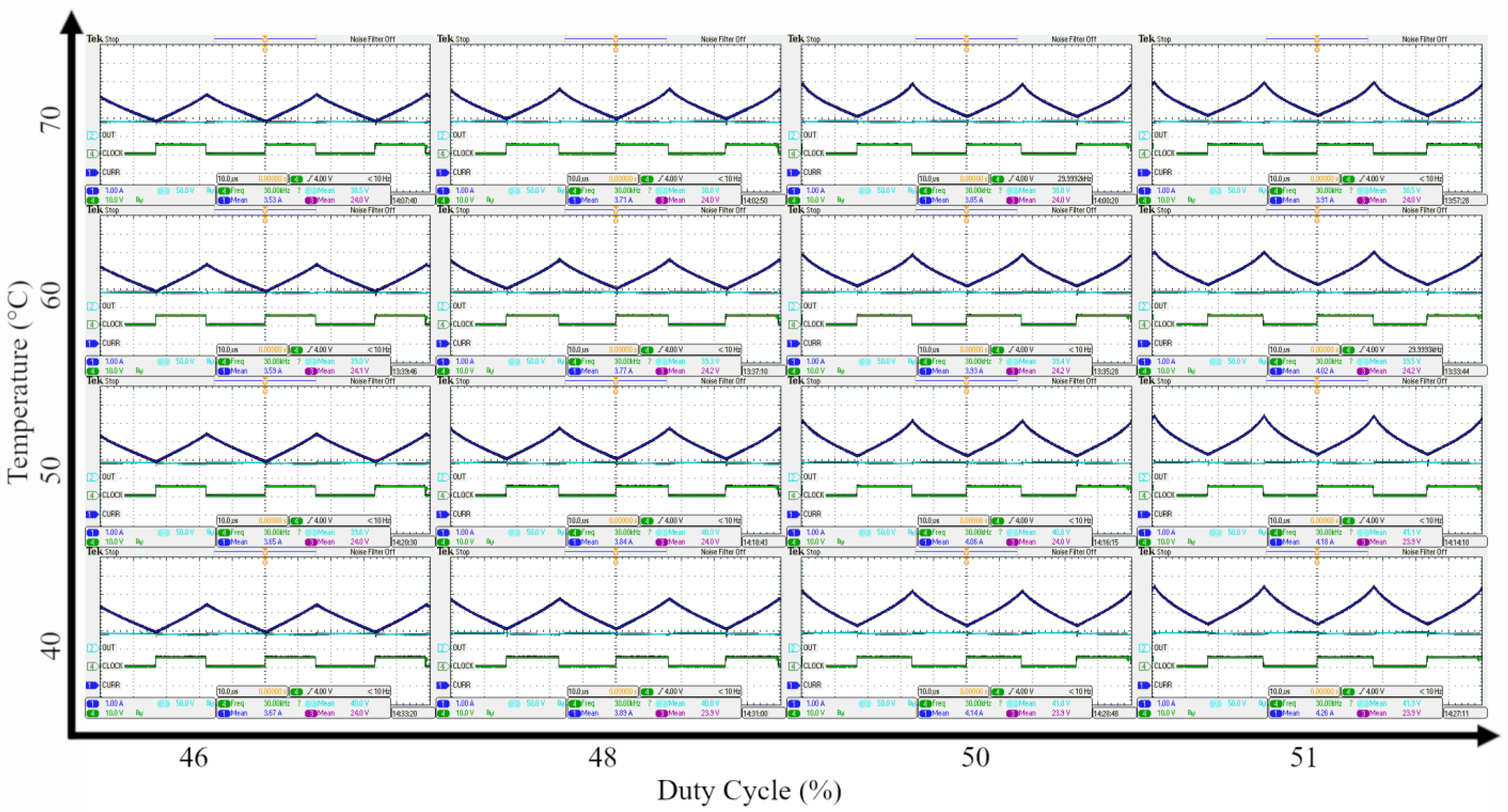
The experimental measurements are reported in Figure 6, each for a fixed core temperature and by varying the duty cycle. The value of the current peak for each measurement is reported in Table 2, highlighting its value when the temperature and duty cycle were changed. These measurements assess the influence of temperature on inductor operation and current profile. In fact, for a fixed temperature, an increase in the duty cycle, corresponding to an increase in the TON, leads to inductor operation outside the linear region. Moreover, the current profile depends on temperature. Because both the duty cycle and temperature can vary during the converter operation, this confirms the importance of using a tool for calculating the current profile. The results demonstrate that the proposed method can calculate the current profile under different working conditions up to its maximum value by exploiting the non-linearity of the inductor. Figure 6 is arranged for recognizing the effects of the temperature and of the conduction time on the maximum current value at a glance. Indeed, a rise in the maximum value can be appreciated by either increasing temperature or the duty cycle. Besides, the increase of the duty cycle (corresponding to an increase in the conduction time of the power switch) highlights the shape that no longer fits with a triangular waveform emphasizing the nonlinear behavior. The numerical values of the peaks are summarized in Table 2 where it can be noticed that the increase of the duty cycle induces an increase in the current peak that is more relevant for the highest temperature.
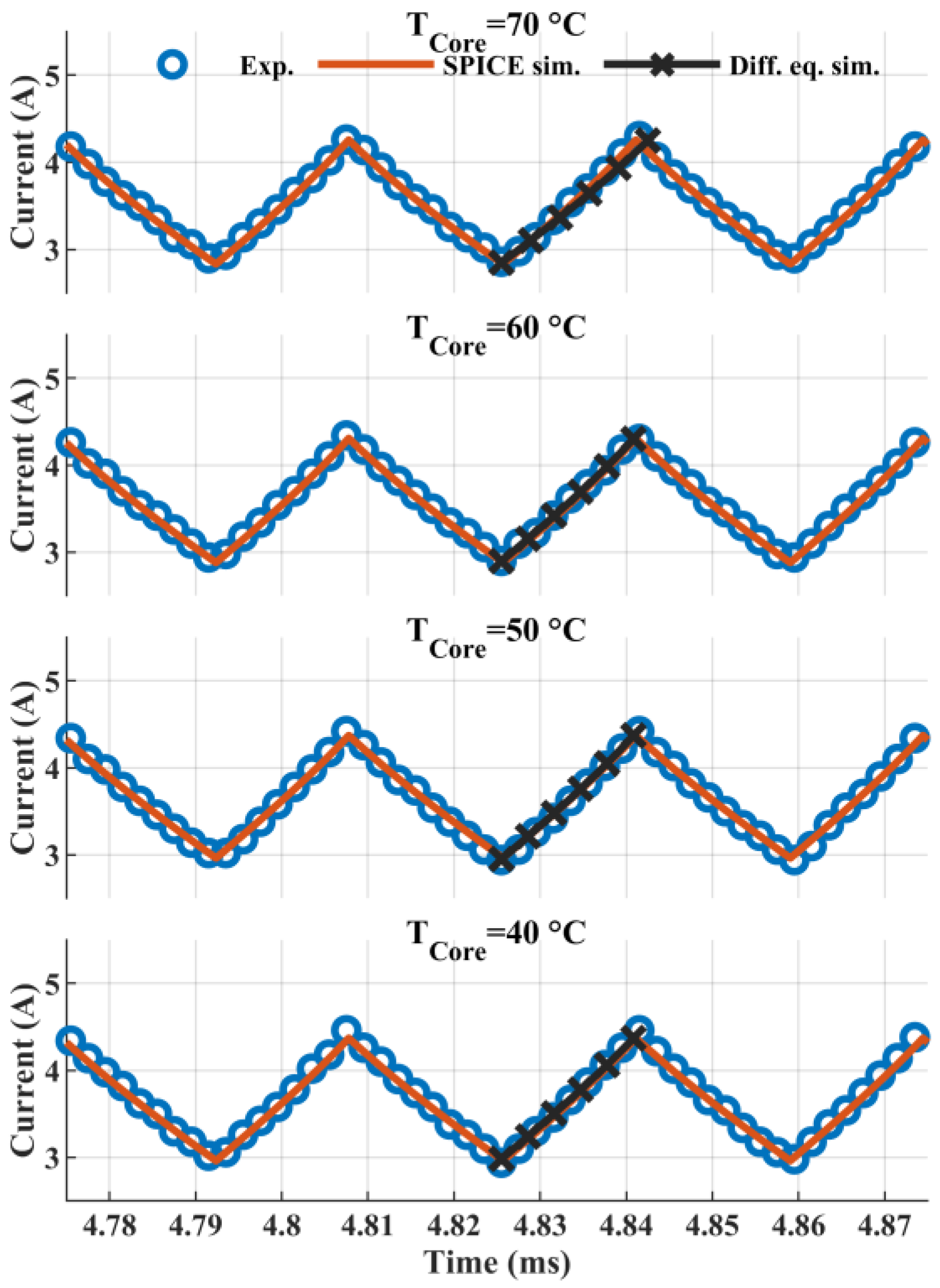
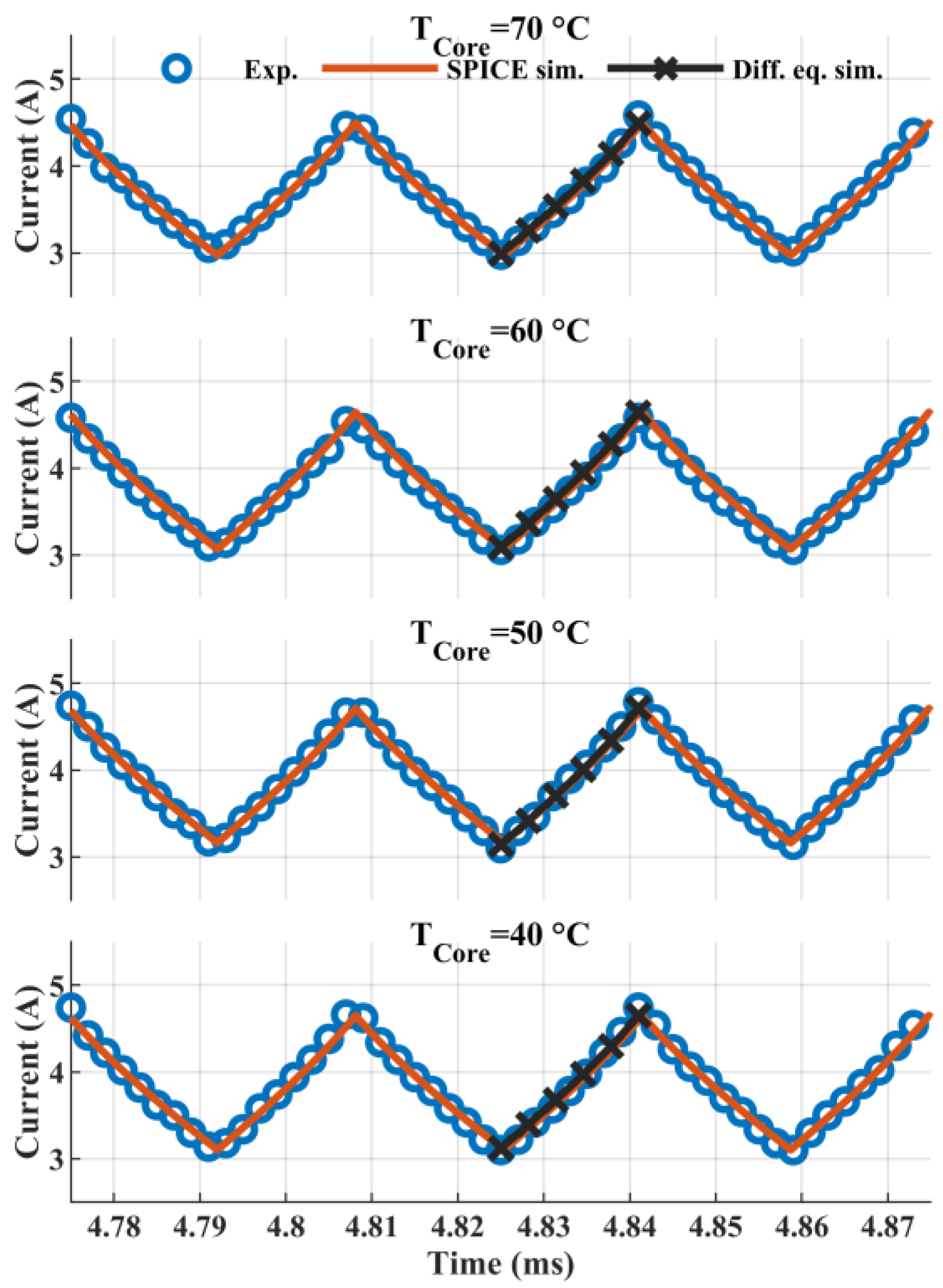
The simulations were carried out using LTspice software and solving the discrete differential Equation (4) using the polynomial curve and the previously described flux model to retrieve the current under the same conditions as the experimental test (Figure 6). The current curves calculated by solving Equation (3) through 4-th order Runge-Kutta were obtained in 104 steps. Figure 7, Figure 8, Figure 9 and Figure 10 compare the simulated and experimental data of the current waveform as a function of core temperature TCore for fixed duty cycles of 46, 48, 50, and 51%, respectively. By combining losses and inductor modeling, the relevant reduction in the peak current for increasing TCore, experimentally measured for each duty cycle, was correctly reproduced correctly. This effect is mainly due to the increased losses in the inductor due to the rising temperature.
The numerical values corresponding to the RMS current for cases with a duty cycle of 51% (representing the worst case) are listed in Table 3. In all cases, the relative error was below 9% for the SPICE simulations and below 3% for the discrete differential equation approach.
For validation purposes, the mean absolute error (MAE) was calculated by comparing the simulation results with the experimental data as a reference. Figure 11a compares the experimental data with those obtained by the simulations during the conduction period when the duty cycle was 51% and the temperature was set to 70 °C. Figure 11b shows the absolute error of each data point, resulting in an MAE of 94 mA for the SPICE simulations and 113 mA for the differential equation simulations. It should be noted that the minimum error was obtained at the end of the conduction time, meaning that both simulations tracked the current peak with excellent accuracy. All the comparisons highlight the excellent fit of the simulations with the experimental data. The MAE of each comparison of the experimental data with the SPICE simulation is given in Table 4 whereas the MAE regarding the differential equation is given in Table 5.
Figure 12 shows the spectra of the experimental currents, calculated by a Fast Fourier Transform (FFT), when the duty cycle was 50% and the core temperatures were 70 °C and 40 °C, respectively. As the temperature increases, the odd harmonics show a slight variation, which is negligible for the first harmonic at 30 kHz, whereas the even harmonics increase by more than 5 dB. The increase in the amplitude of the harmonics depends on the maximum value of the current through the inductor; as a consequence, the increase in the temperature worsens the EMI of the converter as well. The issues related to EMI filtering were discussed in [37,38], where, comparing the Fourier analysis performed on the same inductor in linear and non-linear operation, the increase of harmonics amplitude was shown. It required a re-design of the EMI filter, albeit the non-linear operation allowed an increase of the operating current of about 40% with related savings of cost and weight on the power inductor.
7. Conclusions
This paper is focused on applications of power electronics and computation for enhancing industrial systems and processes. Exploiting a power inductor up to saturation reduces the size of the magnetic core; however, this requires an assessment of the current to preserve the reliability of the converter.
A method was devised to retrieve the current profile in a power inductor operated up to saturation. The non-linear operation of an inductor modifies the shape of the current, which is no longer triangular as in the case of a linear inductor. This implies a higher peak, richer harmonic content, and non-linear dependence on conduction time and temperature. Therefore, knowing the current shape of the operating conditions is crucial to avoid dangerous situations for the devices in these SMPS and EMI evaluations.
The current profiles of an inductor up to saturation were estimated using a polynomial third-order inductor model in different operating conditions. This model was applied to a ferrite core inductor; however, it can reproduce the magnetization curve and be used for different core materials. The model also takes into account temperature. It has been used to both solve the constitutive equation of the inductor in discrete form and retrieve the flux model in closed form for implementation in a circuit simulator.
The current profile is obtained analytically and by simulation and completed with the analysis of the inductor current through experimental measurements and comparison with simulated results, including peak, RMS value, and spectrum evaluation. Furthermore, the quality of the simulations was evaluated through the mean absolute error of each comparison using the experimental result as a reference highlighting an adequate fit.
The operation of the inductor in saturation is of interest for industrial applications because it increases the converter’s maximum current, hence the power density, compared to a linear inductor. However, since the inductance changes with the current, very high peak values of the inductor current can be reached at the end of TON. The results showed that, based on a suitable inductor model, the proposed approach provides a complete assessment of the current, including the profile, its peak, RMS value, and spectrum. The analytical and simulation results agree with the experimental data measured using a boost converter. In addition, our analysis explains how the non-linear behavior of the inductor can be exploited when the duty cycle of an SMPS varies during operation.
The proposed approach can be generalized to any SMPS in which the inductor is subjected to a constant voltage for a given time interval. This aids in optimizing the converter design so that the non-linearity is exploited even with a variable duty cycle, while also considering the temperature.
The method proposed in this study allows designers to analyze the behavior of the SMPS starting from the maximum current of the non-linear inductor that can be chosen with a smaller core than a linear one improving the power density.
Author Contributions
Conceptualization, D.S., G.L. and G.V.; methodology, D.S., G.L. and G.V.; software, D.S., G.L. and G.V.; validation, D.S., G.L. and G.V.; formal analysis, D.S., G.L. and G.V.; investigation, D.S., G.L. and G.V.; resources, D.S., G.L. and G.V.; data curation, D.S., G.L. and G.V.; writing—original draft preparation, D.S., G.L. and G.V.; writing—review and editing, D.S., G.L. and G.V.; visualization, D.S., G.L. and G.V.; supervision, D.S., G.L. and G.V.; project administration, D.S., G.L. and G.V.; funding acquisition, D.S., G.L. and G.V. All authors have read and agreed to the published version of the manuscript.
Funding
This research was partially funded by the ECSEL-JU project REACTION (first and euRopEAn siC eigTh Inches pilOt liNe), Grant Agreement No. 783158.
Acknowledgments
The authors would like to thank Technician Giampiero Rizzo for the support in setting up the test bench and for helping with the experimental part.
Conflicts of Interest
The authors declare no conflict of interest.
References
- Di Capua, G.; Femia, N. A Novel Method to Predict the Real Operation of Ferrite Inductors with Moderate Saturation in Switching Power Supply Applications. IEEE Trans. Power Electron. 2016, 31, 2456–2464. [Google Scholar] [CrossRef]
- Perdigão, M.S.; Trovão, J.P.F.; Alonso, J.M.; Saraiva, E.S. Large-Signal Characterization of Power Inductors in EV Bidirectional DC-DC Converters Focused on Core Size Optimization. IEEE Trans. Ind. Electron. 2015, 62, 3042–3051. [Google Scholar] [CrossRef]
- Eichhorst, D.; Pfeiffer, J.; Zacharias, P. Weight Reduction of DC/DC Converters Using Controllable Inductors. In Proceedings of the PCIM Europe Conference Proceedings, Nuremberg, Germany, 7–9 May 2019; pp. 1670–1677. [Google Scholar]
- Martins, S.; Seidel, Á.R.; Perdigão, M.S.; Roggia, L. Core Volume Reduction Based on Non-Linear Inductors for a PV DC–DC Converter. Electr. Power Syst. Res. 2022, 213, 108716. [Google Scholar] [CrossRef]
- Sgrò, D.; Souza, S.A.; Tofoli, F.L.; Leão, R.P.S.; Sombra, A.K.R. An Integrated Design Approach of LCL Filters Based on Nonlinear Inductors for Grid-Connected Inverter Applications. Electr. Power Syst. Res. 2020, 186, 106389. [Google Scholar] [CrossRef]
- Abramovitz, A.; Ben-Yaakov, S.S. RGSE-Based SPICE Model of Ferrite Core Losses. IEEE Trans. Power Electron. 2018, 33, 2825–2831. [Google Scholar] [CrossRef]
- Bradley, E.; Kantz, H. Nonlinear Time-Series Analysis Revisited. Chaos 2015, 25, 097610. [Google Scholar] [CrossRef] [Green Version]
- Alzahrani, A.; Shamsi, P.; Ferdowsi, M.; Dagli, C. Chaotic Behavior of DC-DC Converters. In Proceedings of the 2017 6th International Conference on Renewable Energy Research and Applications, ICRERA 2017, San Diego, CA, USA, 5–8 November 2017. [Google Scholar]
- Valchev, V.C.; van den Bossche, A. Inductors and Transformers for Power Electronics, 1st ed.; CRC Press: Boca Raton, FL, USA, 2018; ISBN 9781315221014. [Google Scholar]
- Vitale, G.; Lullo, G.; Scire, D. Thermal Stability of a DC/DC Converter with Inductor in Partial Saturation. IEEE Trans. Ind. Electron. 2021, 68, 7985–7995. [Google Scholar] [CrossRef]
- Liu, B.; Chen, W.; Wang, J.; Chen, Q. A Practical Inductor Loss Testing Scheme and Device with High Frequency Pulsewidth Modulation Excitations. IEEE Trans. Ind. Electron. 2021, 68, 4457–4467. [Google Scholar] [CrossRef]
- Musumeci, S.; Solimene, L.; Ragusa, C.S. Identification of DC Thermal Steady-State Differential Inductance of Ferrite Power Inductors. Energies 2021, 14, 3854. [Google Scholar] [CrossRef]
- Detka, K.; Górecki, K. Electrothermal Model of Coupled Inductors with Nanocrystalline Cores. Energies 2022, 15, 224. [Google Scholar] [CrossRef]
- Scirè, D.; Vitale, G.; Ventimiglia, M.; Lullo, G. Non-Linear Inductors Characterization in Real Operating Conditions for Power Density Optimization in SMPS. Energies 2021, 14, 3924. [Google Scholar] [CrossRef]
- Sferlazza, A.; Albea-Sanchez, C.; Garcia, G. A Hybrid Control Strategy for Quadratic Boost Converters with Inductor Currents Estimation. Control Eng. Pract. 2020, 103, 104602. [Google Scholar] [CrossRef]
- Hassani, V.; Tjahjowidodo, T.; Do, T.N. A Survey on Hysteresis Modeling, Identification and Control. Mech. Syst. Signal Process. 2014, 49, 209–233. [Google Scholar] [CrossRef]
- Kosai, H.; Turgut, Z.; Scofield, J. Experimental Investigation of DC-Bias Related Core Losses in a Boost Inductor. IEEE Trans. Magn. 2013, 49, 4168–4171. [Google Scholar] [CrossRef]
- Matsumori, H.; Shimizu, T.; Wang, X.; Blaabjerg, F. A Practical Core Loss Model for Filter Inductors of Power Electronic Converters. IEEE J. Emerg. Sel. Top. Power Electron. 2018, 6, 29–39. [Google Scholar] [CrossRef]
- Nakano, S.; Nakazawa, T.; Matsumoto, Y.; Otsuki, E. Power Loss Analysis of SMD Power Inductors. In Proceedings of the Conference Proceedings—IEEE Applied Power Electronics Conference and Exposition—APEC, Fort Worth, TX, USA, 6–11 March 2011; pp. 1687–1691. [Google Scholar]
- Górecki, K.; Detka, K. Application of Average Electrothermal Models in the SPICE-Aided Analysis of Boost Converters. IEEE Trans. Ind. Electron. 2019, 66, 2746–2755. [Google Scholar] [CrossRef]
- Górecki, K.; Godlewska, M. Elektrotermiczny Model Rdzenia Ferromagnetycznego. Prz. Elektrotech. 2015, 91, 161–165. [Google Scholar] [CrossRef]
- Bizzarri, F.; Lodi, M.; Oliveri, A.; Brambilla, A.; Storace, M. A Nonlinear Inductance Model Able to Reproduce Thermal Transient in SMPS Simulations. In Proceedings of the—IEEE International Symposium on Circuits and Systems, Sapporo, Japan, 26–29 May 2019; pp. 1–5. [Google Scholar]
- Lodi, M.; Oliveri, A.; Storace, M. Behavioral Models for Ferrite-Core Inductors in Switch-Mode DC-DC Power Supplies: A Survey. In Proceedings of the 5th International Forum on Research and Technologies for Society and Industry: Innovation to Shape the Future, RTSI 2019—Proceedings, Florence, Italy, 9–12 September 2019; pp. 242–247. [Google Scholar] [CrossRef]
- Scirè, D.; Lullo, G.; Vitale, G. Non-Linear Inductor Models Comparison for Switched Mode-Power Supplies Applications. Electronics 2022, 11, 2472. [Google Scholar] [CrossRef]
- Oliveri, A.; Lodi, M.; Storace, M. Nonlinear Models of Power Inductors: A Survey. Int. J. Circuit Theory Appl. 2022, 50, 2–34. [Google Scholar] [CrossRef]
- Burrascano, P.; di Capua, G.; Laureti, S.; Ricci, M. Neural Models of Ferrite Inductors Non-Linear Behavior. In Proceedings of the Proceedings—IEEE International Symposium on Circuits and Systems, Sapporo, Japan, 26–29 May 2019. [Google Scholar]
- Oliveri, A.; Lodi, M.; Storace, M. A Piecewise-Affine Inductance Model for Inductors Working in Nonlinear Region. In Proceedings of the SMACD 2019—16th International Conference on Synthesis, Modeling, Analysis and Simulation Methods and Applications to Circuit Design, Proceedings, Lausanne, Switzerland, 15–18 July 2019; pp. 169–172. [Google Scholar]
- Oliveri, A.; di Capua, G.; Stoyka, K.; Lodi, M.; Storace, M.; Femia, N. A Power-Loss-Dependent Inductance Model for Ferrite-Core Power Inductors in Switch-Mode Power Supplies. IEEE Trans. Circuits Syst. I Regul. Pap. 2019, 66, 2394–2402. [Google Scholar] [CrossRef]
- Barili, A.; Brambilla, A.; Cottafava, G.; Dallago, E. A Simulation Model for the Saturable Reactor. IEEE Trans. Ind. Electron. 1988, 35, 301–306. [Google Scholar] [CrossRef]
- Raggl, K.; Nussbaumer, T.; Kolar, J.W. Guideline for a Simplified Differential-Mode EMI Filter Design. IEEE Trans. Ind. Electron. 2010, 57, 1031–1040. [Google Scholar] [CrossRef]
- McLyman, C.W.T. Transformer and Inductor Design Handbook, 4th ed.; CRC Press: Boca Raton, FL, USA, 2017; ISBN 9781315217666. [Google Scholar]
- Kachniarz, M.; Salach, J.; Szewczyk, R.; Bieńkowski, A. Temperature Influence on the Magnetic Characteristics of Mn-Zn Ferrite Materials. In Progress in Automation, Robotics and Measuring Techniques; Advances in Intelligent Systems and Computing; Szewczyk, R., Zieliński, C., Kaliczyńska, M., Eds.; Springer International Publishing: Cham, Switzerland, 2015; Volume 352, pp. 121–127. [Google Scholar]
- Lu, H.Y.; Zhu, J.G.; Hui, S.Y.R. Measurement and Modeling of Thermal Effects on Magnetic Hysteresis of Soft Ferrites. IEEE Trans. Magn. 2007, 43, 3952–3960. [Google Scholar] [CrossRef]
- Nichols, K.G.; Kazmierski, T.J.; Zwolinski, M.; Brown, A.D. Overview of SPICE-like Circuit Simulation Algorithms. IEE Proc. Circuits Devices Syst. 1994, 141, 242–250. [Google Scholar] [CrossRef]
- Butusov, D.; Karimov, A.; Tutueva, A.; Kaplun, D.; Nepomuceno, E.G. The Effects of Padé Numerical Integration in Simulation of Conservative Chaotic Systems. Entropy 2019, 21, 362. [Google Scholar] [CrossRef] [Green Version]
- Zhou, X.; Li, J.; Ma, Y. Chaos Phenomena in DC-DC Converter and Chaos Control. Procedia Eng. 2012, 29, 470–473. [Google Scholar] [CrossRef] [Green Version]
- Scire, D.; Lullo, G.; Vitale, G. EMI Filter Re-Design in a SMPS with Inductor in Saturation. In Proceedings of the 2021 IEEE 15th International Conference on Compatibility, Power Electronics and Power Engineering (CPE-POWERENG), Florence, Italy, 14–16 July 2021; pp. 1–7. [Google Scholar]
- Scirè, D.; Lullo, G.; Vitale, G. EMI Worsening in a SMPS with Non-Linear Inductor. Renew. Energy Power Qual. J. 2022, 20, 512–519. [Google Scholar] [CrossRef]
Figure 1.
Boost converter representation.

Figure 2.
Comparison of current waveforms with linear and non-linear inductors.

Figure 3.
Comparison of experimental points obtained from inductor characterization with model (1).

Figure 4.
(a) Photo of the test rig. (b) pictorial diagram of the test rig.

Figure 5.
An oscilloscope plot of the current flowing through the power switch shows the influence of TON on saturation: (a) a linear trend is observed for TON = 15 µs, and (b) a non-linear trend for TON = 17 µs.
Figure 5.
An oscilloscope plot of the current flowing through the power switch shows the influence of TON on saturation: (a) a linear trend is observed for TON = 15 µs, and (b) a non-linear trend for TON = 17 µs.

Figure 6.
Oscilloscope plots of the current flowing through the inductor (blue), output voltage (cyan), and gate voltage (green) for increasing duty cycle ratio and temperature at a switching frequency of 30 kHz.
Figure 6.
Oscilloscope plots of the current flowing through the inductor (blue), output voltage (cyan), and gate voltage (green) for increasing duty cycle ratio and temperature at a switching frequency of 30 kHz.

Figure 7.
Comparison of the experimental current waveform with the simulation results from SPICE and the differential equation for a duty cycle of 46% at different temperatures.
Figure 7.
Comparison of the experimental current waveform with the simulation results from SPICE and the differential equation for a duty cycle of 46% at different temperatures.

Figure 8.
Comparison of the experimental current waveform with the simulation results from SPICE and the differential equation for a duty cycle of 48% at different temperatures.
Figure 8.
Comparison of the experimental current waveform with the simulation results from SPICE and the differential equation for a duty cycle of 48% at different temperatures.

Figure 9.
Comparison of the experimental current waveform with the simulation results from SPICE and the differential equation for a duty cycle of 50% at different temperatures.
Figure 9.
Comparison of the experimental current waveform with the simulation results from SPICE and the differential equation for a duty cycle of 50% at different temperatures.

Figure 10.
Comparison of the experimental current waveform with the simulation results from SPICE and the differential equation for a duty cycle of 51% at different temperatures.
Figure 10.
Comparison of the experimental current waveform with the simulation results from SPICE and the differential equation for a duty cycle of 51% at different temperatures.

Figure 11.
(a) Comparison of the experimental current waveform with the simulation results from SPICE and differential equation for a duty cycle of 51% at 70 °C. (b) Comparison of mean absolute error for SPICE and differential equation simulations.
Figure 11.
(a) Comparison of the experimental current waveform with the simulation results from SPICE and differential equation for a duty cycle of 51% at 70 °C. (b) Comparison of mean absolute error for SPICE and differential equation simulations.

Figure 12.
FFT AC spectra of experimental inductor current for a duty cycle of 50% at different temperatures.
Figure 12.
FFT AC spectra of experimental inductor current for a duty cycle of 50% at different temperatures.


Table 1.
Model coefficients of the inductor.
| Coefficient | Value | Coefficient | Value (1/°C) |
|---|---|---|---|
| L0 | 262 × 10−6 | β0 | −0.0006 |
| L1 | −28.8 × 10⁻⁶ | β1 | −0.0240 |
| L2 | 22.9 × 10⁻⁶ | β2 | −0.0150 |
| L3 | −3.72 × 10⁻⁶ | β3 | −0.0090 |
| Ldeepsat | 50 × 10−6 |
Table 2.
Inductor current peak (in A) for different duty cycles and temperatures.
| (A) | Temperature | |||
|---|---|---|---|---|
| Duty Cycle | 40 °C | 50 °C | 60 °C | 70 °C |
| 46% | 4.26 | 4.31 | 4.37 | 4.37 |
| 48% | 4.50 | 4.64 | 4.71 | 4.65 |
| 50% | 4.76 | 4.93 | 5.06 | 5.12 |
| 51% | 4.98 | 5.00 | 5.31 | 5.39 |
Table 3.
RMS current (in A) comparison when the duty cycle is 51%.
| Temperature (°C) | Duty Cycle (%) | Experimental (A) | SPICE Simulation (A) | Differential Equation Simulation (A) |
|---|---|---|---|---|
| 70 | 51 | 3.94 | 4.28 (+8.6%) | 4.06 (+3.0%) |
| 60 | 51 | 4.05 | 4.22 (+4.2%) | 4.10 (+1.2%) |
| 50 | 51 | 4.22 | 4.45 (+5.5%) | 4.30 (+1.9%) |
| 40 | 51 | 4.30 | 4.51 (+4.9%) | 4.37 (+1.6%) |
Table 4.
Mean absolute error (in mA) of the inductor current for different duty cycles and temperatures for the SPICE simulations.
Table 4.
Mean absolute error (in mA) of the inductor current for different duty cycles and temperatures for the SPICE simulations.
| (mA) | Temperature | |||
|---|---|---|---|---|
| Duty Cycle | 40 °C | 50 °C | 60 °C | 70 °C |
| 46% | 45.8 | 30.3 | 44.9 | 40.5 |
| 48% | 31.2 | 26.1 | 24.4 | 29.8 |
| 50% | 92 | 38.9 | 53.4 | 27.4 |
| 51% | 59.7 | 85.6 | 55.5 | 94.6 |
Table 5.
Mean absolute error (in mA) of the inductor current for different duty cycles and temperatures for the differential equation simulations.
Table 5.
Mean absolute error (in mA) of the inductor current for different duty cycles and temperatures for the differential equation simulations.
| (mA) | Temperature | |||
|---|---|---|---|---|
| Duty Cycle | 40 °C | 50 °C | 60 °C | 70 °C |
| 46% | 36.4 | 33.3 | 37.6 | 97.9 |
| 48% | 25.4 | 33.2 | 34.2 | 21.6 |
| 50% | 46.6 | 51.2 | 68.2 | 37.4 |
| 51% | 73.2 | 83.1 | 35.1 | 113.4 |
Disclaimer/Publisher’s Note: The statements, opinions and data contained in all publications are solely those of the individual author(s) and contributor(s) and not of MDPI and/or the editor(s). MDPI and/or the editor(s) disclaim responsibility for any injury to people or property resulting from any ideas, methods, instructions or products referred to in the content. |
© 2023 by the authors. Licensee MDPI, Basel, Switzerland. This article is an open access article distributed under the terms and conditions of the Creative Commons Attribution (CC BY) license (https://creativecommons.org/licenses/by/4.0/).
Share and Cite
MDPI and ACS Style
Scirè, D.; Lullo, G.; Vitale, G. Assessment of the Current for a Non-Linear Power Inductor Including Temperature in DC-DC Converters. Electronics 2023, 12, 579. https://0-doi-org.brum.beds.ac.uk/10.3390/electronics12030579
AMA Style
Scirè D, Lullo G, Vitale G. Assessment of the Current for a Non-Linear Power Inductor Including Temperature in DC-DC Converters. Electronics. 2023; 12(3):579. https://0-doi-org.brum.beds.ac.uk/10.3390/electronics12030579
Chicago/Turabian StyleScirè, Daniele, Giuseppe Lullo, and Gianpaolo Vitale. 2023. "Assessment of the Current for a Non-Linear Power Inductor Including Temperature in DC-DC Converters" Electronics 12, no. 3: 579. https://0-doi-org.brum.beds.ac.uk/10.3390/electronics12030579
Note that from the first issue of 2016, this journal uses article numbers instead of page numbers. See further details here.