Siamese Neural Pointnet: 3D Face Verification under Pose Interference and Partial Occlusion

Abstract

Face verification based on ordinary 2D RGB images has been widely used in daily life. However, the quality of ordinary 2D RGB images is limited by illumination, and they lack stereoscopic features, which makes it difficult to apply them in poor lighting conditions and means they are susceptible to interference from head pose and partial occlusions. Considering point clouds are not affected by illumination and can easily represent geometric information, this paper constructs a novel Siamese network for 3D face verification based on Pointnet. In order to reduce the influence of the self-generated point clouds, the chamfer distance is adopted to constrain the original point clouds and explore a new energy function to distinguish features. The experimental results with the Pandora and Curtin Faces datasets show that the accuracy of the proposed method is improved by 0.6% compared with the latest methods; in large pose interference and partial occlusion, the accuracy is improved by 4% and 5%. The results verify that our method outperforms the latest methods and can be applied to a variety of complex scenarios while maintaining real-time performance.

1. Introduction

Face recognition algorithms are traditionally split into two specific tasks by the computer vision community: verification and identification [1]. Different from face identification, face verification is a one-to-one comparison task; given a pair of images as input, a face verification system should predict if the input items contain faces of the same person or not [2]. The computer vision community has broadly addressed the problem in both the 2D RGB and 3D domains [3]. However, ordinary RGB cameras cannot obtain effective images in the case of a large variation of illumination. In addition, 2D RGB images lack stereo information and are more susceptible to interference from head pose and partial occlusion.

Recently, the computation of geometric descriptors of 3D shapes has played an important role in many 3D computer vision applications [4]. In general, 3D objects are mainly represented by the following four methods: mesh, voxel grid, octree, and point cloud. However, the expression of mesh is complex, the voxel grid makes the space redundant, and the octree is complicated to use. In contrast, the point cloud can be directly used to represent 3D information, and the mathematical expression is very concise. With the improvement of depth map devices, obtaining effective point clouds has become easier. Depth maps have two main advantages. Firstly, the devices are stable with illumination changes. Secondly, depth maps can be easily exploited to manage the scale of the target object in detection tasks [5]. However, compared with point clouds, depth maps have two disadvantages. First, depth maps are expressed in the form of single-channel 2D images, which cannot directly reflect the geometric characteristics of objects in a 3D space. Second, the contours of depth maps overlap with the surrounding pixels, which makes the contours unclear, and some important information will be lost. Relying on a simple coordinate transformation, depth maps can be converted into point clouds; therefore, point clouds inherit the above two advantages of depth maps and also keep clearer geometric characteristics. Furthermore, since the pioneering work of Charles et al. [6], who constructed Pointnet, which solves the sparsity and disorder of point clouds, many deep learning models have been proposed, and point clouds now have more abundant applications.

In this paper, in order to reduce interference from head pose and partial occlusion, we rely on point clouds to construct a novel Siamese network for 3D face verification. In our method, we first obtain face information from depth maps and convert it to point clouds. Secondly, we construct a Siamese network to extract features. In this step, we adopt the farthest point sampling algorithm to sample points and employ two set abstractions to extract local-to-global face features hierarchically. Thirdly, in order to reduce the influence of the self-generated point clouds, we employ the chamfer distance to constrain the original point clouds and design a new energy function to measure the difference between two features.

In order to verify the performance of our method, we conduct experiments on two public datasets—the Pandora dataset and the Curtin Faces dataset. We also split the Pandora dataset into groups for cross-training and testing to verify the effectiveness of our method under pose interference and partial occlusion.

The main contributions of this paper are summarized as follows:

• We propose an end-to-end 3D face verification network, which, to the best of our knowledge, is the first attempt to construct a Siamese network with point clouds for face verification.
• We employ the charm distance to constrain the original point clouds, which can effectively improve the accuracy, and enables our network to better cope with the interference from head pose and partial occlusion.
• The experimental results on public datasets show that our network has good real-time performance, and the verification accuracy outperforms the latest methods, especially under pose interference and partial occlusion.

2. Related Works

In recent years, the most widely used face verification methods have mainly been based on intensity images [7]. Before neural networks became widely used for image tasks, most of the methods were based on hand-crafted features [8]. With the improvement of hardware such as GPUs, more deep learning methods in neural networks have been applied to computer vision. Benefiting from the perceptual power of deep learning, most methods outperform humans on the LFW dataset [9]. Among them, Schroff et al. [10] constructed a network, FaceNet, which takes pairs of images as inputs and introduces a triplet loss to calculate the difference between images. In [11], Phillips et al. designed a VGG-face algorithm to recognize faces as variables. Richardson et al. [12] combined CoarseNet and FineNet and introduced an end-to-end CNN framework that derives the shape in a coarse-to-fine fashion. In order to avoid noise and degradation, Deng et al. [13] explored a robust binary face descriptor, compressive binary patterns (CBP). Wu et al. [14] proposed a center invariant loss and added a penalty to the differences between each center of classes to generate a robust and discriminative face representation method. Wang et al. [15] introduced a more interpretable additive angular margin for the softmax loss in face verification and discussed the importance of feature normalization. To combat the data imbalance, Ding et al. [16] combined generative adversarial networks and a classifier network to construct a one-shot face recognition network. Likewise, in order to deal with the imbalance problem, based on margin-aware reinforcement learning, Liu et al. [17] introduced a fair loss, in which deep Q-learning is used to learn an appropriate adaptive margin for each class. Targeting racial and gender differences in face recognition, Zhu et al. [18] combined NAS technology and the reinforcement learning strategy into a face recognition task and proposed a novel deep neural architecture search network. In order to deal with low-resolution face verification, Jiao et al. [19] constructed an end-to-end low-resolution face translation and verification framework which improves the accuracy of face verification while improving the quality of face images. Recently, Lin et al. [20] proposed a novel similarity metric, called explainable cosine, which can be plugged into most of the verification models to provide meaningful explanations. Aimed at facial comparison in a forensic context, Verma et al. [21] employed an automatic approach to detect facial landmarks, and selected independent facial indices extracted from a subset of these landmarks. Cao et al. [22] introduced two descriptors and one composite operator to construct a framework named GMLM-CNN for face verification between short-wave infrared and visible light.

Compared to RGB images, depth maps lack texture detail, but they cope well with dramatic light changes. Based on the depth maps, Guido et al. [23] generated other types of pictures using a GAN network for head pose estimation. In [7,24], Ballota et al. utilized convolutional neural networks for head detection, marking the first time CNN was leveraged for head detection based on depth images. In recent years, many face verification methods based on depth maps have been proposed. Borghi et al. [3] constructed JanusNet, which is a hybrid Siamese network composed of depth and RGB images. Subsequently, Borghi et al. [2] used two fully convolutional networks to build a Siamese network, which only relies on deep images for training and testing and achieved very good results. Afterwards, Wang et al. [25] adopted a one-shot Siamese network for depth face verification which significantly improved the accuracy. In order to reduce the interference from the head pose, Zou et al. [26] projected the face features onto a 2D plane and introduced the attention mechanism to reduce interference from facial expressions. Rajagopal et al. [27] introduced a CDS feature vector and proposed three levels of networks for face expression categorization. Wang et al. [28] used L2 to constrain facial features and constructed an L2–Siamese network for depth face verification.

Most of the proposed related 3D methods have achieved excellent performance. In order to solve the photometric stereo for non-Lambertian surfaces and a disordered and arbitrary number of input features, Chen et al. [29] proposed a deep fully convolutional network PS-FCN to predict a normal map of the object in a fast feed-forward pass. Aiming at 3D geometry reconstruction and avoiding blurred reconstruction, Ju et al. [30] proposed a self-learning conditional network with multi-scale features for photometric stereo. Similar to depth maps, surface normal maps can also provide 3D information for relevant tasks. The pioneers Woodham et al. [31] proposed photometric stereo, which varies the direction of incident illumination between successive images while holding the viewing direction constant to recover the surface normal of each of the image points. Recently, Ju et al. [32] presented a normalized attention-weighted photometric stereo network NormAttention-PSN, which significantly improved surface orientation prediction for complicated structures.

In the field of 3D point cloud vision, building on the innovation of Pointnet, Qi et al. [6] solved the disorder and application in deep learning of point clouds; although many point cloud methods are proposed, this work only considered the global features and missed local features. Subsequently, Charles et al. [33] improved Pointnet by extracting local features from a group of Pointnets. In order to solve the application of point clouds in convolutional neural networks, Li et al. [34] proposed Pointcnn to learn X-transformation, which is the generalization of typical CNNs into learning features. Guerrero et al. [35] changed the first transformation of Pointnet and proposed PCPNet, which avoids the quality defects of the point clouds and reduces the interference of invalid points. The above works [33,34,35] optimize the feature extraction of point clouds and maintain good real-time performance, but they did not consider the spatial geometric characteristics of original points. In PPFNet, Deng et al. [36] applied a four-dimensional feature descriptor to describe the geometric characteristics of original point pairs. Zhou et al. [4] constructed a Siamese point network for feature extraction and measured the difference between the original point clouds. Both [4] and [36] considered the spatial geometric characteristics of the original point clouds, but they adopted a matrix for registration, which is computationally intensive and time-consuming.

As mentioned above, many point-cloud-based networks have been proposed, and they have their own advantages. Due to these advantages, many face analysis methods are proposed. Recently, Xiao et al. [37] constructed a classification network to guide the regression process of Pointnet++ for head pose estimation. Ma et al. [38] combined a deep regression forest and Pointnet for predicting head pose. Cao et al. [39] proposed a local descriptor to describe the projection of point clouds for 3D face recognition.

Face verification is a one-to-one comparison task taking into account both the effectiveness of feature extraction and real-time performance. Based on Pointnet, we construct a novel Siamese network and adopt the chamfer distance to constrain the geometric characteristics of the original point clouds.

3. Methods

For face verification with 3D point clouds, we convert the depth maps into point clouds, construct a Siamese network to extract the features of a pair of faces, and employ the chamfer distance to design the energy function to predict the similarity between the two faces.

3.1. Point Cloud Extraction

As described above, we transform depth maps to point clouds. This means converting depth data from an image coordinate system to the world coordinate system. Each pixel of a depth map represents the distance from the target to the sensor (in mm). In this step, we assume that the whole head information and head center $(x^{\text{'}},y^{\text{'}})$ with its depth value $D_p$ has been obtained (head detection and center localization are not the focus of our work). Firstly, removing the background, we set the pixel value, which is greater than $D_p$ + L to 0, where L is the general amount of space for a real head [24] (300 mm in our method). Secondly, according to Equation (1), we convert depth data to point clouds.

$$\left[\begin{array}{c}x\\ y\\ z\end{array}\right]=D_p\left[\begin{array}{ccc}\frac{1}{f_x}& 0& 0\\ 0& \frac{1}{f_y}& 0\\ 0& 0& 1\end{array}\right]\left[\begin{array}{c}{x}^i\\ y^i\\ 1\end{array}\right]$$

(1)

where (x, y, z) is the point location in the world coordinate system, and $(x^i,y^i)$ is the pixel position in the image. $f_x$ and $f_y$ are camera internal parameters which represent the horizontal and the vertical focal length, respectively. As shown in Equation (1), a point cloud is a list of points (represent in position (x, y, z)) in a 3D space.

3.2. Siamese Neural Network

Siamese neural networks were first proposed and applied to the signature and verification certificate tasks by Bromley et al. [40]. A Siamese network consists of two shared weight networks which accept distinct inputs and are joined by an energy function at the end. This energy function computes a metric between two high-level features. The parameters between the twin networks are tied, which can guarantee network consistency, and ensures that a pair of very similar features are not mapped to very different locations in feature space by the respective networks [41].

The structure of the Siamese neural network is shown in Figure 1. The input layer sends an object to the hidden layer which extracts object features. The ends of two networks are connected by an energy function in the distance layer which computes certain metrics between features based on task requirements. Output layers predict the result of the Siamese network.

3.3. Feature Extraction

As mentioned above, the essence of a point cloud is a list of points ($n\times 3$ matrix, where n is the number of points, and 3 represents (x, y, z) in the world coordinates). Geometrically, the order of points does not affect its representation of the overall shape in 3D space. As shown in Figure 2, the same point clouds can be represented by completely different matrices. In order to deal with the disorder of point clouds and their application in deep learning, Chen et al. [6], based on the idea of symmetric function, constructed a deep learning model called Pointnet. The idea is to approximate a general function by applying a symmetric function:

$$f(x_1,x_2,x_3,\cdots ,x_n)\approx \gamma \circ g(h(x_1),h(x_2),h(x_3),\cdots ,h(x_n))$$

(2)

where f is a general function, which maps all independent variables $(x_1,x_2,x_{3,}\cdots ,x_n)$ to a new feature space ${ℝ}^m$. h is another general function used to map each independent variable $x_i$ to feature space ${ℝ}^l$, and g is a symmetric function (the input order does not affect the result). r is also a general function which maps the result of function g to the specific feature space ${ℝ}^m$. According to Equation (2), the left part of the equation can be approximated by the right part. As described above, we adopt Pointnet to approximate the right part.

The structure of the network is shown in Figure 3.

As shown in Figure 3, where n is the total number of points. We adopt three convolutional layers as the function h in Equation (2) (convolution kernel is $1\times 1$, the filter is k, l, m, respectively), which is used to map the feature of each point to the feature space ${ℝ}^3\to {ℝ}^k\to {ℝ}^l\to {ℝ}^m$. Finally, according to [6,29,30], a max pooling layer is adopted as the symmetric function, g, which can solve the disorder of the features and extract the global feature in ${ℝ}^m$.

As described above, only the global feature of the object can be obtained by Pointnet. There is no step to extract local features. Because point clouds lack a detailed texture, only global features lead to a limited generalization ability of the network, especially in complex scenarios. In order to improve the cognitive ability of the network, according to [33], we adopt the set abstraction to extract the local-to-global features. The structure of a set abstraction is shown in Figure 4. A set abstraction consists of the following three parts: sampling, grouping, and local feature extraction. For a point cloud $\{p_1,p_2,p_3,\dots ,p_N\}$(the feature dimension of these points is C), in order to sample uniformly, we first use the farthest point sampling method to sample the points. In this step, we arbitrarily select a point $p_i$ as the starting point and find the farthest point $p_{i1}$ from the point cloud, and put $p_{i1}$ into a new point set. Next, we regard $p_{i1}$ as a new starting point and find the farthest point in the rest of the points. We iterate the above steps until we obtain a new point set $\{p_{11},p_{12},p_{13},\dots ,p_{1N_1}\}$ with a fixed number $N_1$. Compared with random sampling, farthest point sampling can cover the whole point set [42].

Secondly, we group these points in $\{p_{11},p_{12},p_{13},\dots ,p_{1N_1}\}$; in this step, we regard each point as the center of a sphere with radius K (our network contains two set abstractions with a K of 0.2 and 0.4, respectively), and points in the same sphere are grouped into one group. After this step, we obtain a new grouping set $\{g_1,g_2,g_3,\cdots ,g_{N_1}\}$, and each group represents a local region of its own central point.

Finally, we use a Pointnet, as shown in Figure 3, to extract features of each group, and obtain a set of local features $\{f_1,f_2,f_3,\dots ,f_{N_1}\}$(the dimension of these features is $C_1$). We regard $\{f_1,f_2,f_3,\dots ,f_{N_1}\}$ as a new point set for the abstraction of the next step.

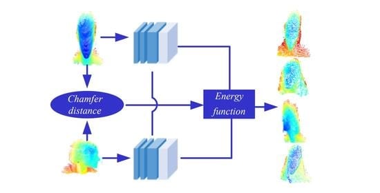
The process of our method is shown in Figure 5, and we use a pair of completely parallel branches to extract head features separately. Each branch contains two set abstractions. The first set abstraction adopts Pointnet1 to extract local features, which has three convolutional layers, and the filter of each layer is 64, 64, 128, respectively. The second set abstraction adopts Pointnet2 to extract local features, which also has three convolutional layers, and the filter of each layer is 128, 128, 256, respectively. After the second set abstraction, each branch employs Pointnet3 (The filters of three convolutional layers are 256, 512, 1024) to extract the local-to-global features of the object.

In practice, although the furthest point sampling method samples uniformly, due to the unevenness of the point cloud, some groups have fewer points. During the grouping process, the density and sparseness of points will affect the feature extraction. Therefore, we use multi-resolution grouping to obtain the features of each layer.

As shown in Figure 6, the features of a set abstraction are composed of two vectors. The left vector is the features of each group in this set abstraction. The right vector is the features of the original points of the previous layer for groups with sparse points which makes the first vector less reliable. Therefore, the second vector learns a higher weight during training. On the other hand, for groups with dense points, the networks obtain finer feature information, and the first vector learns a higher weight. In the training process, the network adjusts the weights in the above way to find the optimal weights for different point densities [42].

3.4. Feature Constraint

Siamese networks measure the difference between high-dimensional features but lack a description of the difference between original point clouds. The chamfer distance can represent the original differences of point clouds and is widely used in point cloud reconstruction [4]. In order to reduce the influence of the self-generated point clouds, we adopt chamfer distance (CD) to constrain their features. It is defined as follows:

$$d_{CD}(S_1,S_2)={\displaystyle \sum _{p\in S_1}\underset{q\in S_2}{\min }d(p,q)}+{\displaystyle \sum _{p\in S_2}\underset{q\in S_1}{\min }d(p,q)}$$

(3)

where $S_1,S_2\in {ℝ}^3$ represent two sets of point clouds. $d(p,q)$ measures the L2 distance between points p and q. The first term represents the sum of the minimum distances from any points in $S_1$ to $S_2$, whereas the second term represents the sum of the minimum distances from any points in $S_2$ to $S_1$. If the chamfer distance is greater, two sets of point clouds are more distinct, and vice versa.

As mentioned above, the ends of the Siamese network are connected by an energy function which measures the difference between a pair of objects. Based on the chamfer distance, we design a new energy function to measure features, which is as follows:

$$E_{\mathrm{constra}\mathrm{in}}=\{\begin{array}{c}{D}^2(f_i,f_j),(i,j)\in C\\ \max (0,m-D(f_i,f_j)),(i,j)\in \tilde{C}\end{array}$$

(4)

where C is a set of correspondence point clouds, which has a low chamfer distance (the threshold is 0.02 in our method). $f_i$ is the feature extracted by our network, and D is the Euclidean distance. m is the margin value (the threshold is 0.7 in our method). The first term constrains the same objects closer in the feature space, and the second term leads different objects to have a large distance (greater than the margin value).

In face verification tasks, the L2 distance is commonly used to measure the difference between two features. The whole energy function of our network is shown below:

$$E_{total}=\lambda E_{constrain}+(1-\lambda )E_{L_2}$$

(5)

where $E_{L_2}$ is the L2 distance between two objects. $\lambda$ is the ratio of the contribution of the $E_{constrain}$.

According to Equation (6), we adopt sigmoid to map the value of energy function to probability distribution between (0, 1).

$$S(E_{total})=\frac{1}{1+e^{-E_{total}}}$$

(6)

Face verification can be regarded as a classification task; our network uses cross-entropy as the loss function:

$$H(p,q)=-{\displaystyle \sum _{x}p(x)\log q(x)}$$

(7)

where p(x) represents the ground truth, when p(x) is 1, the pair of objects belong to the same object, and when p(x) is 0, the pair of objects belong to different objects. The q(x) represents the predicted value. The whole structure of our network is shown in Figure 5; the chamfer distance is used to constrain the features of original point clouds, and a new energy function is used to measure the difference between objects.

In the selection of hyperparameters, the batch size is 64, the learning rate is 0.001, the decay rate is 0.99, and the decay step size is 500.

4. Experiments

In this section, we first introduce two public datasets, the Pandora dataset [23] and the Curtin Faces dataset [43], for our experiments. Secondly, we conduct an experiment to investigate the similarity threshold of our Siamese network, which determines whether a pair of objects belong to the same object or not. Thirdly, we conduct ablation experiments to verify the effect of the set abstractions and chamfer distance and analyze the parameter $\lambda$ in Equation (5). Fourthly, we explore the influence of the input numbers of points. Finally, we conduct comparison experiments with current methods and divide the Pandora dataset into a series of subsets to validate the performance of our network under pose interference and partial occlusion.

4.1. Dataset

Pandora dataset: Borghi et al. [23] created this dataset for head and shoulder pose estimation. This dataset collected upper body information of 22 subjects (10 males and 12 females) with Microsoft Kinect One. There are 110 sequences with over 250,000 images. Each depth map corresponds to an RGB image and has the ground truth of head center and pose angles. Interference is generated by glasses, scarves, mobile phones, and various postures.

Curtin Faces dataset: Li et al. [43] collected this dataset with the Microsoft Kinect Sensor. This dataset is created specifically for face verification and contains 5000 samples from 52 subjects. Each subject has 97 images, which contain varying head poses, facial expressions, occlusion, and illumination.

In our experiments, we only focus on face verification and not face detection and head center localization; we directly use ground truth to obtain face information.

4.2. Similarity Threshold

Ideally, in our method, the similarity threshold is close to 1 for the same objects and close to 0 for different objects, but due to the influence of head pose and partial occlusion, etc., the network cannot reach the optimal condition. As a result, the value of the similarity threshold directly affects the result. We conduct an experiment with the Pandora dataset to determine the similarity threshold. In order to reflect the initial performance of our network, we remove the feature constraint part and only use the L2 distance as the energy function to investigate the similarity threshold. The results are reported in

Table 1. Similarity threshold of our network for face verification.

Threshold	Acc	Threshold	Acc
0.1	82.62%	0.6	85.52%
0.2	83.97%	0.7	84.33%
0.3	84.85%	0.8	78.56%
0.4	85.14%	0.9	71.78%
0.5	84.79%	\	\

.

As shown in Table 1, when the threshold is selected as 0.1, our network has good performance, but it is difficult to distinguish between different objects with a similar appearance, and when the threshold is 0.9, a wrong prediction is often taken from the same objects. When the threshold is selected as 0.6, our network has the best performance because the network has good compatibility with the entire dataset under this setting and can minimize the influence of posture and partial occlusion. According to Table 1, we set the threshold to 0.6 for the subsequent experiments.

4.3. Ablation Experiments

As described above, we adopt set abstractions to extract local-to-global features and use the chamfer distance to constrain original point clouds; in this section, we conduct ablation experiments to verify the performance of our method.

In the first step, we conduct experiments on the Pandora dataset to verify the effect of the set abstractions. Firstly, we only employ one Pointnet to extract global features for face verification. Secondly, we adopt one set abstraction to extract features, and finally, we use two set abstractions to extract local-to-global features hierarchically. The results are reported in

Table 2. Performance evaluation with different structures of a Siamese network on the Pandora dataset.

Method	Pointnet	One Set Abstraction	Two Set Abstractions
Acc	72.9%	80.1%	85.2%
fps	650	355	215

.

According to Table 2, the set abstraction can significantly improve the accuracy of our network. This is because multi-layer feature extraction can better describe the details of the objects, but it consumes more time. Considering both the accuracy and real-time performance, we use two set abstractions for feature extraction (215 fps can meet the real-time requirements of most tasks).

As shown in Equation (5), the parameter $\lambda$ determines the contribution of the constraint function. In order to confirm $\lambda$, we can keep $\lambda$ as a fixed value throughout training or let the network learn the parameter. The second way is elegant and always improves the regular loss [44], but the parameter learned by the network provides it with greater freedom to fit the easy samples, which results in a relaxed chamfer distance constraint. Therefore, we fix the parameter for the ablation experiment on the Pandora dataset to investigate the $\lambda$.

The results are reported in

Table 3. Performance evaluation of face verification with different $\lambda$ on the Pandora dataset.

$\mathit{\lambda }$	Acc	$\mathit{\lambda }$	Acc
0	85.52%	0.6	86.01%
0.1	86.69%	0.7	81.21%
0.2	87.13%	0.8	75.79%
0.3	88.95%	0.9	74.32%
0.4	90.4%	1.0	74.03%
0.5	88.04%	\	\

. When $\lambda =0$, the feature constraint function is not utilized, and with the constraint of the chamfer distance, the performance of our network improved considerably. However, the accuracy decreases when $\lambda >0.4$ because the chamfer distance mainly acts as a feature constraint; when $\lambda$ is too large, the metric of the energy function is reduced, which is not conducive to distinguishing facial features. When $\lambda$ is too small, the constraint of the chamfer distance is limited, and smaller constraint ratios lead to a limited improvement of the network’s performance. According to Table 3, the network performs best when $\lambda =0.4$ because the feature constraint in Equation (5) reaches an equilibrium value under this setting.

4.4. Point Number for Network Performance

Point clouds represent the geometric shape of an object in a 3D space. As shown in Figure 7, the number of points determines the detailed information of the shape; when the number of points is higher, the geometric texture is clearer. According to the sampling process of our network, the number of input points affects the efficiency of our network. In this section, we investigate the effect of the input number of points.

Table 4. Performance evaluation with different input numbers of points.

Input Number	Acc	fps
1024	88.2	420
2048	89.7	305
4096	90.4	225

lists the experimental results on the Pandora dataset with different input numbers of points, of 1024, 2048, and 4096. As shown in Table 4, when the input number of points is 1024, our network has the lowest accuracy but the fastest speed. When the input number of points is 4096, because more detailed information about the faces is presented, the network has the highest accuracy, but this is more time-consuming; however, in the above three cases, the accuracy is relatively close. This is because even in the case of 1024 points, the geometric shapes of the objects can also be well characterized.

As described above, the network performs best when the similarity threshold is 0.6, $\lambda$ is 0.4, and the input number of points is 4096. We use our best result for the following comparison experiments. Figure 8 shows the loss and accuracy of our network during training under this setting.

4.5. Comparison Experiments

The Pandora dataset and the Curtin Faces dataset contain two types of data, namely, RGB images and depth maps. The sensors of depth maps do not depend on lighting conditions but lack detailed contours compared with RGB images. The point clouds in our method are derived from depth maps; therefore, for a fair comparison, we compare this with other methods which only rely on depth maps. The experimental results are reported in

Table 5. Comparison of results achieved by different methods on the Pandora dataset.

Method	Input Images			Model	GPU:1080ti
	Train	Test	Input Size	Acc	fps
JanusNet [3]	RGB+Depth	Depth	100 × 100	81.4%	202
Siamese [2]	Depth	Depth	variable	85.3%	604
One-shot [25]	Depth	Depth	variable	89.2%	43
L2-Sia [28]	Depth	Depth	100 × 100	89.9%	148
Ours	Depth	Depth	variable	90.5%	225

and

Table 6. Comparison of results on the Curtin Faces dataset.

Methods	Siamese [2]	Ours
Acc	86%	89%

.

In the same experimental environment, comparison results with the current state-of-the-art methods on the Pandora dataset are reported in Table 5. The fully convolutional network method [2] has the fastest speed, but our accuracy improved by 5.2%. The method detailed in [28] explores an L2-constraint on pose features; although our accuracy is very close to the results of this experiment, with only a 0.6% increase, the efficiency of our method is significantly improved.

Table 6 lists the comparison results for the Curtin Faces dataset. We follow the evaluation procedure described in [2] with only 18 images per subject for the training phases and our accuracy increased by 3% under the same experimental conditions (this dataset is specifically used for face identification tasks which are rarely used for face verification and lacks other reference results).

According to Table 5 and Table 6, our method achieves the highest accuracy and also has good real-time performance.

In order to further verify the performance of our network under the interference of head pose, according to [2,3,25,28], the Pandora dataset is split as follows:

$$A_1=\left\{s_{\rho \theta \sigma }\right|\forall \gamma \in \{\rho ,\theta ,\sigma \}:-{10}^{\circ }\le \gamma \le {10}^{\circ }\}$$

(8)

$$A_2=\left\{s_{\rho \theta \sigma }\right|\exists \gamma \in \{\rho ,\theta ,\sigma \}:\gamma <-{10}^{\circ }\cup \gamma >{10}^{\circ }\}$$

(9)

$$A_3=\left\{s_{\rho \theta \sigma }\right|\forall \gamma \in \{\rho ,\theta ,\sigma \}:\gamma <-{10}^{\circ }\cup \gamma >{10}^{\circ }\}$$

(10)

where $\rho$, $\theta$, and $\sigma$ are Euler angles, representing the yaw, pitch, and roll angles of the head pose. Figure 9 shows examples of group $A_1$, $A_2$ and $A_3$. In group $A_1$, all pose angles are within ${10}^{\circ }$, and less interference can be seen for the head pose. In group $A_2$, there exists at least one pose angle greater than ${10}^{\circ }$ which has a little interference from the head pose, whereas in group $A_3$, three pose angles are greater than ${10}^{\circ }$, and head pose interferes the most. After the Pandora dataset is split, cross-training and testing are performed. The results are reported in

Table 7. Comparison of results achieved by different methods on the dataset splits according to head pose.

Train	One-Shot [25]				L2-Sia [28]				Our
	Test
	${\mathit{A}}_1$	${\mathit{A}}_2$	${\mathit{A}}_3$	$\{{\mathit{A}}_1,{\mathit{A}}_2\}$	${\mathit{A}}_1$	${\mathit{A}}_2$	${\mathit{A}}_3$	$\{{\mathit{A}}_1,{\mathit{A}}_2\}$	${\mathit{A}}_1$	${\mathit{A}}_2$	${\mathit{A}}_3$	$\{{\mathit{A}}_1,{\mathit{A}}_2\}$
$A_1$	0.90	0.81	0.78	0.82	0.90	0.83	0.78	0.82	0.91	0.83	0.80	0.84
$A_2$	0.91	0.88	0.87	0.90	0.90	0.88	0.87	0.89	0.90	0.86	0.87	0.90
$A_3$	0.81	0.77	0.67	0.73	0.82	0.78	0.73	0.75	0.84	0.78	0.77	0.79
$\{A_1,A_2\}$	0.90	0.84	0.85	0.89	0.91	0.88	0.87	0.90	0.92	0.87	0.89	0.90

. When $A_1$ is adopted as the training sequence, all methods achieve good results because the training samples are least disturbed by head pose. Our method achieves 91% accuracy. When $A_3$ is adopted as the training sequence, the samples are most affected by head pose, compared with the method in [28]; even in the $A_3$ testing sequence with the largest pose interference in both training and testing, our accuracy improved by 4%. When using the $\{A_1,A_2\}$ sequence for training, our network achieves the best results due to more abundant training samples.

According to Table 7, regardless of which sequence is chosen for training, our accuracy outperforms other methods, which proves that our method is more robust against pose interference.

In order to verify the performance of the network under movements and partial occlusion, the dataset is divided into five subsets $S_1$, $S_2$, $S_3$, $S_4$, and $S_5$. As shown in Figure 10, $S_1$, $S_2$, and $S_3$ only have limited movement (least pose interference from head and shoulder). $S_4$, $S_5$ contain complex and free movements, and the angles of the head and shoulder mainly vary one at a time and also contain partial occlusions. According to the methods of [2,3], the above five subsets are divided into three groups, where $G_1=\{S_1,S_2,S_3\}$, $G_2=\{S_4,S_5\}$, and $G_1=\{S_1,S_2,S_3,S_4,S_5\}$; cross-training and testing are then performed. The results are reported in

Table 8. Comparison of results achieved by different methods on the dataset splits according to head and shoulder movements and partial occlusions.

Train	Test
	JanusNet [3]			Siamese [2]			Our Method
	${\mathit{G}}_1$	${\mathit{G}}_2$	${\mathit{G}}_3$	${\mathit{G}}_1$	${\mathit{G}}_2$	${\mathit{G}}_3$	${\mathit{G}}_1$	${\mathit{G}}_2$	${\mathit{G}}_3$
$G_1$	0.84	0.75	0.77	0.89	0.78	0.82	0.90	0.83	0.84
$G_2$	0.72	0.71	0.74	0.87	0.80	0.83	0.87	0.84	0.86
$G_3$	0.80	0.73	0.76	0.90	0.83	0.85	0.91	0.87	0.88

. When $G_1$ is used for both training and testing, all methods achieve good results due to the least interference from movements and partial occlusions; however, when $G_2$ is used for testing, due to the lack of corresponding training samples, the accuracy decreases. However, our accuracy is 83%, which also increased by 5% compared to other methods. When $G_3$ is used as the training sequence, the training samples are more abundant and include more common and complex samples; rich samples can effectively improve the generalization ability of our network and achieve the best results under all testing sequences.

As shown in Table 8, under all the training and testing sequences, our network obtained better results than other methods, which proves that our network can cope well with the interference of movements and partial occlusions.

Combining the results of Table 7 and Table 8, it is noticeable that our network can effectively solve face verification in the case of pose interference, movements, and partial occlusions, and obtain higher accuracy than other methods. Our experiments are implemented on a desktop computer with the Ubuntu16.04 operating system; the CPU is an Intel Core i7 (3.40GHz), and the GPU is an NVIDIA GTX1080ti

5. Conclusions

In this study, a novel Siamese network was developed for 3D face verification which employs two shared weight branches to extract features separately and calculate the similarity. For each branch, two set abstractions are adopted to group local regions and extract local-to-global features hierarchically. In order to reduce the influence of the self-generated point clouds, the chamfer distance is introduced to constrain the original point clouds and design a new energy function to distinguish features. The experimental results prove the effectiveness of the set abstraction and the chamfer distance for feature extraction. Comparison experiments on public datasets show that under large pose interference and partial occlusion, the accuracy is improved by 4% and 5%, respectively, and the whole accuracy also outperforms other methods. However, the network performs transformations from depth images and adopts a multi-layer structure to extract features which would lead to extra computational costs. In the case of large pose interference and partial occlusions, the accuracy is still not sufficient. In our future work, we will further optimize the network to improve efficiency and explore new algorithms to improve accuracy in more complex situations.

References

1. Masi, I.; Wu, Y.; Hassner, T.; Natarajan, P. Deep Face Recognition: A survey. In Proceedings of the 2018 31st SIBGRAPI Conference on Graphics, Patterns and Images (SIBGRAPI), Parana, Brazil, 29 October–1 November 2018; pp. 471–478. [Google Scholar]
2. Borghi, G.; Pini, S.; Vezzani, R.; Cucchiara, R. Driver face verification with depth maps. Sensors 2019, 19, 3361. [Google Scholar] [CrossRef] [PubMed] [Green Version]
3. Borghi, G.; Pini, S.; Grazioli, F.; Vezzani, R.; Cucchiara, R. Face Verification from Depth Using Privileged Information. In Proceedings of the BMVC 2018 - 29th British Machine Vision Conference, Newcastle, Britain, 2–6 September 2018; p. 303. [Google Scholar]
4. Zhou, J.; Wang, M.J.; Mao, W.D.; Gong, M.L.; Liu, X.P. SiamesePointNet: A Siamese Point Network Architecture for Learning 3D Shape Descriptor. In Computer Graphics Forum; Wiley: Hoboken, NJ, USA, 2020; Volume 39, pp. 309–321. [Google Scholar]
5. Wang, Q.; Lei, H.; Ma, X.; Xiao, S.; Wang, X. CNN Network for Head Detection with Depth Images in cyber-physical systems. In Proceedings of the 2020 International Conferences on Internet of Things (iThings) and IEEE Green Computing and Communications (GreenCom) and IEEE Cyber, Physical and Social Computing (CPSCom) and IEEE Smart Data (SmartData) and IEEE Congress on Cybermatics (Cybermatics), Rhodes, Greece, 2–6 November 2020; pp. 544–549. [Google Scholar]
6. Qi, C.R.; Su, H.; Mo, K.; Guibas, L.J. Pointnet: Deep Learning on Point Sets for 3D Classification and Segmentation. In Proceedings of the IEEE Conference on Computer Vision and Pattern Recognition, Honolulu, HI, USA, 21–26 July 2017; pp. 652–660. [Google Scholar]
7. Ballotta, D.; Borghi, G.; Vezzani, R.; Cucchiara, R. Fully Convolutional Network for Head Detection with Depth Images. In Proceedings of the 2018 24th International Conference on Pattern Recognition (ICPR), Beijing, China, 20–24 August 2018; pp. 752–757. [Google Scholar]
8. Anith, S.; Vaithiyanathan, D.; Seshasayanan, R. Face Recognition System Based on Feature Extraction. In Proceedings of the 2013 International Conference on Information Communication and Embedded Systems (ICICES), Chennai, India, 21–22 February 2013; pp. 660–664. [Google Scholar]
9. Huang, G.B.; Mattar, M.; Berg, T.; Learned-Miller, E. Labeled Faces in the Wild: A Database Forstudying Face Recognition in Unconstrained Environments. In Proceedings of the Workshop on Faces in ‘Real-Life’ Images: Detection, Alignment, and Recognition, Marseille, France, 16–18 October 2008. [Google Scholar]
10. Schroff, F.; Kalenichenko, D.; Philbin, J. Facenet: A Unified Embedding for Face Recognition and Clustering. In Proceedings of the IEEE conference on computer vision and pattern recognition, Boston, MA, USA, 7–12 June 2015; pp. 815–823. [Google Scholar]
11. Phillips, P.J. A Cross Benchmark Assessment of a Deep Convolutional Neural Network for Face Recognition. In Proceedings of the 2017 12th IEEE International Conference on Automatic Face & Gesture Recognition (FG 2017), Washington, DC, USA, 30 May–3 June 2017; pp. 705–710. [Google Scholar]
12. Richardson, E.; Sela, M.; Or-El, R.; Kimmel, R. Learning Detailed Face Reconstruction from a Single Image. In Proceedings of the IEEE Conference on Computer Vision and Pattern Recognition, Honolulu, HI, USA, 21–26 July 2017; pp. 1259–1268. [Google Scholar]
13. Deng, W.; Hu, J.; Guo, J. Compressive binary patterns: Designing a robust binary face descriptor with random-field eigenfilters. IEEE Trans. Pattern Anal. Mach. Intell. 2018, 41, 758–767. [Google Scholar] [CrossRef] [PubMed]
14. Wu, Y.; Liu, H.; Li, J.; Fu, Y. Improving face representation learning with center invariant loss. Image Vis. Comput. 2018, 79, 123–132. [Google Scholar] [CrossRef]
15. Wang, F.; Cheng, J.; Liu, W.; Liu, H. Additive margin softmax for face verification. IEEE Signal Process. Lett. 2018, 25, 926–930. [Google Scholar] [CrossRef] [Green Version]
16. Ding, Z.; Guo, Y.; Zhang, L.; Fu, Y. One-Shot Face Recognition via Generative Learning. In Proceedings of the 2018 13th IEEE International Conference on Automatic Face & Gesture Recognition (FG 2018), Xi’an, China, 15–19 May 2018; pp. 1–7. [Google Scholar]
17. Liu, B.; Deng, W.; Zhong, Y.; Wang, M.; Hu, J.; Tao, X.; Huang, Y. Fair Loss: Margin-Aware Reinforcement Learning for Deep Face Recognition. In Proceedings of the IEEE/CVF International Conference on Computer Vision, Seoul, Republic of Korea, 27 October–2 November 2019; pp. 10052–10061. [Google Scholar]
18. Zhu, N.; Yu, Z.; Kou, C. A new deep neural architecture search pipeline for face recognition. IEEE Access 2020, 8, 91303–91310. [Google Scholar] [CrossRef]
19. Jiao, Q.; Li, R.; Cao, W.; Zhong, J.; Wu, S.; Wong, H.S. DDAT: Dual domain adaptive translation for low-resolution face verification in the wild. Pattern Recognit. 2021, 120, 108107. [Google Scholar] [CrossRef]
20. Lin, Y.S.; Liu, Z.Y.; Chen, Y.A.; Wang, Y.S.; Chang, Y.L.; Hsu, W.H. xCos: An explainable cosine metric for face verification task. ACM Trans. Multimed. Comput. Commun. Appl. 2021, 17, 1–16. [Google Scholar] [CrossRef]
21. Verma, R.; Bhardwaj, N.; Bhavsar, A.; Krishan, K. Towards facial recognition using likelihood ratio approach to facial landmark indices from images. Forensic Sci. Int. Rep. 2022, 5, 100254. [Google Scholar] [CrossRef]
22. Cao, Z.; Schmid, N.A.; Cao, S.; Pang, L. GMLM-CNN: A Hybrid Solution to SWIR-VIS Face Verification with Limited Imagery. Sensors 2022, 22, 9500. [Google Scholar] [CrossRef]
23. Borghi, G.; Fabbri, M.; Vezzani, R.; Calderara, S.; Cucchiara, R. Face-from-depth for head pose estimation on depth images. IEEE Trans. Pattern Anal. Mach. Intell. 2018, 42, 596–609. [Google Scholar] [CrossRef]
24. Ballotta, D.; Borghi, G.; Vezzani, R.; Cucchiara, R. Head detection with depth images in the wild. arXiv 2017, arXiv:1707.06786. [Google Scholar]
25. Wang, Q.; Lei, H.; Wang, X. A Siamese Network for Face Verification with Depth Images. In Proceedings of the 2021 International Conference on Intelligent Technology and Embedded Systems (ICITES), Chengdu, China, 31 October–2 November 2021; pp. 138–143. [Google Scholar]
26. Zou, H.; Sun, X. 3D Face Recognition Based on an Attention Mechanism and Sparse Loss Function. Electronics 2021, 10, 2539. [Google Scholar] [CrossRef]
27. Rajagopal, S.D.; Ramachandran, B. 3D face expression recognition with ensemble deep learning exploring congruent features among expressions. Comput. Intell. 2022, 38, 345–365. [Google Scholar] [CrossRef]
28. Wang, Q.; Lei, H.; Wang, X. Deep face verification under posture interference. J. Comput. Appl. 2022. [Google Scholar] [CrossRef]
29. Chen, G.; Han, K.; Wong, K.Y.K. PS-FCN: A flexible learning framework for photometric stereo. In Proceedings of the European Conference on Computer Vision (ECCV), Munich, Germany, 8–14 September 2018; pp. 3–18. [Google Scholar]
30. Ju, Y.; Peng, Y.; Jian, M.; Gao, F.; Dong, J. Learning conditional photometric stereo with high-resolution features. Comput. Vis. Media 2022, 8, 105–118. [Google Scholar] [CrossRef]
31. Woodham, R.J. Photometric method for determining surface orientation from multiple images. Opt. Eng. 1980, 19, 139–144. [Google Scholar] [CrossRef]
32. Ju, Y.; Shi, B.; Jian, M.; Qi, L.; Dong, J.; Lam, K.M. Normattention-psn: A high-frequency region enhanced photometric stereo network with normalized attention. Int. J. Comput. Vis. 2022, 130, 3014–3034. [Google Scholar] [CrossRef]
33. Qi, C.R.; Yi, L.; Su, H.; Guibas, L.J. Pointnet++: Deep hierarchical feature learning on point sets in a metric space. In Proceedings of the Conference on Neural Information Processing Systems (NIPS), Long Beach, CA, USA, 4–9 December 2017; pp. 5099–5108. [Google Scholar]
34. Li, Y.; Bu, R.; Sun, M.; Wu, W.; Di, X.; Chen, B. Pointcnn: Convolution on x-transformed points. In Proceedings of the Conference and Workshop on Neural Information Processing Systems (NIPS), Montreal, QC, Canada, 2–8 December 2018; pp. 820–830. [Google Scholar]
35. Guerrero, P.; Kleiman, Y.; Ovsjanikov, M.; Mitra, N.J. Pcpnet Learning Local Shape Properties from Raw Point Clouds. In Computer Graphics Forum; Wiley: Hoboken, NJ, USA, 2018; Volume 37, pp. 75–85. [Google Scholar]
36. Deng, H.; Birdal, T.; Ilic, S. Ppfnet: Global Context Aware Local Features for Robust 3D Point Matching. In Proceedings of the IEEE Conference on Computer Vision and Pattern Recognition, Salt Lake City, UT, USA, 18–22 June 2018; pp. 195–205. [Google Scholar]
37. Xiao, S.; Sang, N.; Wang, X.; Ma, X. Leveraging Ordinal Regression with Soft Labels for 3D Head Pose Estimation from Point Sets. In Proceedings of the ICASSP 2020—2020 IEEE International Conference on Acoustics, Speech and Signal Processing (ICASSP), Barcelona, Spain, 4–8 May 2020; pp. 1883–1887. [Google Scholar]
38. Ma, X.; Sang, N.; Xiao, S.; Wang, X. Learning a deep regression forest for head pose estimation from a single depth image. J. Circuits Syst. Comput. 2021, 30, 2150139. [Google Scholar] [CrossRef]
39. Cao, Y.; Liu, S. RP-Net: A PointNet++ 3D face recognition algorithm integrating RoPS local descriptor. IEEE Access 2022, 10, 91245–91252. [Google Scholar] [CrossRef]
40. Bromley, J.; Guyon, I.; LeCun, Y.; Säckinger, E.; Shah, R. Signature verification using a “siamese” time delay neural network. In , Denver, USA, 7-, pp 737-744. In Proceedings of the Conference and Workshop on Neural Information Processing Systems (NIPS), Denver, CO, USA, 7–11 December 1994; pp. 737–744. [Google Scholar]
41. Koch, G.; Zemel, R.; Salakhutdinov, R. Siamese Neural Networks for One-Shot Image Recognition. Ph.D. Thesis, University of Toronto, Toronto, ON, Canada, 2015. [Google Scholar]
42. Xiao, S.; Sang, N.; Wang, X. 3D point cloud head pose estimation based on deep learning. J. Comput. Appl. 2020, 40, 996. [Google Scholar]
43. Li, B.Y.L.; Mian, A.S.; Liu, W.; Krishna, A. Using Kinect for Face Recognition under Varying Poses, Expressions, Illumination and Disguise. In Proceedings of the 2013 IEEE Workshop on Applications of Computer Vision (WACV), Clearwater Beach, FL, USA, 15–17 January 2013; pp. 186–192. [Google Scholar]
44. Ranjan, R.; Castillo, C.D.; Chellappa, R. L2-constrained softmax loss for discriminative face verification. arXiv 2017, arXiv:1703.09507. [Google Scholar]
Figure 1. The framework of Siamese neural network. A pair of parallel networks extract features separately, and an energy function connects them to measure a certain relationship between two features.
Electronics 12 00620 g001
Figure 2. Disorder of point cloud. The point clouds in (a,b) have the same geometry, but the order of the points is different, and the expressions are also different.
Electronics 12 00620 g002
Figure 3. The structure of Pointnet. Each point is mapped into the feature space by three convolutional layers, and a max pooling layer acts as the symmetric function to extract the global feature of the point cloud.
Electronics 12 00620 g003
Figure 4. The structure of a set abstraction. The farthest point sampling method is used to sample feature points and group them, and a set of Pointnets is used to extract the features of each local region.
Electronics 12 00620 g004
Figure 5. The whole structure of our method. Two identical branches are adopted to extract features separately, and the chamfer distance is used to constrain original point clouds. At the end of the network, a novel energy function is introduced to distinguish the similarity of objects.
Electronics 12 00620 g005
Figure 6. Hierarchical feature extraction schematic.
Electronics 12 00620 g006
Figure 7. The first row shows the corresponding RGB images, and the second row shows the depth images. The third to fifth rows are point clouds transformed from the depth images, and they contain 4096, 2048, and 1024 points, respectively.
Electronics 12 00620 g007
Figure 8. Curve of loss and accuracy when the threshold is 0.6, λ = 0.4 , and the point number is 4096.
Electronics 12 00620 g008
Figure 9. Example of Pandora split. Where (a) represents the A 1 sequence, with the least head pose interference; (b) represents the A 2 sequence with a little head pose interference; and (c) represents the A 3 sequence. Tree pose angles are greater than 10 .
Electronics 12 00620 g009
Figure 10. Example of Pandora split, where (ae) represent the sequence S 1 , S 2 , S 3 , S 4 , and S 5 , respectively, where the subset (ac) contains constrained movements and subsets (d,e) contain complex movements and occlusions.
Electronics 12 00620 g010